A Macromolecule in a Solvent: Adaptive Resolution Molecular Dynamics Simulation

Abstract

We report adaptive resolution molecular dynamics simulations of a flexible linear polymer in solution. The solvent, i.e., a liquid of tetrahedral molecules, is represented within a certain radius from the polymer’s center of mass with a high level of detail, while a lower coarse-grained resolution is used for the more distant solvent. The high resolution sphere moves with the polymer and freely exchanges molecules with the low resolution region through a transition regime. The solvent molecules change their resolution and number of degrees of freedom on-the-fly. We show that our approach correctly reproduces the static and dynamic properties of the polymer chain and surrounding solvent.

I Introduction

The structure of polymers in solution is determined by the solvent-polymer interaction. In the case of a nonpolar polymer in an nonpolar solvent, one typically distinguishes three ”types” of solvent, good, $\Theta$ or marginal, and poor. In the case of a good solvent the solvent-solvent, solvent-polymer, and polymer-polymer interactions effectively result in a situation, where the chain monomers are preferably surrounded by solvent molecules. As a result the chains are extended and the size scales as $\langle R^{2}\propto N^{2\nu}\rangle$ with N being the number of monomers and $\nu\cong 0.6$ in three dimensions. For poor solvent one observes just the opposite and the chains collapse into a dense globule, $\langle R^{2}\propto N^{2/3}\rangle$. The $\Theta$ regime is where these two effects compensate and the chains behaves to a first approximation as a random walk, i.e., $\langle R^{2}\propto N\rangle$. In the limit of $N\rightarrow\infty$ the $\Theta$-point is a tricritical point in the phase diagram. As long as the solvent does not induce special local correlations beyond an unspecific attraction/repulsion and one is not studying dynamical properties the collapse of polymers is usually studied with an implicit solvent. The complicated local interactions are accounted for by an effective interaction between the chain beads. Studies of that kind have a long tradition in polymer science and the behavior is now well understood. Beyond that there are however many situations, where it becomes difficult or even questionable, to ignore the local structure of the solvent. Solvent can play an important role in the functional properties of macromolecules. For example, dehydration studies of proteins solvated in water demonstrated that at least a monolayer of water is needed for full protein functionalityCareri:1999 . The influence of a macromolecule on the structure and dynamics of the surrounding solvent is also an important issue. Therefore, a detailed study of interactions of a macromolecule with a solvent beyond effective coupling parameters is quite often required for an understanding of the macromolecule’s structure, dynamics, and function. To determine the interactions of a solvent with a macromolecular solute chemistry specific interactions on the atomic level of detail have to be considered. However, the resulting solvating phenomena manifest themselves at mesoscopic and macroscopic scalesDas:2005 and in the overall structure of the chains. Due to large number of degrees of freedom (DOFs) such systems are difficult to tackle using all-atom computer simulationsVilla:2005 . Moreover, the vast majority of the simulation time is typically spent treating the solvent and not the polymer or protein. A step to bridge the gap between the time and length scales accessible to simulations that still retain an atomistic level of detail and the solvating phenomena on longer time and larger length scales, is given by hybrid multiscale schemes that concurrently couple different physical descriptions of the system (see, e.g., Refs. Rafii:1998 ; Broughton:1999 ; Ahlrichs:1999 ; Malevanets:2000 ; Csanyi:2004 ; Abrams:2005 ; Neri:2005 ; Fabritiis:2006 ).

Recently, we have proposed an adaptive resolution molecular dynamics (MD) scheme (AdResS) that concurrently couples the atomistic and mesoscopic length scales of a generic solventPraprotnik:2005:4 ; Praprotnik:2006 ; Praprotnik:2006:1 . In the first application we studied a liquid of tetrahedral molecules where an atomistic region was separated from the mesoscopic one by a flat or a spherical boundary. The two regimes with different resolutions freely exchanged molecules while maintaining the thermodynamical equilibrium in the system. The spatial regions of different resolutions, however, remained constant during the course of the simulations. More recently this approach was extended to the study of waterPraprotnik:2006:2 . In the present paper, we generalize our approach to the study of a polymer chain in solution. The chain is surrounded by solvent with ”atomistic” resolution. When the chain moves around, the sphere of atomistically resolved solvent molecules moves together with the center of mass of the chain. In this way the chain is free to move around, although the explicit resolution sphere is much smaller than the overall simulation volume. This enables us to efficiently treat solvation phenomena, because only the solvent in the vicinity of a macromolecule is represented with a sufficiently high level of detail to take the specific interactions between the solvent and the solute into account. Solvent farther away from the solute, where the high resolution is no longer required, is represented on a more coarse-grained level. In this work, a macromolecule is represented by a generic flexible polymer chainKremer:1990 embedded in a solvent of tetrahedral molecules introduced in Refs. Praprotnik:2005:4 ; Praprotnik:2006 . This study represents a first methodological step towards adaptive resolution MD simulations of systems of biological relevance, e.g., a protein in water.

The paper is organized as follows: In section II the dual scale model of a polymer chain in a liquid is presented. The hybrid numerical scheme and computational details are given in section III. The results and discussion are reported in section IV, followed by a summary and outlook in section V.

II Multiscale Model

We study a single generic bead spring polymer solvated in a molecular liquid as illustrated in figure 1.

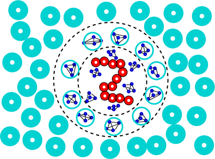
Figure 1: (Color online) A schematic plot of a solvated generic bead-spring polymer. The solvent is modeled on different levels of detail: solvent molecules within a certain radius from the polymer’s center of mass are represented with a high (atomistic) resolution while a lower mesoscopic resolution is used for the more distant solvent. The high resolution sphere moves with the polymer’s center of mass. The polymer beads are represented smaller than the solvent molecules for presentation convenience, for details see text.

Solvent molecules within a distance $r_{0}$ from the polymer’s center of mass are modeled with all ’atomistic’ details to properly describe the specific polymer-solvent interactions. For the description of the solvent farther away, where the high resolution is not required, we use a lower resolution. The solvent molecules then, depending on their distance to the polymer’s center of mass, automatically adapt their resolution on-the-fly.

The model solvent is a liquid of $n$ tetrahedral molecules as introduced in Refs. Praprotnik:2005:4 ; Praprotnik:2006 . The solvent molecules in the high resolution regime are composed of four equal atoms with mass $m_{0}$. Their size $\sigma$ is fixed via the repulsive Weeks-Chandler-Andersen potential

$$U_{rep}^{atom}(r_{i\alpha j\beta})=\\ \left\{\begin{array}[]{rc}4\varepsilon\bigl{[}\bigl{(}\frac{\sigma}{r_{i\alpha j\beta}}\bigr{)}^{12}-\bigl{(}\frac{\sigma}{r_{i\alpha j\beta}}\bigr{)}^{6}+\frac{1}{4}\bigr{]};&r_{i\alpha j\beta}\leq 2^{1/6}\sigma\\ 0;&r_{i\alpha j\beta}>2^{1/6}\sigma\end{array}\right.$$ (1)

with the cutoff at $2^{1/6}\sigma$. $\sigma$ and $\varepsilon$ are the standard Lennard Jones units for lengths and energy respectively. $r_{i\alpha j\beta}$ is the distance between the atom $i$ of the molecule $\alpha$ and the atom $j$ of the molecule $\beta$. The neighboring atoms in a given molecule $\alpha$ are connected by finite extensible nonlinear elastic (FENE) bonds

$$U_{bond}^{atom}(r_{i\alpha j\alpha})=\\ \left\{\begin{array}[]{rc}-\frac{1}{2}kR_{0}^{2}\ln\bigl{[}1-\bigl{(}\frac{r_{i\alpha j\alpha}}{R_{0}}\bigl{)}^{2}\bigr{]};&r_{i\alpha j\alpha}\leq R_{0}\\ \infty;&r_{i\alpha j\alpha}>R_{0}\end{array}\right.$$ (2)

with divergence length $R_{0}=1.5\sigma$ and stiffness $k=30\varepsilon/\sigma^{2}$, so that the average bond length is approximately $0.97\sigma$ for $k_{B}T=\varepsilon$, where $T$ is the temperature of the system and $k_{B}$ is Boltzmann’s constant. For the coarse-grained solvent model in the low resolution regime we use one-site spherical molecules interacting via an effective pair potentialPraprotnik:2006 , which was derived such that the statistical properties, i.e., the center of mass radial distribution function and pressure, of the high resolution liquid are accurately reproduced. This is also needed for the present study, since the motion of the high resolution sphere should not be linked to strong rearrangements in the liquid. The high and low resolution freely exchange molecules through a transition regime containing hybrid molecules (see figure 1), where the molecules with no extra equilibration adapt their resolution and change the number of DOFs accordinglyPraprotnik:2005:4 ; Praprotnik:2006 ; Praprotnik:2006:1 .

The polymer is modeled as a standard bead-spring polymer chainKremer:1990 . It contains $N$ monomers, which represent chemical repeat units, usually comprising several atoms. The interactions between monomers (beads) are defined using Eqs. (1) and (2) with the rescaled values $\sigma_{B}=1.8\sigma$, $R_{0_{B}}=R_{0}\sigma_{B}/\sigma=1.5\sigma_{B}$, and $k_{B}=k\sigma^{2}/\sigma_{B}^{2}=30\varepsilon/\sigma_{B}^{2}$, such that the size of the polymer bead $\sigma_{B}$ is approximately the same as the size of the solvent moleculePraprotnik:2006 . The average bond length between beads is rescaled accordingly. The bead mass is also increased $m_{B}=5m_{0}$ to make them behave more like Brownian particles. Standard Lorentz-Berthelot mixing rulesAllen:1987 are used for the interaction between monomers and the ’atoms’ of the solvent molecules.

III Numerical Scheme and Computational Details

To smoothly couple the regimes of high and low level of detail of the description of the solvent molecules, we apply the recently introduced AdResS schemePraprotnik:2005:4 . There the molecules can freely move between the regimes, they are in equilibrium with each other with no barrier in between. The transition is governed by a weighting function $w(r)\in[0,1]$ that interpolates the molecular interaction forces between the two regimes, and assigns the identity of the solvent molecule. We resort here to the weighting function defined in Ref. Praprotnik:2006 :

$$w(r)=\left\{\begin{array}[]{rc}1;&r_{0}>r\geq 0\\ 0;&r\geq r_{0}+d\\ \cos^{2}[\frac{\pi}{2d}(r-r_{0})];&r_{0}+d>r\geq r_{0}\end{array}\right.$$ (6)

where $r_{0}$ is the radius of the high resolution region and $d$ the interface region width, cf. 1. The radius $r_{0}$ must be chosen sufficiently large so that the whole polymer always stays within the high resolution solvent regime. $w(r)$ is defined in such a way that $w=1$ corresponds to the high resolution, $w=0$ to the low resolution, and values $0<w<1$ to the transition regime, respectively. This leads to intermolecular force acting between centers of mass of solvent molecules $\alpha$ and $\beta$:

$${\bf F}_{\alpha\beta}=w(|{\bf R}_{\alpha}-{\bf R}|)w(|{\bf R}_{\beta}-{\bf R}|){\bf F}_{\alpha\beta}^{ex}\\ +[1-w(|{\bf R}_{\alpha}-{\bf R}|)w(|{\bf R}_{\beta}-{\bf R}|)]{\bf F}_{\alpha\beta}^{cg}.$$ (7)

${\bf F}_{\alpha\beta}$ is the total intermolecular force acting between centers of mass of the solvent molecules $\alpha$ and $\beta$. ${\bf F}_{\alpha\beta}^{ex}$ is the sum of all pair ’atom’ interactions between explicit tetrahedral ’atoms’ of the solvent molecule $\alpha$ and explicit tetrahedral ’atoms’ of the solvent molecule $\beta$, ${\bf F}_{\alpha\beta}^{cg}$ is the effective pair force between the two solvent molecules, and ${\bf R}_{\alpha}$, ${\bf R}_{\beta}$, and ${\bf R}$ are the centers of mass of the molecules $\alpha$, $\beta$ and the polymer, respectively. Note that one has to interpolate the forces and not the interaction potentials in Eq. (7) if the Newton’s Third Law is to be satisfied Praprotnik:2006:1 . To suppress the unphysical density and pressure fluctuations emerging as artifacts of the scheme given in Eq. (7) within the transition zone we employ an interface pressure correctionPraprotnik:2006 . The latter involves a reparametrization of the effective potential in the system composed of exclusively hybrid molecules with $w=1/2$. Each time a solvent molecule crosses a boundary between the different regimes it gains or looses on-the-fly (depending on whether it leaves or enters the coarse-grained region) its equilibrated rotational and vibrational DOFs while retaining its linear momentumPraprotnik:2006:1 ; Praprotnik:2005 ; Praprotnik:2005:1 ; Praprotnik:2005:2 . This change in resolution requires to supply or remove ”latent heat” and thus must be employed together with a thermostat that couples locally to the particle motion Praprotnik:2005:4 ; Praprotnik:2006:1 . This is achieved by coupling the particle motion to the Dissipative Particle Dynamics (DPD) thermostatSoddemann:2003 . This bears the additional advantage of preserving momentum conservation and correct reproduction of hydrodynamics in our $nVT$ MD simulations. Because of the freely moving polymer chain and solvent molecules, the above scheme requires the center of the high resolution sphere to move with the polymer but slowly compared to the surrounding solvent molecules, so that they at the boundary between different regimes have enough time to adapt to the resolution change. The validity condition for our approach thus requires $D_{polymer}\ll D_{solvent}$, where $D_{polymer}$ and $D_{solvent}$ the corresponding diffusion constants. This condition is trivially fulfilled in polymeric solutions and thus also in our simulations (see the next section).

We conducted all MD simulations using the ESPResSo packageEspresso:2005 . We integrated Newtons equations of motion by a standard velocity Verlet algorithm with a time step $\Delta t=0.005\tau$ and coupled the motion of the particles to a DPD theromstatSoddemann:2003 with the temperature set to $T=\varepsilon/k_{B}$. The DPD friction constant $\zeta=0.5\tau^{-1}$, where $\tau=(\varepsilon/m_{0}\sigma^{2})^{-1/2}$, and the DPD cutoff radius was set equal to the cuttoff radius of the effective pair interaction between solvent molecules, i.e., $3.5\sigma$Praprotnik:2006 . The width of the transition regime is $2.5\sigma$Praprotnik:2006 . Periodic boundary conditions and the minimum image conventionAllen:1987 were employed. After equilibration, trajectories of $5000\tau$ were obtained, with configurations stored every $5\tau$. These production runs were performed with a $10^{9}\varepsilon/\sigma$ force capping to prevent possible force singularities that could emerge due to overlaps with the neighboring molecules when a given molecule enters the transition layer from the coarse-grained side Praprotnik:2005:4 . The temperature was calculated using the fractional analog of the equipartition theorem:

$$\left<K_{\alpha}\right>=\frac{\alpha k_{B}T}{2},$$ (8)

where $\left<K_{\alpha}\right>$ is the average kinetic energy per fractional quadratic DOF with the weight $w(r)=\alpha$Praprotnik:2006:1 . Via Eq. (8) the temperature is also rigorously defined in the transition regime in which the vibrational and rotational DOFs are partially ’switched on/off’. The molecular number density of the solvent is $\rho=0.175/\sigma^{3}$, which corresponds to a typical high density Lennard-Jones liquidPraprotnik:2006 . We considered three different system sizes with corresponding cubic box sizes: $L=25.0\sigma,30.6\sigma,34.2\sigma$. The reduced Lennard-Jones unitsAllen:1987 are used in the remainder of the paper.

IV Results and Discussion

To validate the AdResS approach for the present polymer solvent system, we carried out the analysis of the structural and dynamic properties of a polymer chain in the hybrid multiscale solvent compared to the corresponding fully explicit system where all solvent molecules are modeled with a high level of detail, i.e., as a tetrahedral molecules.

IV.1 Statics of the Polymer Chain and Solvent

First, we focus on the explicit (ex) systems where the solvent is modeled with the high resolution all over the simulation box. These results are considered as the reference to check how well AdResS produces the same physics as the all-atom MD simulation. The reference average thermodynamic properties of the corresponding ex systems (polymer+explicitely resolved solvent) are listed in table 1.

$N$	$10$	$20$	$30$
$L$	$25.0$	$30.6$	$34.2$
$<p>$	$2.01\pm 0.04$	$2.01\pm 0.03$	$2.02\pm 0.01$
$<T>$	$1.0\pm 0.01$	$1.0\pm 0.01$	$1.0\pm 0.01$
$<T_{polymer}>$	$1.0\pm 0.5$	$1.0\pm 0.3$	$1.0\pm 0.2$
$<T_{solvent}>$	$1.0\pm 0.01$	$1.0\pm 0.01$	$1.0\pm 0.01$

Table 1: Thermodynamic properties of the fully explicit systems (ex) of different chain lengths $N$ and box sizes $L$: average total pressure $\left<p\right>$, average total temperature of the system $\left<T\right>$, average temperature of the polymer $\left<T_{polymer}\right>$, and average temperature of the solvent $\left<T_{solvent}\right>$.

The static properties of the solvent are characterized by the solvent radial center of mass distribution (RDF) function depicted in figures 2 (a). This distribution function is within the thickness of the lines the same for all systems studied, including the hybrid ones. This is to be expected from our previous studies and the fact, that the polymer fraction of volume is very small compared to that of the solvent.

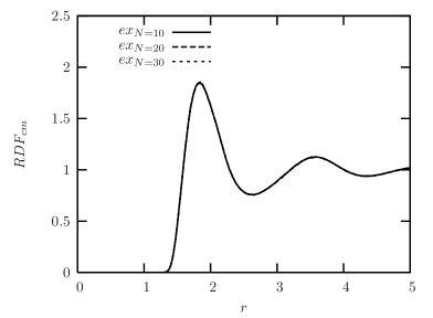
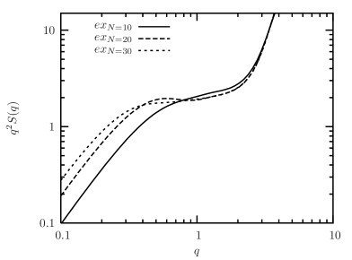
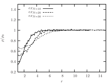
Figure 2: (a) The solvent center of mass RDF for three different polymer lengths (N=10,20,30), (b) the static structure factor of the polymer in the Kratky representation, and (c) the solvent density around the center of mass of the chains, which illustrates the so called correlation hole.

The statistical properties of polymers are conveniently described by a number of quantities, namely the radius of gyration

$$\left<R_{G}^{2}\right>=\frac{1}{N}\sum_{i}\left<({\bf r}_{i}-{\bf R})^{2}\right>,$$ (9)

where ${\bf r}_{i}$ is the position vector of the $i$th monomer and ${\bf R}=N^{-1}\sum_{i}{\bf r}_{i}$ is the polymer’s center of mass, the end-to-end distance

$$\left<R_{E}^{2}\right>=\left<({\bf r}_{N}-{\bf r}_{1})^{2}\right>,$$ (10)

and the hydrodynamic radius

$$\left<\frac{1}{R_{H}}\right>=\frac{1}{N^{2}}\sum_{i\neq j}\left<\frac{1}{r_{ij}}\right>,$$ (11)

where $r_{ij}=|{\bf r}_{i}-{\bf r}_{j}|$Praprotnik:2006:3 .

$\left<R_{G}^{2}\right>$ and $\left<R_{E}^{2}\right>$ scale as

$$\left<R_{G}^{2}\right>\propto\left<R_{E}^{2}\right>\propto N^{2\nu}$$ (12)

with the number of monomers $N$ where $\nu=0.5$ in $\theta$ solvent and $\nu\approx 0.588$ in good solvent conditionsGennes:1979 ; Doi:1986 ; Sokal:1995 with rather small finite size corrections, while the hydrodynamic radius is known to show significant deviations from asymptotic behavior up to very long chainsDunweg:1993 .

The single-chain static structure factor $S(q)$

$$S(q)=\frac{1}{N}\left<\sum_{ij}\exp(i{\bf q}\cdot({\bf r}_{i}-{\bf r}_{j}))\right>$$ (13)

probes the self similar structure within the scaling regime and thus provides an accurate way to determine $\nu$. $S(q)$ scales as

$$S(q)\propto q^{-1/\nu}\rightarrow q^{2}S(q)\propto q^{2-1/\nu}$$ (14)

in the regime $R_{G}^{-1}\ll q\ll b^{-1}$, where $b$ is the typical bond length. By fitting a power law to the computed $q^{2}S(q)$ plotted in figure 2 (b) we obtained the values for $\nu$ reported in table 2. Table 2 summarizes the values of all quantities defined above, which characterize the static properties of the polymer chain. The calculations were performed for $N=10,20,30$.

$N$	$10$	$20$	$30$
$L$	$25.0$	$30.6$	$34.2$
$\left<\Delta r_{max}\right>$	$4.2\pm 0.8$	$5.7\pm 1.0$	$8.1\pm 1.4$
$R_{G}=\left<R_{G}^{2}\right>^{1/2}$	$2.7\pm 0.5$	$3.8\pm 0.6$	$5.0\pm 0.8$
$R_{E}=\left<R_{E}^{2}\right>^{1/2}$	$6.7\pm 2.0$	$8.6\pm 3$	$12\pm 3$
$R_{H}=\left<R_{H}^{-1}\right>^{-1}$	$3.3\pm 0.3$	$4.0\pm 0.3$	$4.7\pm 0.4$
$\nu$	$0.63$	$0.54$	$0.57$
$2/z$	$0.59$	$0.71$	$0.67$
$\tau=R_{G}^{2}/(6D)$	$152$	$481$	$1390$

Table 2: Summary of some polymer (embedded in the explicitely resolved ex solvent) properties: number of polymer beads $N$, size of the simulation box $L$, average maximal distance of a monomer from the polymer’s center of mass $\left<\Delta r_{max}\right>$, radius of gyration $R_{G}$, end-to-end distance $R_{E}$, hydrodynamic radius $R_{H}$, the static exponent $\nu$, the exponent $2/z$, where $z$ is the dynamic exponent, and the longest relaxation time $\tau$ calculated using data from table 6. The error bar for the exponents $\nu$ and $2/z$ is roughly $10\%$.

Another property, which directly reveals the fractal structure of the chains is the correlation hole, which is shown in figure 2 (c). It directly shows, to which distance from the center of mass of the chains, the solvent density is perturbed by the chain beads. For the later application of the hybrid scheme it is important to define the explicit solvent regime large enough in order to cover the correlation hole completely.

The values of $\nu$ actually differ slightly from the asymptotical value for the good solvent due to the finite chain lengths. Nevertheless, the agreement improves with the increasing $N$, as expected.

Let us now turn our attention to the hybrid solvent studied by MD simulation using AdResS.

To assure that the polymer is surrounded only by the explicitely resolved molecules, we determine first the maximal monomer distance from the polymer’s center of mass, $\Delta r_{max}$, as shown in figure 3 for all chain lengths studied.

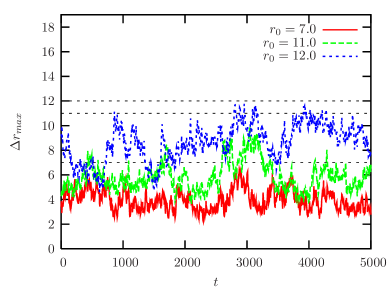
Figure 3: (Color online) Time evolution of the maximal monomer distance from the polymer’s center of mass, $\Delta r_{max}$, for polymers with $N=10$ beads and the radius of the high resolution regime $r_{0}=7.0$ (red line), $N=20$ and $r_{0}=11.0$ (green line), and $N=30$ and $r_{0}=12.0$ (blue line).

As shown $\Delta r_{max}$ always stays within the high resolution regime.

Because for $N=30$ $\Delta r_{max}$ gets rather close to $r_{0}$, we checked the static polymer properties for that case again. In figure 4 we compare the all explicit simulation to the two hybrid simulation schemes (with (ex-cg_ic) and without (ex-cg) the pressure correctionPraprotnik:2006 in the transition regime) for the chain form factor and the correlation hole. The agreement is excellent, showing that the proposed scheme should at least be capable of properly reproducing the conformational statistics of the embedded polymer in solution.

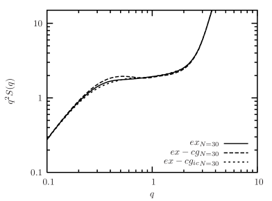
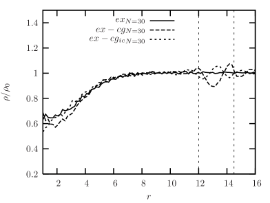
Figure 4: (a) The the static structure factor of the polymer with $N=30$ in the Kratky representation for all three cases studied: the fully explicite, the AdResS scheme with and without the interface pressure correction. (b) The correlation hole for the same systems as in (a).

This is first checked by comparing the average thermodynamic properties as given in table 3 for the hybrid ex-cg and ex-cg_ic systems (polymer+hybrid solvent). While the temperatures are identical the pressure correction in the interface layer reduces the pressure slightly, so that the hybrid system now also there agrees quite well with the all explicit simulation.

$N$	$10$	$20$	$30$
$L$	$25.0$	$30.6$	$34.2$
$<p>_{ex-cg}$	$2.03\pm 0.02$	$2.04\pm 0.01$	$2.04\pm 0.03$
$<p>_{ex-cg_{ic}}$	$2.01\pm 0.01$	$2.01\pm 0.01$	$2.01\pm 0.01$
$<T>$	$1.0\pm 0.02$	$1.0\pm 0.01$	$1.0\pm 0.01$
$<T_{polymer}>$	$1.0\pm 0.5$	$1.0\pm 0.3$	$1.0\pm 0.2$
$<T_{solvent}>$	$1.0\pm 0.02$	$1.0\pm 0.01$	$1.0\pm 0.01$

Table 3: Thermodynamic properties of systems with the polymer solvated in the hybrid ex-cg solvent and the hybrid ex-cg_ic solvent: average total pressure $\left<p\right>$, average total temperature of the system $\left<T\right>$, average temperature of the polymer $\left<T_{polymer}\right>$, and average temperature of the solvent $\left<T_{solvent}\right>$. For the temperatures the results cannot be distinguished.

The agreement with the reference values from table 1 is very good. This is in line with the general static properties of the polymers, which are given in 4 and 5, and compare very well to the data from table 2.

$N$	$10$	$20$	$30$
$L$	$25.0$	$30.6$	$34.2$
$r_{0}$	$7.0$	$11.0$	$12.0$
$\left<\Delta r_{max}\right>$	$4.2\pm 0.8$	$6.6\pm 1.2$	$7.7\pm 1.3$
$R_{G}=\left<R_{G}^{2}\right>^{1/2}$	$2.7\pm 0.4$	$4.0\pm 0.6$	$4.6\pm 0.7$
$R_{E}=\left<R_{E}^{2}\right>^{1/2}$	$6.7\pm 2.0$	$10.4\pm 2.8$	$10.8\pm 2.5$
$R_{H}=\left<R_{H}^{-1}\right>^{-1}$	$3.3\pm 0.3$	$4.0\pm 0.3$	$4.5\pm 0.4$
$\nu$	$0.63$	$0.58$	$0.54$
$2/z$	$0.56$	$0.69$	$0.62$
$\tau=R_{G}^{2}/(6D)$	$122$	$381$	$882$

Table 4: Summary of some polymer (embedded in the hybrid ex-cg solvent) properties: number of polymer beads $N$, size of the simulation box $L$, radius of the high resolution regime $r_{0}$, average maximal distance of a monomer from the polymer’s center of mass $\left<\Delta r_{max}\right>$, radius of gyration $R_{G}$, end-to-end distance $R_{E}$, hydrodynamic radius $R_{H}$, the static exponent $\nu$, the exponent $2/z$, where $z$ is the dynamic exponent, and the longest relaxation time $\tau$ calculated using data from table 6. The error bar for the exponents $\nu$ and $2/z$ is roughly $10\%$.

$N$	$10$	$20$	$30$
$L$	$25.0$	$30.6$	$34.2$
$r_{0}$	$7.0$	$11.0$	$12.0$
$<\Delta r_{max}>$	$4.0\pm 0.8$	$5.9\pm 1.2$	$8.6\pm 1.5$
$R_{G}=\left<R_{G}^{2}\right>^{1/2}$	$2.7\pm 0.5$	$3.9\pm 0.7$	$5.2\pm 0.8$
$R_{E}=\left<R_{E}^{2}\right>^{1/2}$	$6.6\pm 2.1$	$9.4\pm 3.0$	$13.3\pm 3.3$
$R_{H}=\left<R_{H}^{-1}\right>^{-1}$	$3.2\pm 0.3$	$4.0\pm 0.4$	$4.8\pm 0.4$
$\nu$	$0.59$	$0.55$	$0.57$
$2/z$	$0.69$	$0.71$	$0.77$
$\tau=R_{G}^{2}/(6D)$	$152$	$362$	$1127$

Table 5: Same data as in table 4, but now for the hybrid ex-cg_ic, where interface pressure correction is applied.

From the presented results we can conclude that AdResS faithfully reproduces the reference statics obtained from the simulations with a polymer embedded in the explicitely resolved solvent.

IV.2 Dynamics of the Polymer Chain and Solvent

While the conformational properties of the polymer in solution are well understood and properly described by the adaptive resolution approach, the situation for the dynamics is much less clear. By changing the degrees of freedom not only the structure but also the dynamical properties are altered, however in a way which is less understood. It is also not a priori clear, whether an approach, which produces a precise coarse graining for structural properties, does this for dynamical properties as well. In a recent study of small additive molecules to a polymer melt it was shown, that while the length scaling is identical, the time scaling can be differentHarmandaris:2007 . In the present situation the influence of the transition regime poses additional difficulties.

In order to determine the dynamical properties of the solvent and solute we calculated the respective diffusion coefficients. The diffusion coefficient of a species is computed from the center of mass displacements using the Einstein relation

$$D=\frac{1}{6}\lim_{t\rightarrow\infty}\frac{\langle|{\bf R}_{i}(t)-{\bf R}_{i}(0)|^{2}\rangle}{t}=\frac{1}{6}\lim_{t\rightarrow\infty}\frac{\langle\Delta R^{2}\rangle}{t},$$ (15)

where ${\bf R}_{i}(t)$ is the center-of-mass position of the molecule $i$ (which can be either a solvent or a solute molecule) at time $t$ and averaging is performed over all choices of time origin and, in the case of solvent, over all solvent molecules.

Figure 5 shows this for the solvent molecules’ centers of mass as a function of time for the different systems indicated. All the curves in figure 5, except the one for the coarse-grained solvent coincide. Thus the effect of the polymer on the diffusivity of the solvent molecules is negligible. In other words, the dilution is strong enough that the polymer effect on the solvent dynamics is very small. The coarse grained solvent molecules however move faster than the explicit ones. This is a consequence of the reduced number of DOFs causing a time scale difference in the dynamics of the coarse-grained systemPraprotnik:2005:4 ; Praprotnik:2006 . While this can be very advantageous in some cases, one can also adjust $D$ by an increased background friction in the DPD thermostatKremer:1990 ; Izvekov:2006 .

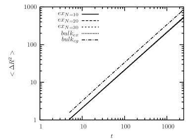
Figure 5: Log-log plot of the time dependence of the mean square displacement of the solvent molecule’s center of mass in the. time interval [0,5000]: explicitely resolved (bulk_ex) and coarse-grained (bulk_cg) solvents without solvated polymer and the explicitely resolved solvent for the systems with three different lengths of the solvated polymer (N=10,20,30).

The diffusion coefficient $D$ of the solvent was obtained by fitting a linear function to the curves depicted in figure 5 (a) and the obtained values are $D_{bulk_{ex}}=0.036$ and $D_{bulk_{cg}}=0.057$ for the explicit and coarse-grained solvent, respectively. The question to ask here is, to what extend does this have any influence on the dynamics of the embedded polymer.

Within the Zimm modelDoi:1986 for polymer chain dynamics, which is known to describe the scaling of the dynamics in dilute solutions of polymers rather well and which takes into account the hydrodynamic interactions, the polymer diffusion coefficient scales as

$$D\propto N^{-\nu}\propto R_{H}^{-1}\propto R_{G}^{-1}.$$ (16)

The longest relaxation time $\tau=R_{G}^{2}/(6D)$, i.e., the Zimm time $\tau_{Z}\propto R_{G}^{3}=R_{G}^{z}$, is the time the chain needs to move its own size. $z=3$ is the dynamic exponent. Note that the motion of inner monomers within the appropriate scaling regime should be independent of $N$. For the mean square displacements of the monomers a scaling analysis immediately yields for the mean square displacement of a monomer $i$,

$$\langle\Delta r^{2}\rangle=\langle({\bf r}_{i}(t)-{\bf r}_{i}(0))^{2}\rangle\propto t^{2/z}=t^{2/3},$$ (17)

for distances significantly larger than the bond length and smaller than $\langle R^{2}\rangle$, i.e., times smaller than $\tau_{Z}$. For the center of mass of the chains a diffusive behavior for the mean square displacement $\langle\Delta R^{2}(t)\rangle$ is always observed. Although the chains are relatively short, at least for $N=30$ one expects a behavior relatively close to the above mentioned idealized schemeDunweg:1993 . Figure 6 shows $\langle\Delta r^{2}(t)\rangle$ and $\langle\Delta R^{2}(t)\rangle$ for polymer chains with $N=10,20,30$ embedded in the different solvent scenarios studied.

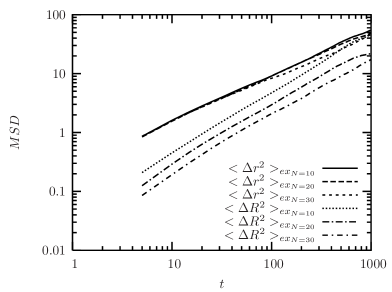
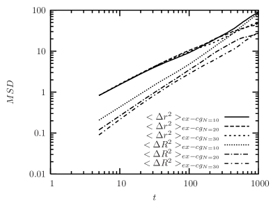
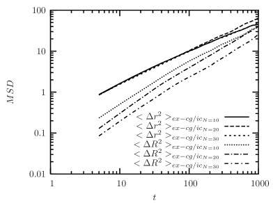
Figure 6: Log-log plot of the time dependence of the mean square displacement of a single monomer (considered are only monomers near the chain’s center of mass) for polymers and their centers of mass with $N=10,20,30$ solvated in the ex solvent (a), the hybrid ex-cg solvent (b) and the ex-cg_ic solvent (c) as indicated.

In all cases the observed exponents for $\langle\Delta r^{2}(t)\rangle$ and $\langle\Delta R^{2}(t)\rangle$ are close to $0.7\pm 0.05$ and $1\pm 0.05$ respectively. Also the amplitudes of the displacements of the inner beads are almost the same for all chain lengths studied. This is in good agreement with earlier studies on different generic polymer models in a explicit solvent as well as studies of chains in a hybrid lattice Boltzmann solventDunweg:1993 ; Ahlrichs:1999 . This is to be expected since we preserve the hydrodynamic interactions by employing the DPD thermostat in our simulations. This suggests that our hybrid scheme is also applicable to study dynamic properties of a polymer in a solution. Small deviations however occur in the diffusion constant itself. The diffusion constants for the polymers with $N=10,20,30$ in the hybrid ex-cg and ex-cg_ic solvents were obtained by fitting the straight curve to the polymer’s center of mass mean square displacement presented in figure 6. The fit yields data listed in table 6. The corresponding static and dynamic exponents and the longest relaxation times are given in tables 4 and 5.

$N$	$10$	$20$	$30$
D(ex)	$0.008$	$0.005$	$0.003$
D(ex-cg)	$0.009$	$0.006$	$0.0045$
D(ex-cgic)	$0.0085$	$0.006$	$0.0035$

Table 6: Diffusion constant of the polymer chain embedded in three different solvents: explicitely resolved ex, hybrid ex-cg, and hybrid ex-cg_ic. Though the statistics of the data is rather poor we can estimate the error bar roughly to $10-15\%$. For comparison, the diffusion coefficients of the explicit and coarse-grained solvents are $D_{bulk_{ex}}=0.036$ and $D_{bulk_{cg}}=0.057$, respectively with an effect of the polymers too small to determine here. Hence $D_{polymer}\ll D_{solvent}$.

While the ratio of the diffusion constants for different chain lengths roughly follow the expected scaling, even though it cannot hold precisely due to the different box sizes, we here observe a tendency to a weakly accelerated diffusion in the hybrid regime. This is most evident for the hybrid ex-cg case. Two different aspects might play a role here. First the viscosity in the coarse grained outer regime is smaller, which must have an effect on the diffusion. Second, the small pressure and density fluctuations in the transition regime might contribute to the effect as well.

Although this is only a very first and incomplete test, it shows that within the AdResS scheme essential aspects of the dynamical properties of the embedded polymer chain are reasonably well reproduced.

V Summary and Outlook

In this paper we presented a hybrid multiscale MD simulation of a generic macromolecule in a solvent using the recently proposed AdResS method. The solvent surrounding the macromolecule is represented with a sufficiently high level of detail so that the specific interactions between the solvent and the solute are correctly taken into account. The solvent farther away from the macromolecule, where the high resolution is not needed, is represented on a coarse-grained level. The high and low resolution regimes freely exchange solvent molecules, which change their resolution accordingly. To correctly simulate momentum transport through the solvent, we use the DPD thermostat. The simulation results show that AdResS accurately reproduces the thermodynamic and structural properties of the system. The presented methodology is an extension of AdResS to simulations of a solvation cavity, and represents a first step towards the treatment of more realistic systems such as biomacromolecules embedded in water. Work along these lines is already under wayPraprotnik:2006:2 .

References

- (1) G. Careri, in Hydration Processes in Biology: Theoretical and Experimental Approaches, edited by M. C. Bellisient-Funel, pages 143–155, IOS, Amsterdam, 1999.
- (2) P. Das, S. Matysiak, and C. Clementi, Proc. Natl. Acad. Sci. U. S. A. 102, 10141 (2005).
- (3) E. Villa, A. Balaeff, and K. Schulten, Proc. Natl. Acad. Sci. U.S.A. 102, 6783 (2005).
- (4) H. Rafii-Tabar, L. Hua, and M. Cross, J. Phys.: Condens. Matter 10, 2375 (1998).
- (5) J. Q. Broughton, F. F. Abraham, N. Bernstein, and E. Kaxiras, Phys. Rev. B 60, 2391 (1999).
- (6) P. Ahlrichs and B. Dünweg, J. Chem. Phys. 111, 8225 (1999).
- (7) A. Malevanets and R. Kapral, J. Chem. Phys. 112, 7260 (2000).
- (8) G. Csanyi, T. Albaret, M. C. Payne, and A. DeVita, Phys. Rev. Lett. 93, 175503 (2004).
- (9) C. F. Abrams, J. Chem. Phys. 123, 234101 (2005).
- (10) M. Neri, C. Anselmi, M. Cascella, A. Maritan, and P. Carloni, Phys. Rev. Lett. 95, 218102 (2005).
- (11) G. D. Fabritiis, R. Delgado-Buscalioni, and P. V. Coveney, Phys. Rev. Lett. 97, 134501 (2006).
- (12) M. Praprotnik, L. Delle Site, and K. Kremer, J. Chem. Phys. 123, 224106 (2005).
- (13) M. Praprotnik, L. Delle Site, and K. Kremer, Phys. Rev. E 73, 066701 (2006).
- (14) M. Praprotnik, K. Kremer, and L. Delle Site, Phys. Rev. E 75, 017701 (2007).
- (15) M. Praprotnik, L. Delle Site, K. Kremer, S. Matysiak, and C. Clementi, cond-mat/0611544 (2006).
- (16) K. Kremer and G. S. Grest, J. Chem. Phys. 92, 5057 (1990).
- (17) M. P. Allen and D. J. Tildesley, Computer Simulation of Liquids, Clarendon Press, Oxford, 1987.
- (18) D. Janežič, M. Praprotnik, and F. Merzel, J. Chem. Phys. 122, 174101 (2005).
- (19) M. Praprotnik and D. Janežič, J. Chem. Phys. 122, 174102 (2005).
- (20) M. Praprotnik and D. Janežič, J. Chem. Phys. 122, 174103 (2005).
- (21) T. Soddemann, B. Dünweg, and K. Kremer, Phys. Rev. E 68, 046702 (2003).
- (22) http://www.espresso.mpg.de.
- (23) Note that the definition of given in Eq. (11) is only correct for an infinite simulation box. For a finite box we have to also consider the hydrodynamic interactions with the periodic images. The value of in such a way corrected deviates from the value obtained using the formula (11)Dunweg:1993 ; Ahlrichs:1999 . However, since our aim in the present work is only to compare the properties of the polymer chain from the hybrid simulation with the corresponding ones from the all-atom simulation we here do not take the finite size correction into account and use the formula (11) for the definition of .
- (24) P.-G. de Gennes, Scaling Concept in Polymer Physics, Cornell University, Ithaca, 1979.
- (25) M. Doi and S. F. Edwards, The Theory of Polymer Dynamics, Clarendon, Oxford, 1986.
- (26) A. D. Sokal, in Monte Carlo and Molecular Dynamics Simulation in Polymer Science, edited by K. Binder, chapter 2, Clarendon, Oxford, 1995.
- (27) B. Dünweg and K. Kremer, J. Chem. Phys. 99, 6983 (1993).
- (28) V. A. Harmandaris, N. P. Adhikari, N. F. A. van der Vegt, K. Kremer, R. Voelkel, H. Weiss, and CheeChin Liew, Macromolecules, submitted.
- (29) S. Izvekov and G. A. Voth, J. Chem. Phys. 125, 151101 (2006).