Local spin density in two-dimensional electron gas with hexagonal boundary

Abstract

The intrinsic spin-Hall effect in hexagon-shaped samples is investigated. To take into account the spin-orbit couplings and to fit the hexagon edges, we derive the triangular version of the tight-binding model for the linear Rashba [Sov. Phys. Solid State 2, 1109 (1960)] and Dresselhaus [Phys. Rev. 100, 580 (1955)] [001] Hamiltonians, which allow direct application of the Landauer-Keldysh non-equilibrium Green function formalism to calculating the local spin density within the hexagonal sample. Focusing on the out-of-plane component of spin, we obtain the geometry-dependent spin-Hall accumulation patterns, which are sensitive to not only the sample size, the spin-orbit coupling strength, the bias strength, but also the lead configurations. Contrary to the rectangular samples, the accumulation pattern can be very different in our hexagonal samples. Our present work provides a fundamental description of the geometry effect on the intrinsic spin-Hall effect, taking the hexagon as the specific case. Moreover, broken spin-Hall symmetry due to the coexistence of the Rashba and Dresselhaus couplings is also discussed. Upon exchanging the two coupling strengths, the accumulation pattern is reversed, confirming the earlier predicted sign change in spin-Hall conductivity.

I Introduction

Spintronics, a science investigating the mechanism of electron spins, has stimulated general theoretical interests in and attempts of industrial application on how to control electron spins.App1 ; App2 By coupling the electron spin to the charge degrees of freedom, the spin-orbit (SO) interaction makes manipulating spin electrically possible. In particular, the spin-Hall effect (SHE), originating from such interaction, has attracted lots of researchers’ attention since it induces a pure transverse spin current simply as a response to the longitudinal charge current.

According to the sources of SO interaction, two types of the SHE can be identified: (i) extrinsic SHEDyakonov ; Hirch ; Zhang ; Extrinc with SO coupling being sourced by the external impurities, and (ii) intrinsic SHE (ISHE) with inherent SO coupling in the system. In both effects, the SO interaction subjects the spin-up ($+z$) and spin-down ($-z$) electrons respectively to opposite forces perpendicular to their transport direction. As a result, up-spin piles up on one side while down-spin on the other of the sample (in $x$-$y$ plane), forming the so-called spin-Hall accumulation (SHA). Inspired by the recent breakthrough in experiments,Y.K.Kato these two effects are intensively under investigation in bulk semiconductors,Th1 ; Th2 ; Th3 ; Th4 ; Th5 ; Th6 ; Th7 two-dimensional semiconductor heterostructures,Th8 ; Th9 ; Th10 ; Th11 ; Sinova1 ; Sinova2 ; Nikolic ; Nikolic2 ; Finite1 ; Finite2 ; Finite3 ; SOforce as well as the laterally confined quantum wires.QW1 ; QW2 Moreover, due to the stronger magnitude of spin current in the intrinsic case than in the extrinsic case (several orders greater), the ISHE has attracted intensive interests in theoretical study since the pioneering proposals.Th1 ; Sinova1 Nevertheless, most investigations focus on the rectangular geometry. The affection of the boundary in other shapes is rarely discussed. Characterizing the SHE in finite system,Nikolic ; Nikolic2 ; Finite1 ; Finite2 ; Finite3 ; SOforce this boundary degree of freedom as well as the varieties in bias configurations offer alternative ways for manipulating spin, and thus can further generate other applications.

In this paper we study the geometry effect by considering a clean two-dimensional electron gas (2DEG) with hexagonal shape, which gives us more degrees of freedom in contacting the sample. Inside the 2DEG, two kinds of well-known and commonly referred SO couplings are considered: the Rashba SO (RSO) and the Dresselhaus SO (DSO) couplings. The former is related to the inversion asymmetry of the structureRashba with its coupling strength adjustable via the gate voltage;Nitta ; Das2 the latter is caused by bulk inversion asymmetryDresselhaus ; Lommer with coupling strength depending on the material.Dyakonov2 ; Bastard Employing the Landauer-Keldysh (LK) Green function method in real space,Nikolic ; Nikolic2 ; Dattabook we analyze the $z$ component SHA pattern inside the hexagon-shaped Landauer setup with two to six terminals, each of which may be contacted by a semi-infinite ideal lead. Electrochemical potential differences between these leads induce longitudinal charge current among terminals. Contrary to the SHE in rectangular samples with two head-to-tail leads, the SHA patterns in our hexagonal 2DEG preserve the fundamental spin-Hall symmetry: the spins accumulate symmetrically (same magnitude) but oppositely (different sign) about the charge current flow direction, which is in general not straight in our hexagonal samples. Moreover, presented accumulation patterns are found to depend on (i) SO interaction strength, (ii) bias strength, (iii) sample size, (iv) lead configuration, and (v) SO interaction type, among which we put more emphasis on the last three. For factors (iii) and (v), a SHA reversal effect (SHARE) is identified and discussed in detail. In particular, upon interchanging the RSO and DSO coupling strengths for factor (v) the whole SHA pattern is reversed, confirming the sign change in the spin-Hall conductivity as previously predicted in Ref. Sinova2, . As for factor (iv), the accumulation pattern in certain lead configuration may be very different from those in rectangular samples.

This paper is organized as follows. In order to apply the real space tight-binding Hamiltonian in the LK formalism and fit the hexagon edges with appropriate discrete spatial points, we derive the triangular lattice version for the linear Rashba and Dresselhaus tight-binding model in Sec. II. This version also enables further study of the geometry effect on the SHE with other shapes such as triangle, trapezoid, diamond, parallelogram, arrow, etc. Section III gives a brief review on the LK formalism. Numerical results for SHA patterns based on the techniques introduced in Sec. II and Sec. III in various hexagonal samples will be reported and discussed in Sec. IV, in the zero temperature limit. We finally conclude in Sec. V.

II Tight-binding (finite differences) model in triangular lattice with RSO and DSO couplings

In this section, we approach the original Hamiltonian by discretizing the continuous space into lattice-like points with the finite difference method. The following results are thus reliable as the electron wave length is much longer than the distance between nearest points. This method exactly treats the Hamiltonian when the realistic lattice points match the ones in finite differences, and it is also a very general approach for any lattice structures. With the constructed triangular lattice, we intend to answer the essential questions on how the sample boundary, which is basically controllable in today’s technology, affects the spin accumulation.

Consider a hexagon-shaped 2DEG (set in the $x$-$y$ plane and grown along [001]) described by the Hamiltonian

$$\mathcal{H}=\mathcal{H}^{K}+\mathcal{H}^{R}+\mathcal{H}^{D},$$ (1)

where $\mathcal{H}^{K}=p^{2}/2m^{\star}$ (with $m^{\star}$ being the electron effective mass) is the kinetic energy, and

$$\mathcal{H}^{R} =\frac{\alpha}{\hbar}\left(p_{y}\sigma_{x}-p_{x}\sigma_{y}\right)$$ (2)

$$\mathcal{H}^{D} =\frac{\beta}{\hbar}\left(p_{x}\sigma_{x}-p_{y}\sigma_{y}\right)$$ (3)

denote the RSO and DSO Hamiltonians with coupling strengths $\alpha$ and $\beta$, respectively. Here $p_{x}$ and $p_{y}$ are the two independent contributions to the two-dimensional momentum operator: $\vec{p}=\left(p_{x},p_{y}\right)$, and the Pauli matrices $\vec{\sigma}=\left(\sigma_{x},\sigma_{y},\sigma_{z}\right)$ are used. To describe the system in real space, one can apply the tight-binding method to extract $\mathcal{H}$ in the real space lattice basis. However, to fit the hexagonal boundary, one has to discretize the space in triangular lattice structure, as shown in Fig. 1, where the lattice points are labeled as $0,1,\cdots,6$, while $A,B,\cdots,G$ are auxiliary points.

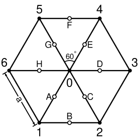
Figure 1: Schematic of the triangular lattice structure. On each lattice point, the electron has six nearest neighbors to hop.

Using the finite difference methodDattabook and labeling the wave function at position $\mathbf{r}$ as $\psi_{\mathbf{r}},$ the general expressions for first and second derivatives are approximated by

$$\left.\frac{\delta\mathbf{r}}{\delta r}\cdot\frac{d}{d\mathbf{r}}\psi_{{}_{\mathbf{r}}}\right|_{\mathbf{r}=\mathbf{\bar{r}}} =\frac{\left(\psi_{\mathbf{r}_{1}}-\psi_{\mathbf{r}_{2}}\right)}{\delta r},$$ (4)

$$\left.\left(\frac{\delta\mathbf{r}}{\delta r}\cdot\frac{d}{d\mathbf{r}}\right)^{2}\psi_{{}_{\mathbf{r}}}\right|_{\mathbf{r}=\mathbf{\bar{r}}} =\frac{\left(\psi_{\mathbf{r}_{1}}+\psi_{\mathbf{r}_{2}}-2\psi_{\mathbf{\bar{r}}}\right)}{\left(\delta r/2\right)^{2}},$$ (5)

with $\mathbf{\bar{r}\equiv}\left(\mathbf{r}_{1}+\mathbf{r}_{2}\right)/2$ and $\delta\mathbf{r\equiv r}_{1}-\mathbf{r}_{2}$. Thus the operation of these momentum operators can be expressed as

$$p_{x}\psi_{0} =\frac{-i\hbar}{a}\left(\psi_{H}-\psi_{D}\right)$$ (6a)

$$p_{y}\psi_{0} =\frac{-i\hbar}{\sqrt{3}a}\left(\psi_{F}-\psi_{B}\right),$$ (6b)

with $$a \overline{HD} \overline{FB} \mathcal{H} 0 \psi_{0} \psi_{1},\psi_{2},\cdots,\psi_{6}$$ being the lattice constant. Note the different denominators in Eqs. (6a) and (6b) due to the different distances between and . In order to construct the matrix representation of the Hamiltonian in the real space triangular lattice basis, our goal is to express the operation of on the wave function at point : , in terms of those on its nearest neighbors: .

Starting with the kinetic energy term, we take advantage of the isotropy of $\mathcal{H}^{K},$ which implies that the six directions (from site 0 to $1,2,\cdots,6$) in $\mathcal{H}^{K}$ should take the same form. From Eq. (4), we therefore have two additional momentum operators $p_{1}$ along $\overline{EA}$ and $p_{2}$ along $\overline{GC}$ with their operations on $\psi_{0}$ given by

$$p_{1}\psi_{0} =\frac{-i\hbar}{a}\left(\psi_{E}-\psi_{A}\right)$$ (7a)

$$p_{2}\psi_{0} =\frac{-i\hbar}{a}\left(\psi_{G}-\psi_{C}\right).$$ (7b)

Combining the three equal contributions from $$p_{x}, p_{1}, p_{2} t_{0}\equiv\hbar^{2}/2m^{\star}a^{2}$$ and [by using Eqs. (6a), (7a), and (7b)] and defining the hopping energy , straightforward substitution and rearrangement give

$$\frac{p_{1}^{2}+p_{2}^{2}+p_{x}^{2}}{2m^{\star}}\psi_{0}$$

$$=-t_{0}\left[\left(\psi_{1}+\psi_{4}-2\psi_{0}\right)+\left(\psi_{2}+\psi_{5}-2\psi_{0}\right)\right.$$

$$\left.+\left(\psi_{3}+\psi_{6}-2\psi_{0}\right)\right]$$ (8)

$$=-t_{0}\left[\left(\psi_{2}+\psi_{4}-2\psi_{D}\right)+\left(\psi_{1}+\psi_{5}-2\psi_{H}\right)\right.$$

$$\left.+\left(\psi_{3}+\psi_{6}-2\psi_{0}\right)\right]-2t_{0}\left(\psi_{D}+\psi_{H}-2\psi_{0}\right).$$

From the above equation, together with Eq. (5), we deduce $\left[\left(p_{1}^{2}+p_{2}^{2}+p_{x}^{2}\right)/2m^{\star}\right]\psi_{0}=\left(3/2\right)\left[\left(p_{x}^{2}+p_{y}^{2}\right)/2m^{\star}\right]\psi_{0},$ and finally obtain

$$\mathcal{H}^{K}=\frac{2}{3}\frac{\left(p_{1}^{2}+p_{2}^{2}+p_{x}^{2}\right)}{2m^{\star}}.$$ (9)

Note that here the long wave length limit $p_{y}^{2}\left(\psi_{D}+\psi_{H}\right)/2\approx p_{y}^{2}\left(\psi_{0}\right)$ is assumed.

index $\left(i,j\right)$	$\mathcal{H}_{\left(i,j\right)}^{K}$	$\mathcal{H}_{\left(i,j\right)}^{R}$	$\mathcal{H}_{\left(i,j\right)}^{D}$
(0,0)	$4t_{0}$	$0$	$0$
(0,1)	$-\dfrac{2}{3}t_{0}$	$\dfrac{it^{R}}{\sqrt{3}}\sigma_{x}-\dfrac{it^{R}}{2}\sigma_{y}$	$-\dfrac{it^{D}}{\sqrt{3}}\sigma_{y}+\dfrac{it^{D}}{2}\sigma_{x}$
(0,2)	$-\dfrac{2}{3}t_{0}$	$\dfrac{it^{R}}{\sqrt{3}}\sigma_{x}+\dfrac{it^{R}}{2}\sigma_{y}$	$-\dfrac{it^{D}}{\sqrt{3}}\sigma_{y}-\dfrac{it^{D}}{2}\sigma_{x}$
(0,3)	$-\dfrac{2}{3}t_{0}$	$\dfrac{it^{R}}{2}\sigma_{y}$	$-\dfrac{it^{D}}{2}\sigma_{x}$
(0,4)	$-\dfrac{2}{3}t_{0}$	$-\dfrac{it^{R}}{\sqrt{3}}\sigma_{x}+\dfrac{it^{R}}{2}\sigma_{y}$	$\dfrac{it^{D}}{\sqrt{3}}\sigma_{y}-\dfrac{it^{D}}{2}\sigma_{x}$
(0,5)	$-\dfrac{2}{3}t_{0}$	$-\dfrac{it^{R}}{\sqrt{3}}\sigma_{x}-\dfrac{it^{R}}{2}\sigma_{y}$	$\dfrac{it^{D}}{\sqrt{3}}\sigma_{y}+\dfrac{it^{D}}{2}\sigma_{x}$
(0,6)	$-\dfrac{2}{3}t_{0}$	$-\dfrac{it^{R}}{2}\sigma_{y}$	$\dfrac{it^{D}}{2}\sigma_{x}$

Table 1: Matrix elements of the kinetic energy term $\mathcal{H}^{K}$, the linear Rashba term $\mathcal{H}^{R}$, and the linear Dresselhaus term $\mathcal{H}^{D}$ in Eq. (1) in the triangular version of tight-binding model.

Next we seek for the matrix representation for $\mathcal{H}^{R}$ and $\mathcal{H}^{D}$. Similar to the expression for $\mathcal{H}^{K}$, we need to express the operations $p_{x}\psi_{0}$ and $p_{y}\psi_{0}$ in terms of $\psi_{1},$ $\psi_{2},\cdots,\psi_{6}$. This can be done by noting

$$p_{x}\frac{\psi_{B}+\psi_{F}}{2} =\frac{-i\hbar}{a}\left[\left(\psi_{2}-\psi_{1}\right)+\left(\psi_{4}-\psi_{5}\right)\right]\approx p_{x}\psi_{0}$$ (10)

$$p_{y}\frac{\psi_{D}+\psi_{H}}{2} =\frac{-i\hbar}{\sqrt{3}a}\left[\left(\psi_{4}-\psi_{2}\right)+\left(\psi_{5}-\psi_{1}\right)\right]\approx p_{y}\psi_{0},$$ (11)

where the long wave length limit is again assumed. Thus the operation on $\psi_{0}$ due to terms required in the linear Rashba and Dresselhaus Hamiltonians given in Eqs. (2) and (3) can be completely expressed in terms of $\psi_{1},$ $\psi_{2},\cdots,\psi_{6}$.

Using Eq. (9) with Eq. (8) and Eqs. (10)–(11), we obtain the finite difference representation of the Hamiltonian $\left(\mathcal{H}\psi\right)_{0}=\sum_{n=1}^{6}\mathcal{H}_{\left(0,n\right)}\psi_{n}$. Since the matrix elements are non-vanishing only for nearest hopping:

$$\mathcal{H}_{\left(i,j\right)} =\mathcal{H}_{\left(0,0\right)},\text{ if }i=j$$

$$=\mathcal{H}_{\left(0,n\right)},\text{ }n\in\{1,2,..6\},\text{ if }i,j\text{ are nearest neighbors}$$

$$=0,\text{ otherwise,}$$

this expression is equivalent to the tight-binding model $\mathcal{H}^{\text{TBM}}=\sum_{i,j}\mathcal{H}_{\left(i,j\right)}c_{i}^{\dagger}c_{j}$, with $c^{\dagger}$ ($c$) being the creation (annihilation) operator. Defining the RSO and DSO hopping parameters as $t^{R}\equiv\alpha/2a$ and $t^{D}\equiv\beta/2a$, respectively, the on-site energy $\mathcal{H}_{\left(0,0\right)}$ and hopping matrix elements $\mathcal{H}_{\left(0,n\right)}$ are summarized in Table 1, with each row corresponding to different hopping direction referring to Fig. 1. For example, the first row, labeled by $\left(0,0\right)$ represents the on-site energy or the energy $\mathcal{H}_{\left(0,0\right)}$ hopping from site 0 to 0, while the second row, labeled by $\left(0,1\right)$, represents the energy $\mathcal{H}_{\left(0,1\right)}$ hopping from site 1 to 0 so that Table 1 gives $\mathcal{H}_{\left(0,0\right)}=4t_{0}$ and $\mathcal{H}_{\left(0,1\right)}=\mathcal{H}_{\left(0,1\right)}^{K}+\mathcal{H}_{\left(0,1\right)}^{R}+\mathcal{H}_{\left(0,1\right)}^{D}=-2t_{0}/3+(it^{R}\sigma_{x}/\sqrt{3}-it^{R}\sigma_{y}/2)+(it^{D}\sigma_{y}/\sqrt{3}-it^{D}\sigma_{x}/2)$, etc.

III Landauer-Keldysh Formalism

In this section we give a brief review on the LK formalism, namely, the Keldysh non-equilibrium Green function formalismKeldysh ; Caroli ; KeldyshDerivation ; IntroToKeldysh applied on Landauer multiterminal setups. The following review, which is in general applicable for mesoscopic systems with any shapes, is mainly based on Ref. Nikolic2, .

Consider a hexagon-shaped Landauer setup, each side of which may be contacted by a semi-infinite two-dimensional ideal lead. In the following calculation, the leads are assumed to be in their own thermal equilibrium all the time (before and after contact), while the hexagonal conductor is in a non-equilibrium state, meaning that the electrons therein are not distributed according to a single Fermi-Dirac distribution. The occupation number of electron with spin $\sigma$ on site $\mathbf{m}$ at time $t$ is determined by the diagonal matrix element $G_{\mathbf{mm,\sigma\sigma}}^{<}(t,t;t_{s})$ of the lesser Green function

$$G_{\mathbf{m}^{\prime}\mathbf{m,\sigma}^{\prime}\sigma}^{<}\left(t^{\prime},t;t_{s}\right)=\frac{i}{\hbar}\left\langle c_{\mathbf{m\sigma}}^{{\dagger}}\left(t,t_{s}\right)c_{\mathbf{m}^{\prime}\sigma^{\prime}}\left(t^{\prime},t_{s}\right)\right\rangle,$$ (12)

where $c_{\mathbf{m}\sigma}^{{\dagger}}$($c_{\mathbf{m}\sigma}$) is the creation (annihilation) operator for the corresponding site $\mathbf{m}$ and spin index $\sigma$. The lesser Green function given in Eq. (12) in general depends on the switching time $t_{s}$, at which the leads are brought into contact. (In the following expressions, $t_{s}$ will be set to $-\infty$.) In the steady state, however, only the relative time variable $t^{\prime}-t\equiv\tau$ is relevant, so that the lesser Green function can be expressed in terms of its Fourier components $G_{\mathbf{m}^{\prime}\mathbf{m,\sigma}^{\prime}\sigma}^{<}\left(\tau\right)=\left(2\pi\hbar\right)^{-1}\int_{-\infty}^{\infty}dEG_{\mathbf{m}^{\prime}\mathbf{m,\sigma}^{\prime}\sigma}^{<}\left(E\right)e^{iE\tau/\hbar}$, leading to the occupation number

$$\left\langle c_{\mathbf{m}}^{{\dagger}}c_{\mathbf{m}}\right\rangle=\frac{\hbar}{i}G_{\mathbf{m},\mathbf{m}}^{<}\left(\tau=0\right)=\frac{1}{2\pi i}\int_{-\infty}^{\infty}dEG_{\mathbf{mm,\sigma\sigma}}^{<}\left(E\right).$$ (13)

The solution to the lesser Green function matrix $\mathbf{G}^{<}\left(E\right)$ is a kinetic equation $\mathbf{G}^{<}\left(E\right)=\mathbf{G}^{R}\left(E\right)\mathbf{\Sigma}^{<}\left(E\right)\mathbf{G}^{A}\left(E\right),$with $\mathbf{G}^{R}\left(E\right)=\left[E\mathbf{I}-\mathbf{H}_{\text{eff}}\right]^{-1}$ and $\mathbf{G}^{A}\left(E\right)=\left[\mathbf{G}^{R}\left(E\right)\right]^{\dagger}$ being the retarded and advanced Green functions, respectively. The interactions between the conductor and the leads are included in the self-energy

$$\left[\mathbf{\Sigma}_{p}\right]_{\left(i,j\right)}=\left[t^{2}\mathbf{g}_{p}^{R}\left(E\right)\right]_{\left(p_{i},p_{j}\right)},$$ (14)

which yields the effective conductor Hamiltonian $\mathbf{H}_{\text{eff}}=\mathbf{H}+\sum\nolimits_{p}\mathbf{\Sigma}_{p}(E-eV_{p})$, where $\mathbf{H}$ is the conductor Hamiltonian with matrix elements $\mathcal{H}_{\left(i,j\right)}$ summarized in Table 1. In Eq. (14), the indices $\left(i,j\right)$ on the left side and $\left(p_{i,}p_{j}\right)$ on the right side label the adjacent sites connecting the conductor and the lead $p$, and $\mathbf{g}_{p}^{R}\left(E\right)$ is the retarded Green function for the corresponding isolated lead. The lesser self-energy $\mathbf{\Sigma}^{<}$, which generates the open channels, is given by

$$\mathbf{\Sigma}^{<}\left(E\right) =-{\displaystyle\sum\limits_{p}}\left[\mathbf{\Sigma}_{p}(E-eV_{p})-\mathbf{\Sigma}_{p}^{\dagger}(E-eV_{p})\right]$$

$$\times f\left(E-eV_{p}\right),$$ (15)

where $f\left(E-eV_{p}\right)$ is the Fermi-Dirac distribution and $V_{p}$ is the applied bias voltage on lead $p$. Note that Eq. (15) implies that $\mathbf{G}^{<}$ is an anti-Hermitian matrix ensuring that the occupation number is a real quantity, while the non-Hermitian Hamiltonian $\mathbf{H}_{\text{eff}}$ yields the finite eigenstate lifetime of quasi-particle.

IV Numerical results

In this section we present numerical results for the $z$ component of the local spin density $\left\langle S_{z}\right\rangle$ inside the hexagonal sample, made of InGaAs/InAlAs heterostuctures grown along [001]. Typical parameters: the electron effective mass $m^{\star}=0.05m_{e}$ ($m_{e}$ is the electron rest mass) and the lattice constant $a=3$ $\operatorname{nm}$ (yielding the hopping energy $t_{0}=84.68$ m$\operatorname{eV}$), will be taken,Nitta and the Fermi energy $E_{F}=-3.8t_{0}$ close to the band bottom $E_{b}=-4t_{0}$ will be chosen (so that the long wave length approximation is valid). The size of the regular hexagonal samples will range from $N=8$ to $N=20$, $N$ being the number of sites per hexagon edge, while the applied bias on the leads will be set either $eV_{p}=+eV/2$, $eV_{p}=-eV/2$, or $eV_{p}=0$, to be denoted shortly as “$+$”, “$-$”, and “0” in each presented figure, respectively. Note that here the electron is negatively charged as $e=-\left|e\right|$, so that $eV_{p}>0$ implies $V_{p}<0$, meaning that electrons will flow from “$+$” to “$-$”, in all the presented figures. We will take $eV=0.4t_{0}$ and $eV=10^{-3}t_{0}$, which will be referred to as high bias and low bias, respectively. Discussion with Rashba-type 2DEGs, for which $t^{R}=0.1t_{0}$ and $t^{D}=0$ are set, will be first addressed. Not until Sec. IV.3 will we change $t^{R}$ and turn on $t^{D}$. Note that in most of our numerical results, we put parameters identical with Ref. Nikolic, , so that direct comparison and correspondence can be clearly identified.

IV.1 SHA: General feature

As mentioned in Sec. I, the SHA pattern in hexagon-shaped samples can be very different from those in rectangular ones. Beginning with Fig. 2(a), we plot $\left\langle S_{z}\right\rangle$ in a $N=20$ sample with two head-to-tail leads under high bias. The accumulation pattern therein clearly shows the geometry effect: the edge peaks of the SHA follow the shape of the sample. Moreover, due to the head-to-tail lead configuration, the accumulation pattern is perfectly spin-Hall-symmetric about the central axis connecting the two leads: spin accumulation on one side is the mirror (with different sign) of that on the other.

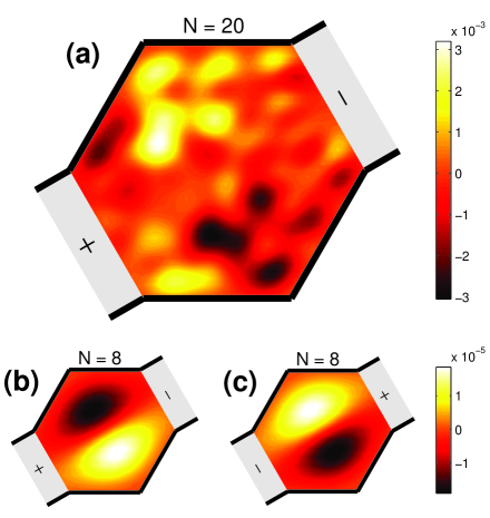
Figure 2: (Color online) Non-equilibrium spin-Hall accumulation $\left\langle S_{z}\right\rangle$ in a (a) $N=20$ sample under high bias, and a (b) $N=8$ sample under low bias. (c) is the same as (b), except the reversed bias. The color bars calibrate $\left\langle S_{z}\right\rangle$ in units of $\hbar/2$, and $\pm$ signs indicate the applied bias $\pm eV/2$ on the corresponding lead.

When reducing the sample size to $N=8$, one can see that the accumulation pattern changes sign, as shown in Fig. 2(b), where low bias is applied. This is because the spin-orbit forceSOforce depends on not only the sign of $S_{z}$, but also the system size relative to the Rashba spin precession lengthHaoPL

$$L_{\text{SO}}\equiv\frac{\pi\hbar^{2}}{2m^{\star}\alpha}=\frac{\pi at_{0}}{2t^{R}},$$ (16)

which is the distance required by the RSO interaction to rotate the spin by $\pi$. With $t^{R}=0.1t_{0}$ here, Eq. (16) yields the precession length $L_{\text{SO}}=5\pi a\approx 15.7a$. We will address this accumulation reversal effect a bit further later. Upon reversing the bias, Fig. 2(c) shows a flipped pattern, as expected. In short, Fig. 2 can be regarded as the hexagonal version of Fig. 1 shown in Ref. Nikolic, , and the general feature of the intrinsic SHE is preserved.

IV.2 SHA: Symmetry investigation

From now on we focus on the low-bias regime and, in this subsection, we put emphasis on different lead configurations. Various $N=12$ samples with 2 leads, 4 leads, and 6 leads with different configurations will be shown.

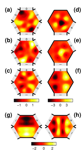
Figure 3: (Color online) Spin-Hall accumulation in $N=12$ hexagonal samples with (a)–(c) 6 leads, (d)–(f) 2 leads, and (g)–(h) 4 leads, under low bias. In addition to the $\pm$ signs indicating the applied $\pm eV/2$ bias, the zero signs in (a)–(c) label the unbiased leads. Color bars calibrate $\left\langle S_{z}\right\rangle$ in units of $\left(\hbar/2\right)\times 10^{-5}$.

Beginning with the 6-lead cases, Figs. 3(a)–3(c) show SHA patterns under a series of different biasing. For the non-head-to-tail biasing in Figs. 3(a) and 3(b), one can see a curved spin-Hall symmetry which roughly follows the charge current flow. Moreover, such a bent SHA may induce $\left\langle S_{z}\right\rangle$ on edges with not necessarily the opposite signs, e.g., see the dark spots in the left-top and right-bottom corners shown in Fig. 3(a). For the head-to-tail-biased sample of Fig. 3(c), the straight spin-Hall symmetry is recovered, as expected. As a direct correspondence, we unplug those unbiased electrodes and show the accumulation patterns in Figs. 3(d)–(f). Similar properties mentioned above are still valid, but each pattern becomes totally different, implying that the spin accumulation is sensitively affected by the configuration of attached leads.

We now focus on Figs. 3(c) and 3(f) and discuss the SHARE for these two distinct cases: open vs. closed boundaries. For the open case Fig. 3(c), one can clearly observe that the accumulation pattern reverses with different transverse length, which ranges from $\left(N-1\right)a=11a$ (the hexagon edge length) to $2\left(N-1\right)a=22a$ (the maximal length of the hexagon) here and covers the precession length $L_{\text{SO}}=15.7a$. Near the biased top and bottom electrodes, the spin accumulation signs can be well explained by the semiclassical SO force (to be discussed further later) proportional to $\left(\mathbf{p}\times\mathbf{e}_{z}\right)\otimes\sigma_{z}$ [see Eq. (18) in Sec. IV.3], which predicts right deflection for $\sigma_{z}=+1$ and left deflection for $\sigma_{z}=-1$. At central regions where the transverse length exceeds $L_{\text{SO}}$, the Rashba spin precession turns $\sigma_{z}=\pm 1$ into $\sigma_{z}=\mp 1$ and thus flips the pattern.

For the closed case Fig. 3(f), the SHARE is slightly different, as one can see that the bright and dark regions do not swap locally. A basic difference between the open and closed cases is that the electron does not have the outflow degree of freedom in the latter case. Therefore, the criterion of whether the pattern is flipped or not lies on the maximum width of the whole sample, which amounts to $22a$ for this $N=12$ case and exceeds $L_{\text{SO}}$ already. Accordingly, the SO force predicts right (left) deflection for $\sigma_{z}=-1$ ($\sigma_{z}=+1$) electrons, in agreement with Fig. 3(f). Indeed, the critical size for the closed sample (with two head-to-tail leads) to exhibit the flipped accumulation patterns can be shown as $N=9$, but we do not further show here.

Figures 3(g) and 3(h) show accumulation patterns in the hexagon sample attached by 4 leads with two different bias configurations. As in the former case longitudinal bias is arranged similar to the rectangular sample attached to two leads, regular spin-Hall accumulation is observed in Fig. 3(g). Interestingly, when we rearrange the applied bias as that in Fig. 3(h), “local” SHA is obtained: spin accumulation in the whole sample is divided into two parts, subject to the two separate pairs of positive-negative electrodes. The reason to obtain such a divided accumulation pattern can be intuitively understood as that each pair of the electrodes are closely connected, so that electron spins flow directly from “$+$” to “$-$” at one side and are less affected by the electrode pair at the other side.

A last remarkable point for Fig. 3 is the order of magnitude of $\left\langle S_{z}\right\rangle$. Strictly speaking, one should refer the local spin density $\left\langle S_{z}\right\rangle$ to the spin accumulation only for those patterns in closed samples. When attaching unbiased transverse leads, electrons are free to leak out, such that the local spin density shows merely the spatial spin distribution. It is only when the leads at the transverse sides are unplugged that those spins deflected by the SO force accumulate at the transverse edges and that the local spin density showing obvious peaks near the edges deserve the name spin-Hall accumulation. In addition, such a leakage of the spins due to plugged leads (not necessary unbiased) may lower the order of magnitude of $\left\langle S_{z}\right\rangle$ as can be clearly seen by comparing the three groups in Figs. 3: (a)–(c), (d)–(f), and (g)–(h).

IV.3 Competition forces in-between Rashba and Dresselhaus interactions

The semiclassical force provides a simple description of the SHE. Using the Heisenberg equation of motion with Hamiltonian $\mathcal{H}$ given by Eqs. (1)–(3), the velocity can be obtained as

$$\mathbf{v} =\mathbf{\dot{r}=}\frac{1}{i\hbar}\left[\mathbf{r},H\right]$$

$$=\frac{\mathbf{p}}{m^{\star}}+\frac{1}{\hbar}\left[\left(-\alpha\sigma_{y}+\beta\sigma_{x}\right)\mathbf{e}_{x}+\left(\alpha\sigma_{x}-\beta\sigma_{y}\right)\mathbf{e}_{y}\right],$$ (17)

leading to the SO-coupling-induced force

$$\mathbf{F}_{\text{SO}}\equiv m^{\star}\mathbf{\dot{v}=}\frac{m^{\star}}{i\hbar}\left[\mathbf{v},H\right]=\frac{2m^{\star}}{\hbar^{3}}\left(\alpha^{2}-\beta^{2}\right)\left(\mathbf{p\times e}_{z}\right)\sigma_{z}.$$ (18)

Apart from the constant prefactor $2m^{\star}/\hbar^{3}$, three transparent properties of $\mathbf{F}_{\text{SO}}$ given by Eq. (18) can be identified. First, spin-up electrons ($\sigma_{z}=+1$) and spin-down electrons ($\sigma_{z}=-1$) feel opposite forces. Second, since $\mathbf{F}_{\text{SO}}$ is always perpendicular to the electron transport direction [$\mathbf{F}_{\text{SO}}\propto\left(\mathbf{p\times e}_{z}\right)\perp\mathbf{p}$], no work is done by this force. In other words, the spin current caused by $\mathbf{F}_{\text{SO}}$ is dissipationless. Third, the Rashba and Dresselhaus interactions contribute oppositely to $\mathbf{F}_{\text{SO}}$, such that they compete against each other. Thus the sign of $\mathbf{F}_{\text{SO}}$ is also governed by $\left(\alpha^{2}-\beta^{2}\right)$, implying a reverse of the entire accumulation pattern when interchanging $\alpha$ with $\beta$.

To demonstrate this SHARE due to the exchange of $\left(\alpha,\beta\right)\leftrightarrow\left(\beta,\alpha\right)$, or $\left(t^{R},t^{D}\right)\leftrightarrow\left(t^{D},t^{R}\right)$, let us consider again the low-biased $N=12$ hexagonal samples with two head-to-tail leads. We show SHA patterns for various $\left(t^{R},t^{D}\right)$ in Fig. 4, where the left and right columns are related by interchanging $t^{R}$ and $t^{D}$, and the SHARE induced by the DSO coupling is clearly seen: patterns with $\left(t^{R},t^{D}\right)\leftrightarrow\left(t^{D},t^{R}\right)$ are reversal of each other. One can also observe that whereas we put $t^{R}>t^{D}$ in the left column and $t^{R}<t^{D}$ in the right column, the reversed patterns mean the exchange between the spin-up and spin-down states, implying a sign change in the spin-Hall conductivity as previously predicted.Sinova2

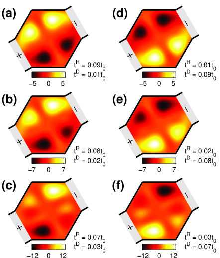
Figure 4: (Color online) Spin-Hall accumulation $\left\langle S_{z}\right\rangle$ in units of $\left(\hbar/2\right)\times 10^{-5}$ for $N=12$ hexagonal samples, each with two head-to-tail leads under low bias, for various $t^{R}$’s and $t^{D}$’s. Left column (a)–(c) and right column (d)–(f) are related by interchanging $t^{R}$ and $t^{D}$.

Another interesting point is that the coexistence of the RSO and DSO couplings breaks the spin-Hall symmetry. When one of $t^{R}$ or $t^{D}$ dominates, such as Figs. 4(a) or 4(d), the SHA on one side is (nearly) an mirror (with different sign) of that on the other side; while the magnitude of $t^{R}$ and $t^{D}$ becomes competitive, such as Figs. 4(c) or 4(f), the spin-Hall symmetry is broken, or distorted. Interestingly, this distortion effect does not simply kill the SHA pattern. Instead, the spin accumulation on only one side becomes vague while that on the other side becomes even stronger, as shown in Figs. 4(c) or 4(f). However, for systems with $t^{R}\approx t^{D}$ vanishing $\left\langle S_{z}\right\rangle$ inside the 2DEG is obtained (not shown here), as already implied in Eq. (18).

V Concluding remarks

In conclusion, the intrinsic SHE in hexagon-shaped 2DEG is investigated. The tight-binding model in triangular lattice which suits the hexagon edges is constructed (within the long wave length limit) for the linear Rashba and Dresselhaus [001] models. Applying the derived Hamiltonian (with matrix elements summarized in Table 1) to the LK formalism, we have shown the SHA patterns in hexagonal samples under various conditions, including SO interaction strength, bias strength, sample size, lead configuration, and SO interaction types. The spin-Hall symmetry is identified and discussed in detail, while the reversal effect of the SHA pattern, which may be induced by the sample size and the competition between the RSO and DSO couplings, are discussed. Contrary to the SHA in rectangular samples, we demonstrate here that the accumulation pattern can be very different due to the geometry effect.

Before closing, three remarks are worthy of mention here. First we highlight again the main difference between the hexagonal and the rectangular samples. Although bending the spin-Hall symmetry by applying non-straight biasing can be done in the rectangular case, transport angles with multiples of 90 degrees lowered to 60 enlarge the option of lead configuration. Explicitly, the total number of ways of biasing the sample, e.g., for the two-lead case, is increased from $C_{2}^{4}=6$ to $C_{2}^{6}=15$, making more detailed analysis possible. (Note that in general, samples should be treated as crystallography-dependent, so that each biasing direction is nontrivial.) In addition, the oblique side boundary varying with longitudinal position making the SHARE observable [Fig. 3(c)]. Such a reversal due to spin precession cannot be observed in one single rectangular sample.

Secondly, we remark on the sample size dependence. There are two characteristic lengths relavant in our hexagonal samples: spin precession length $L_{\text{SO}}$ and Fermi wave length $\lambda_{F}$. As we have discussed the spin-orbit force, the former is the sign criterion of the spin accumulation pattern. As long as the device size is larger than $L_{\text{SO}}$, the direction of the spin-orbit force, and hence the sign of $\left\langle S_{z}\right\rangle$ accumulating at the two sides, oscillate with the increase of the sample size. The latter, $\lambda_{F}$, modulates the spatial distribution of $\left\langle S_{z}\right\rangle$ and thus induces additional peaks similar to the standing waves. This means that in samples with the dimension of the order of or larger than $\lambda_{F},$ such waves can be observed. In our calculations, we have $E_{F}-E_{b}=0.2t_{0}\approx 17$ m$\operatorname{eV}$ and thus $\lambda_{F}=2\pi\hbar/\sqrt{2m^{\star}E_{F}}\approx 13a$, which is slightly shorter than $L_{\text{SO}}$. A good example is to compare Fig. 2(b) and Fig. 3(f). Under exactly the same conditions (lead configuration, bias strength, etc.), the former with $N=8$ shows no additional peaks, while in the latter with $N=12$ the $\left\langle S_{z}\right\rangle$ distribution exhibits two peaks at each side due to wave function modulation.

Finally, we stress again the nature of our calculation. It is the hexagonal boundary that makes discretizing the two-dimensional space inside the sample into a triangular lattice necessary. In the long wave length limit, where the Fermi energy is close to the band bottom so that crystal structure information is less important, our calculation simply reveals the free electron gas behavior. It is only when the Fermi level no longer approaches the band bottom that the band structure effect enters and the realistic crystal structure needs be taken.

Our present work provides a fundamental description of the geometry effect on the intrinsic SHE, taking the hexagon as the specific case. Additional degrees of freedom on configuring the attached leads may imply alternative ways of manipulating spins and even other spin-Hall experiment setups.

- (1) S. A. Wolf, D. D. Awschalom, R. A. Buhrman, J. M. Daughton, S. von Molnár, M. L. Roukes, A. Y. Chtchelkanova, and D. M.Treger, Science 294, 1488 (2001).
- (2) G. A. Prinz, Science 282, 1660 (1998).
- (3) M. I. D’yakonov and V.I. Perel’, Zh. Eksp. Teor. Fiz. 13, 657 (1971) [Sov. Phys. JEPT 33, 467 (1971)].
- (4) J. E. Hirsch, Phys. Rev. Lett. 83, 1834 (1999).
- (5) S. Zhang, Phys. Rev. Lett. 85, 393 (2000).
- (6) Wang-Kong Tse, J. Fabian, I. Žutić, and S. Das Sarma, Phys. Rev. B. 72, 241303(R) (2005)
- (7) Y. K. Kato, R. C. Myers,A. C. Gossard, D. D. Awschalom, Science 306, 1117 (2004); J. Wunderlich, B. Kaestner, J. Sinova, and T. Jungwirth, Phys. Rev. Lett. 94, 047204 (2005); V. Sih, R.C. Myers, Y. K. Kato, W.H. Lau, A. C. Gossard, D. D. Awschalom, Nature Phys. 1, 31(2005); B. Kaestner, J. Wunderlich, T. Jungwirth, J. Sinova, K. Nomura, A. H. MacDonald, Phys. E. 34, 47(2006).
- (8) S. Murakami, N. Nagaosa, and S. C. Zhang, Science 301, 1348 (2003)
- (9) S. Murakami, N. Nagaosa, and S. C. Zhang, Phys. Rev. B 69, 235206 (2004).
- (10) S. Murakami, Phys. Rev. B 69, 241202(R) (2004).
- (11) D. Culcer, J. Sinova, N. A. Sinitsyn, T. Jungwirth, A. H. MacDonald, and Q. Niu, Phys. Rev. Lett. 93, 046602 (2004).
- (12) L. Hu, J. Gao, and S.-Q. Shen, Phys. Rev. B 70, 235323 (2004).
- (13) G. Y. Guo, Yugui Yao, and Q. Niu, Phys. Rev. Lett. 94, 226601 (2005).
- (14) J. Schliemann and D. Loss , Phys. Rev. B 69, 165315 (2004).
- (15) A. A. Burkov, Alvaro S. Nunez, and A. H. MacDonald, Phys. Rev. B 70, 155308 (2004).
- (16) S.-Q. Shen, M. Ma, X. C. Xie, and F. C. Zhang, Phys. Rev. Lett. 92, 256603 (2004).
- (17) S.-Q. Shen, Phys. Rev. B. 70, 081311(R) (2004).
- (18) Ming-Che Chang, Phys. Rev. B 71, 085315 (2005).
- (19) J. Sinova, D. Culcer, Q. Niu, N.A. Sinitsyn, T. Jungwirth, and A.H. MacDonald, Phys. Rev. Lett. 92, 126603 (2004).
- (20) N. A. Sinitsyn, E. M. Hankiewicz, W. Teizer, and J. Sinova, Phys. Rev. B 70, 081312(R) (2004).
- (21) L. Sheng, D. N. Sheng, and C. S. Ting, Phys. Rev. Lett. 94, 016602 (2005).
- (22) B. K. Nikolić, S. Souma, L. P. Zârbo, and J. Sinova, Phys. Rev. Lett. 95, 046601 (2005).
- (23) B. K. Nikolić, L. P. Zârbo, and S. Souma, Phys. Rev. B 73, 075303 (2006).
- (24) B. K. Nikolić, L. P. Zârbo, and S. Welack, Phys. Rev. B 72, 075335 (2005).
- (25) B. K. Nikolić, L. P. Zârbo, and S. Souma, Phys. Rev. B 72, 075361 (2005).
- (26) K. Nomura, J. Wunderlich, J. Sinova, B. Kaestner, A. H. MacDonald, and T. Jungwirth, Phys. Rev. B 72, 245330 (2005).
- (27) J. Wang and K. S. Chan, Phys. Rev. B 72, 045331 (2005).
- (28) K. Hattori and H. Okamoto, Phys. Rev. B 74, 155321 (2006).
- (29) E.I. Rashba, Sov. Phys. Solid State 2, 1109 (1960).
- (30) J. Nitta, T. Akazaki, H. Takayanagi, and T. Enoki, Phys. Rev. Lett. 78, 1335 (1997).
- (31) B. Das, D.C. Miller, S. Datta, R. Reifenberger, W.P. Hong, P.K. Bhattacharya, J. Singh, and M. Jaffe, Phys. Rev. B 39, R1411 (1989).
- (32) G. Dresselhaus, Phys. Rev. 100, 580 (1955).
- (33) G. Lommer, F. Malcher, and U. Rössler, Phys. Rev. B 32, R6965 (1985); Yu. A. Bychkov and E. I. Rashba, in Proceedings of the 17th International Conference on Physics of Semiconductors, San Francisco, 1984 (Springer, New York, 1985), p. 321; M. I. D’yakonov and V. Y. Kachorovskii, Sov. Phys. Semicond. 20, 110 (1986).
- (34) M. I. D’yakonov and V. I. Perel’, Sov. Phys. JETP 33, 1053 (1971).
- (35) G. Bastard and R. Ferreira, Surf. Sci. 267, 335 (1992).
- (36) Supriyo Datta, Electronic transport in mesoscopic systems (Cambridge University Press, Cambridge, 1995).
- (37) L. V. Keldysh, Sov. Phys. JETP 20, 1018 (1965).
- (38) C. Caroli, R. Combescot, P. Nozieres, and D. Saint-James, J. Phys. C 4, 916 (1971).
- (39) P. Danielewicz, Ann. Phys. (N.Y.) 152, 239 (1984).
- (40) Robert van Leeuwen, Nils Erik Dahlen, Gianluca Stefanucci, Carl-Olof Almbladh, and Ulf von Barth, e-print arXiv:cond-mat/0506130.
- (41) Ming-Hao Liu and Ching-Ray Chang, Phys. Rev. B 74, 195314 (2006).