Algebraic vortex liquid theory of a quantum antiferromagnet on the kagome lattice

Abstract

There is growing evidence from both experiment and numerical studies that low half-odd integer quantum spins on a kagome lattice with predominant antiferromagnetic near neighbor interactions do not order magnetically or break lattice symmetries even at temperatures much lower than the exchange interaction strength. Moreover, there appear to be a plethora of low energy excitations, predominantly singlets but also spin carrying, which suggest that the putative underlying quantum spin liquid is a gapless “critical spin liquid” rather than a gapped spin liquid with topological order. Here, we develop an effective field theory approach for the spin-1/2 Heisenberg model with easy-plane anisotropy on the kagome lattice. By employing a vortex duality transformation, followed by a fermionization and flux-smearing, we obtain access to a gapless yet stable critical spin liquid phase, which is described by (2+1)-dimensional quantum electrodynamics (QED₃) with an emergent $\mathrm{SU}(8)$ flavor symmetry. The specific heat, thermal conductivity, and dynamical structure factor are extracted from the effective field theory, and contrasted with other theoretical approaches to the kagome antiferromagnet.

I introduction

Kagome antiferromagnets are among the most extreme examples of frustrated spin systems realized with nearest-neighbor interactions. Both the frustration in each triangular unit and the rather loose “corner-sharing” aggregation of these units into the kagome lattice suppress the tendency to magnetically order. On the classical level, kagome spin systems are known to exhibit rather special properties: nearest-neighbor Ising and XY models remain disordered even in the zero-temperature limit, while the $\mathrm{O}(3)$ system undergoes order-by-disorder into a coplanar spin structure.Huse92

Quantum kagome antiferromagnets, which are much less understood, provide a fascinating arena for the possible realization of spin liquids. Early exact diagonalization and series expansion studiesZeng90 ; Singh92 ; Leung93 ; Elstner94 as well as further exhaustive numerical works, Lecheminant97 ; Waldtmann98 ; Sindzingre00 ; Misguich05 provide strong evidence for the absence of any magnetic order or other symmetry breaking in the nearest neighbor spin-1/2 system. Moreover, a plethora of low energy singlet excitations is found, below a small (if non-zero) spin gap. But the precise nature of the putative spin liquid phase in this model has remained elusive.

On the experimental front, several quasi-two dimensional materials with magnetic moments in a kagome arrangement have been studied, including SrCr_8-xGa_4+xO₁₉ with Cr³⁺ ($S=3/2$) momentsObradors88 ; Ramirez90 ; Broholm90 ; Ramirez92 ; Ramirez00 , jarosites KM₃(OH)₆(SO₄)₂ with M$=$Cr³⁺ or Fe³⁺ ($S=5/2$) momentsWills01 ; Inami00 ; Lee97 , and volborthite Cu₃V₂O₇(OH)${}_{2}\cdot$ 2H₂O with Cu²⁺ ($S=1/2$) momentsHiroi01 . Recently, herbertsmithite ZnCu₃(OH)₆Cl₂ which also has Cu²⁺ moments on a kagome lattice was synthesized for which no magnetic order is observed down to 50 mK despite the estimated exchange constant of 300 K. Helton06 ; Ofer06 ; Mendels06 The second layer of ³He absorbed on graphoile is also believed to realize the kagome magnet.Masutomi04 ; Elser89 The suppression of long-range spin correlations or other signs of symmetry breaking down to temperatures much lower than the characteristic exchange energy scale is manifest in all of these materials, consistent with expectations. Moreover, there is evidence for low energy excitations, both spin carrying and singlets. But the ultimate zero-temperature spin liquid state is often masked in these systems by magnetic ordering or glassy behavior at the lowest temperatures, perhaps due to additional interactions or impurities, rendering the experimental study of the spin liquid properties problematic. New materials and other experimental developments are changing this situation, and the question of the quantum spin liquid ground state of the kagome antiferromagnet is becoming more prominent.

There are two broad classes of spin liquids which have been explored theoretically, both in general terms and for the kagome antiferromagnet in particular. The first class comprise the “topological” spin liquids, which have a gap to all excitations and have particle-like excitations with fractional quantum numbers above the gap. Arguably, the simplest topological liquids are the so-called $Z_{2}$ spin liquids, which support a vortex like excitation - a vison - in addition to the spin one-half spinon. For the kagome antiferromagnet, Sachdev Sachdev91 and more recently Wang and Vishwanath Wang06 have employed a Schwinger boson approach to systematically access several different $Z_{2}$ spin liquids. For a kagome antiferromagnet with easy axis anisotropy and further neighbor interactions, Balents et al.Balents02 unambiguously established the presence of a $Z_{2}$ spin liquid, obtaining an exact ground state wavefunction in a particular limit. Quantum dimer models on the kagome lattice can also support a $Z_{2}$ topological phaseMisguich02 . Spin liquids with topological order and time reversal symmetry breaking, the chiral spin liquids which are closely analogous to fractional quantum Hall states, have been found on the kagome latticeMarston91 ; KunYang93 within a fermionic representation of the spins. But all of these topological liquids are gapped, and cannot account for the presence of many low excitations found in the exact diagonalization studies and suggested by the experiments.

A second class of spin liquids - the “critical” or “algebraic spin liquids” (ASL) - have gapless singlet and spin carrying excitations. Although these spin liquids share many properties with quantum critical points such as correlation functions falling off as power laws with non-trivial exponents, they are believed to be stable quantum phases of matter. Within a fermionic representation of the spins, HastingsHastings01 explored an algebraic spin liquid on the kagome lattice, and more recently Ran et al.Ran06 have extended his analysis in an attempt to explain the observed properties of herbertsmithite ZnCu₃(OH)₆Cl₂.

In this paper, motivated by the experiments on the kagome materials and the numerical studies, we pursue yet a different approach to the possible spin liquid state of the kagome antiferromagnet. As detailed below, for a kagome antiferromagnet with easy-plane anisotropy we find evidence for a new critical spin liquid, an “algebraic vortex liquid” (AVL) phase. Earlier we had introduced and explored the AVL in the context of the triangular XXZ antiferromagnet in Refs. Alicea05, ; Alicea05a, ; Alicea05b, . Compared to the slave particle techniques for studying frustrated quantum antiferromagnets, the AVL approach is less microscopically faithful to a specific spin Hamiltonian, but has the virtue of being unbiased.

Our approach requires the presence of an easy-plane anisotropy, which for a spin one-half system can come from the Dzyaloshinskii-Moriya interaction, although this is usually quite small. But for higher half-integer spin systems, spin-orbit coupling allows for a single ion anisotropy $D(S^{z})^{2}$ which can be appreciable. With $D>0$ this leads to an easy-plane spin character, and from a symmetry stand point our analysis should be relevant. Moreover, a very interesting unpublished exact diagonalization study by Sindzingre Sindzingre suggests that an unusual spin liquid phase is also realized for the nearest-neighbor quantum XY antiferromagnet. He finds a small gap to $S^{z}=1$ excitations, but below this gap there is a plethora of $S^{z}=0$ states, which is reminiscent of the many singlet excitations below the triplet gap in the Heisenberg SU(2) spin model.Lecheminant97 Thus, based on the exact diagonalization studies, the easy plane anisotropy does not appear to gap out the putative critical spin liquid of the Heisenberg model, although it will presumably modify its detailed character.

Our approach to easy-plane frustrated quantum antiferromagnets focuses on vortex defects in the spin configurations, rather than the spins themselves. In this picture, the magnetically ordered phases do not have vortices present in the ground state. But there will be gapped vortices, and these can lead to important effects on the spectrum. For example, vortex-antivortex (i.e. roton) excitations can lead to minima in the structure factor at particular wavevectors in the Brillouin zone, Zheng06 ; Zheng06b ; Starykh in analogy to superfluid He-4. As we demonstrated for the triangular antiferromagnet and explore below for the kagome lattice, our approach predicts specific locations in the Brillouin zone for the roton minima, which could perhaps be checked by high order spin wave expansion techniques. On the other hand, the presence of mobile vortex defects in the ground state can destroy magnetic order, giving access to various quantum paramagnets. If the vortices themselves condense, the usual result is the breaking of lattice symmetries, such as in a spin Peierls state. But if the vortices remain gapless one can access a critical spin liquid phase.

For frustrated spin models the usual duality transformation to vortex degrees of freedom does not resolve the geometric frustration since the vortices are at finite density. However, by binding $2\pi$-flux to each vortex converting them into fermions coupled to a Chern-Simons gauge field followed by a simple flux-smearing mean-field treatment gives a simple way to describe the vortices. The long-range interaction of vortices actually works to our advantage here since it suppresses their density fluctuations and leads essentially to incompressibility of the vortex fluid. As demonstrated in the easy-plane quantum antiferromagnet on the triangular lattice,Alicea05a ; Alicea05b including fluctuations about the flux-smeared mean field enables one to access a critical spin liquid with gapless vortices. The theory has the structure of a (2+1)-dimensional [(2+1)D] quantum electrodynamics (QED₃), with relativistic fermionic vortices minimally coupled to a non-compact U(1) gauge field. The resulting algebraic vortex liquid (AVL) phase is a novel critical spin liquid phase that exhibits neither magnetic nor any other symmetry-breaking order. This approach also allows one to study many competing orders in the vicinity of the gapless phase.

When applied to the spin-1/2 easy-plane antiferromagnet on the kagome lattice, the duality transformation combined with fermionization and flux smearing also leads to a low-energy effective QED₃ theory with 8 flavors of Dirac fermions with an emergent $\mathrm{SU}(8)$ flavor symmetry. Amusingly, AVL’s with $\mathrm{SU}(2)$ Alicea05 , $\mathrm{SU}(4)$ Alicea05a ; Alicea05b and $\mathrm{SU}(6)$ Alicea06 emergent symmetries were obtained previously for quantum XY antiferromagnets on the triangular lattice, with integer spin, half-integer spin and half-integer spin in an applied magnetic field, respectively. QED₃ theory with $N$ flavors of Dirac fermions is known to realize a stable critical phase for sufficiently large $N>N_{c}$. While numerical attempts to determine $N_{c}$ are so far inconclusive,Hands02 ; Hands04 an estimate from the large-$N$ expansion suggests $N_{c}\sim 4$.Alicea05 It seems very likely that $N=8$ is large enough, implying the presence of a stable critical spin liquid ground state for the easy-plane spin-1/2 quantum antiferromagnet on the kagome lattice.

Although the algebraic vortex liquid and the algebraic spin liquidHastings01 ; Ran06 obtained for the kagome lattice are accessed in rather different ways, they share a number of commonalities, both theoretically and with regard to their experimental implications. Both approaches end with a QED₃ theory, the former a non-compact gauge field theory with fermionic vortices carrying an emergent SU(8) symmetry, and the latter a compact gauge theory with fermionic spinons with SU(4) symmetry. The non-compact nature of the gauge field in the AVL follows from the fact that the $S^{z}$ component of spin appears as the gauge flux in the dualized theory. Hence the states with zero flux and $2\pi$ flux are physically distinct; moreover, it follows that since the total $S^{z}$ is conserved, so also is the total gauge flux. This should be contrasted with the slave particle approach, where a compact gauge theory arises on the lattice and there is no such conservation law. Physically, this means that dynamical monopole operators, which could potentially destabilize the spin liquid and open a gap in the excitation spectrum, are not allowed in our low-energy theory for the AVL, while they are allowed in a low-energy description of spin liquids obtained using a slave particle framework.

With regard to experimentally accessible quantities, both theories predict a power law specific heat $C\sim T^{2}$ at low temperatures, which follows from the linear dispersion of the fermions, and which would dominate the phonon contribution to the specific heat for magnets with exchange interactions significantly smaller that the Debye frequency. remark specific heat Because the spinons couple directly to magnetic fields, one would expect the specific heat in the ASL to be more sensitive to an external applied magnetic field than the AVL phase. Both theories predict a thermal conductivity which vanishes as $\kappa\sim T$, Ioffe90 ; Lee92 which is an interesting experimental signature reflecting the dynamical mobility of the gapless excitations.

The momentum resolved dynamical spin structure factor which can be extracted from inelastic neutron experiments can in principle give very detailed information about the spin dynamics. Following the framework developed on the triangular lattice,Alicea05 ; Alicea05a ; Alicea05b ; Alicea06 for the kagome AVL we can extract the wavevectors in the magnetic Brillouin zone which have gapless spin carrying excitations, and find 12 of them as shown in Fig. 4. In contrast, the kagome ASL phase is predicted to have gapless spin excitations at only 4 of these 12 momenta. The momentum space location of the gapless excitations is perhaps the best way to try and distinguish experimentally between these two (and any other) critical spin liquids.

The rest of the paper is organized as follows. We start by introducing our model in Sec. II. The low-energy effective field theory is then developed in Sec. III. In Sec. IV, the properties of the critical spin liquid phase (AVL phase) are discussed, especially, the spin excitation (roton spectrum) (Fig. 5), the $S^{z}$ dynamical structure factor (Eq. 19), and the in-plane dynamical structure factor (Eq. 22). We conclude in Sec. V. Some details of the analysis are presented in three Appendices.

II Extended kagome Model

Our primary interest is the kagome lattice spin-1/2 model with easy-plane anisotropy (quantum XY model)

$$\mathcal{H} = \frac{1}{2}\sum_{\mathbf{r},\mathbf{r}^{\prime}}\left[J^{\ }_{\mathbf{r},\mathbf{r}^{\prime}}S^{+}_{\mathbf{r}}S^{-}_{\mathbf{r}^{\prime}}+\mathrm{h.c.}\right]+\sum_{\mathbf{r},\mathbf{r}^{\prime}}J^{z}_{\mathbf{r},\mathbf{r}^{\prime}}S^{z}_{\mathbf{r}}S^{z}_{\mathbf{r}^{\prime}},$$ (1)

with $J^{\ }_{\mathbf{r},\mathbf{r}^{\prime}}>J^{z}_{\mathbf{r},\mathbf{r}^{\prime}}$. We consider the system with dominant nearest-neighbor exchange $J_{1}$, but will also allow some second- and third-neighbor exchanges $J_{2}$ and $J_{3}$.

To set the stage, the model with only nearest-neighbor coupling has an extensive degeneracy of classical ground states, which is lifted by further-neighbor interactions. For example, with antiferromagnetic $J_{2}>0$, the so-called $q=0$ phase is stabilized (Fig. 1). On the other hand, for ferromagnetic $J_{2}<0$, the so-called $\sqrt{3}\times\sqrt{3}$ structure is the classical ground state (Fig. 1). These ordered phases are also realized in the quantum spin-1/2 Heisenberg model for large enough $J_{2}$Lecheminant97 , while the case with $J_{2}/J_{1}\simeq 0$ is most challenging as mentioned in the introduction.

The easy-plane spin system can be readily reformulated in terms of vortices. But in order to apply the fermionized vortex approach more simply, we consider a wider class of models which includes the nearest-neighbor kagome model. Specifically, we add one extra site at the center of each hexagon, on which we put an integer spin (Fig. 1). (Technical reasons for doing this are discussed at the end of Sec. III.) In the rotor representation of spins, with a phase $\varphi$ canonically conjugate to the integer boson number, $n\sim S^{z}+1/2$ on the kagome sites and $n\sim S^{z}$ at the centers of each hexagon, such an extended model reads

$$\mathcal{H} = \sum_{\mathbf{r},\mathbf{r}^{\prime}}J_{\mathbf{r},\mathbf{r}^{\prime}}\cos\left(\varphi_{\mathbf{r}}-\varphi_{\mathbf{r}^{\prime}}\right)+\sum_{\mathbf{r}}U_{\mathbf{r}}\left(n^{\ }_{\mathbf{r}}-n^{0}_{\mathbf{r}}\right)^{2},$$ (2)

where $n^{0}=1/2$ for the kagome lattice sites, while $n^{0}=0$ for the added hexagon center sites. We have dropped the $J^{z}$ term for simplicity since it amounts to a mere renormalization of the interactions in the effective field theory that we will derive. As shown in Fig. 1, we take the interaction to be $J$ for the nearest neighbor half-integer spins, while the coupling that connects integer and half-integer spins is $J^{\prime}$. When the on-site interaction $U$ is infinitely large, $U\to\infty$, there remain two low-energy states realizing the Hilbert space of a $S=1/2$ spin at the kagome sites, whereas the frozen sector with $n_{\mathbf{r}}=0$ is selected at the hexagon center sites. In the quantum rotor model, we “soften” this constraint and take $U$ to be finite.

The additional integer-spin degrees of freedom do not spoil any symmetries of the original model, which for the record include lattice translations, reflections, and rotations, as well as XY spin symmetries. If we integrate over the extra degrees of freedom, the model looks very close to the original one. For example, in the limit when $J^{\prime}\ll U$, we obtain the kagome model with additional ferromagnetic second and third neighbor exchanges $J_{2}=J_{3}=-(J^{\prime})^{2}/(2U)$, together with a renormalized nearest-neighbor exchange $J_{1}=J-(J^{\prime})^{2}/(2U)$. Such exchanges would slightly favor the $\sqrt{3}\times\sqrt{3}$ state in the classical limit, but as we will see, the spin liquid phase that we obtain by analyzing the extended kagome model will have enhanced correlations corresponding to both the $q=0$ and $\sqrt{3}\times\sqrt{3}$ phases that are nearby. Thus the small bias introduced by the added integer-spin sites appears to be not so important for the generic spin liquid phase that we want to describe.

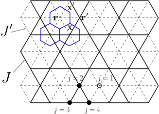
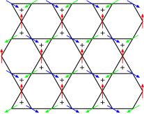
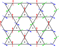
Figure 1: (Top) The quantum spin model with easy-plain anisotropy, Eq. (2), on the kagome lattice (thick line) supplemented by an extra site at the center of each hexagon. There is a half-integer spin for each kagome site whereas integer spins are placed at each center of hexagons. Four spins in a unit cell are labeled by $j=1,2,3,4$. For this triangular extension of the kagome lattice, the dual lattice is the honeycomb lattice indicated in the upper left part. (Bottom) The $q=0$ state (Left) and the $\sqrt{3}\times\sqrt{3}$ state (Right). Positive/negative vorticities (chiralities) for each triangle are denoted by $+/-$.

III Fermionized vortex description

The triangular extension of the kagome XY antiferromagnet discussed above is somewhat similar to the triangular lattice spin-1/2 XY antiferromagnet studied in Refs. Alicea05a, ; Alicea05b, , except that one quarter of the sites is occupied by integer spins. The duality transformation for the present model proceeds identically to Refs. Alicea05a, ; Alicea05b, , and turns the original spin Hamiltonian (2) into the dual Hamiltonian describing vortices hopping on the honeycomb lattice and interacting with a gauge field residing on the dual lattice links,

$$\mathcal{H} = 2\pi^{2}\sum_{\mathbf{x}\mathbf{x^{\prime}}}J_{\mathbf{x}\mathbf{x^{\prime}}}e^{2}_{\mathbf{x}\mathbf{x^{\prime}}}+\frac{U}{(2\pi)^{2}}\sum_{\mathbf{r}}\left(\nabla\times a\right)_{\mathbf{r}}^{2}$$ (3)

$$-2\sum_{\mathbf{x}\mathbf{x^{\prime}}}t_{\mathbf{x}\mathbf{x^{\prime}}}\cos\left(\theta_{\mathbf{x}}-\theta_{\mathbf{x^{\prime}}}-a^{\ }_{\mathbf{x}\mathbf{x}^{\prime}}-a^{0}_{\mathbf{x}\mathbf{x}^{\prime}}\right).$$

Here $\mathbf{x},\mathbf{x}^{\prime}$ label sites on the honeycomb lattice (see Fig. 1), $e^{\pm i\theta_{\mathbf{x}}}$ is a vortex creation/annihilation operator at site $\mathbf{x}$, and $a_{\mathbf{x}\mathbf{x}^{\prime}},e_{\mathbf{x}\mathbf{x}^{\prime}}$ represent a gauge field on the link connecting $\mathbf{x}$ and $\mathbf{x}^{\prime}$. $J_{\mathbf{x}\mathbf{x}^{\prime}}$ is given by $J_{\mathbf{x}\mathbf{x}^{\prime}}=J(J^{\prime})$ when the dual link $\langle\mathbf{x}\mathbf{x}^{\prime}\rangle$ crosses the original lattice link $\langle\mathbf{r}\mathbf{r}^{\prime}\rangle$ with $J_{\mathbf{r}\mathbf{r}^{\prime}}=J(J^{\prime})$. The last term in the dual Hamiltonian represents the vortex hopping where the hopping amplitude $t_{\mathbf{x}\mathbf{x}^{\prime}}$ is given by $t_{\mathbf{x}\mathbf{x}^{\prime}}=t(t^{\prime})$ when the link $\langle\mathbf{x}\mathbf{x}^{\prime}\rangle$ crosses the link $\langle\mathbf{r}\mathbf{r}^{\prime}\rangle$ with $J_{\mathbf{r}\mathbf{r}^{\prime}}=J(J^{\prime})$. Crudely, we have $t/t^{\prime}\sim J^{\prime}/J$ since vortices hop more easily across weak links (Fig. 2). Finally, the static gauge field $a^{0}$ encodes the average flux seen by the vortices when they move; this is described in more detail below.

In the dual description, because of the frustration in the spin model, the average density of vortices is one half per site. On the other hand, the original boson density is viewed as a gauge flux

$$n_{\mathbf{r}}=\frac{1}{2\pi}\left(\nabla\times\bm{a}\right)_{\mathbf{r}}=\frac{1}{2\pi}\sum_{\tiny\mbox{ $\langle\mathbf{x}\mathbf{x}^{\prime}\rangle$ around $\mathbf{r}$}}a_{\mathbf{x}\mathbf{x}^{\prime}}.$$ (4)

Therefore, vortices experience on average $\pi$ flux going around the triangular lattice sites with half-integer spins, but they see zero flux going around the sites with integer spins. Thus, one quarter of the hexagons will have zero flux as seen by the vortices, and this is where the present model departs from the considerations in Refs. Alicea05a, ; Alicea05b, .

To treat the system of interacting vortices at finite density, we focus on the two low-energy states with vortex number $N_{\bf x}=0$ and $N_{\bf x}=1$ at each site and view vortices as hard-core bosons. We can then employ the fermionization as in Refs. Alicea05a, ; Alicea05b, and arrive at the following hopping Hamiltonian for fermionized vortices $d_{\bf x}$

$$\mathcal{H}_{\mathrm{ferm}}=-\sum_{\mathbf{x}\mathbf{x^{\prime}}}\left[t_{\mathbf{x}\mathbf{x^{\prime}}}d^{{\dagger}}_{\mathbf{x}}d^{\ }_{\mathbf{x^{\prime}}}e^{-{i}\left(a_{\mathbf{x}\mathbf{x}^{\prime}}+a_{\mathbf{x}\mathbf{x}^{\prime}}^{0}+A_{\mathbf{x}\mathbf{x}^{\prime}}\right)}+\mathrm{h.c.}\right],$$ (5)

where we have introduced a Chern-Simons field $A$ whose flux is tied to the vortex density, $(\nabla\times A)_{\mathbf{x}}=2\pi N_{\mathbf{x}}$.

Before proceeding with the analysis of the fermionized vortex Hamiltonian, we now point out the technical reasons for considering the extended kagome model. If we apply the duality transformation to the kagome model with nearest-neighbor antiferromagnetic coupling $J_{1}$ only, we would obtain a dual vortex theory on the dice lattice, which is the dual of the kagome lattice. In this theory, in order to reproduce the rich physics while restricting the vortex Hilbert space at each site to something more manageable like the hard-core vortices described earlier, we would need to keep two low-energy states of vortices for each triangle of the kagome lattice (i.e., for each three-fold coordinated site of the dice lattice), whereas there are three such states to keep for each hexagon (i.e., six-fold coordinated dice site). The latter degrees of freedom are rather difficult to represent in terms of fermions. On the other hand, in the dual treatment of the extended model, such a six-fold coordinated dice lattice site is effectively split into six sites. Each such new site now has two low-energy states but the sites are coupled together, and this provides some caricature of the original important vortex states on the problematic dice sites. This representation now admits standard fermionization, and it was “found” in a rather natural way without any prior bias regarding how to treat the difficult dice sites with three important vortex states.

III.1 Flux smearing mean field and low energy effective theory

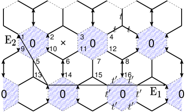
Figure 2: The flux-smeared mean field background for fermionized vortices. Each hexagon is threaded by either zero or $\pi$-flux. (hexagons with zero-flux are specified by “0” whereas all the other hexagons are pierced by $\pi$-flux.) A convenient choice of a gauge is also shown: for links labeled by $\leftrightarrow$, we assign the Peierls phase factor $e^{-{i}a^{0}_{\mathbf{x}\mathbf{x}^{\prime}}}=e^{{i}\pi}$. The unit cell in this gauge consists of 16 sites as labeled in the figure. For links represented by a solid line we assign hopping amplitude $t(=1)$ whereas for links denoted by a broken line we assign hopping $t^{\prime}$ . We take $\times$ in the figure as an origin.

The flux attachment implemented above is formally exact, and there have been no approximations so far, although we have softened the discreteness constraints on the gauge fields. To arrive at a low-energy effective field theory, we now pick a saddle point configuration of the gauge field, incorporating a flux-smeared mean-field ansatz, and later will include fluctuations around it. That is, we first distribute (or “smear”) the $2\pi$ flux attached to each vortex on a dual site to the three (dual) plaquettes surrounding it. Since the vortices are at half filling and each hexagon contains six sites, the total smeared flux through each hexagon is $2\pi$, which is equivalent to no additional flux. Therefore we assume $A_{\mathbf{x}\mathbf{x}^{\prime}}=0$ in the mean field. Also, we take $a_{\mathbf{x}\mathbf{x}^{\prime}}=0$ on average, including the fluctuations after we identify the important low-energy degrees of freedom for the fermionic vortices. Thus, at the mean field level, the original Hamiltonian (2) is converted into a problem of fermions hopping on the honeycomb lattice,

$$\mathcal{H}_{\mathrm{ferm,MF}} = \sum_{\mathbf{x}\mathbf{x^{\prime}}}\left[t_{\mathbf{x}\mathbf{x}^{\prime}}e^{-{i}a^{0}_{\mathbf{x}\mathbf{x}^{\prime}}}d^{{\dagger}}_{\mathbf{x}}d^{\ }_{\mathbf{x}^{\prime}}+\mathrm{h.c.}\right].$$ (6)

In the mean field, 3 out of 4 hexagons are pierced by $\pi$-flux, while the remaining hexagons with an integer spin at the center have zero flux, see Fig. 2. Our choice of the gauge is shown in Fig. 2. The unit cell consists of 16 sites, the area of which is twice as large as the physical unit cell of the original kagome spin system.

This Hamiltonian can be solved easily by the Fourier transformation. The lattice vectors that translate the unit cell are given by

$$\mathbf{E}_{1}=\big{(}4,0\big{)},\quad\mathbf{E}_{2}=\big{(}-1,\sqrt{3}\big{)}.$$ (7)

and the first Brillouin zone (BZ) is specified as the Wigner-Seitz cell of the reciprocal lattice vectors

$$\mathbf{G}_{1}=\left(\frac{\pi}{2},\frac{\pi}{2\sqrt{3}}\right),\quad\mathbf{G}_{2}=\left(0,\frac{2\pi}{\sqrt{3}}\right).$$ (8)

This is shown in Fig. 3. Note that, on the other hand, the physical unit cell is defined by $\mathbf{E}_{1}^{\mathrm{phys}}=\mathbf{E}_{1}/2=\left(2,0\right),$ and $\mathbf{E}_{2}^{\mathrm{phys}}=\mathbf{E}_{2}=\left(-1,\sqrt{3}\right).$ Thus the physical BZ is determined as the Wigner-Seitz cell of the reciprocal lattice vectors $\mathbf{G}^{\mathrm{phys}}_{1}=\left(\pi,\pi/\sqrt{3}\right)$ and $\mathbf{G}^{\mathrm{phys}}_{2}=\left(0,2\pi/\sqrt{3}\right)$, and is also shown in Fig. 3 and Fig. 4.

Because of the particle-hole symmetry of the original quantum rotor Hamiltonian, which in terms of the fermionized vortices is realized as a vortex particle-hole symmetry (see Appendix B), the band structure of the flux-smeared mean-field Hamiltonian (6) is symmetric around zero energy, and consists of eight bands with positive energy and eight with negative energy. The 7th and 8th bands have negative energy spectra and are completely degenerate,Vafek each having four Fermi points $\mathbf{Q}_{1,2,3,4}$ that touch zero energy. In the same way, the 9th and 10th bands have positive energy spectra and are completely degenerate, and each of them touches zero energy at the same four Fermi points $\mathbf{Q}_{1,2,3,4}$ thus completing the Dirac nodal spectrum. With the gauge choice specified in Fig. 2, the locations of the Fermi points in the BZ are

$$\mathbf{Q}_{1}=-\mathbf{Q}_{3} = \left(\frac{\pi}{12},\frac{\pi}{4\sqrt{3}}\right),$$ (9)

$$\quad\mathbf{Q}_{2}=-\mathbf{Q}_{4} = \left(\frac{\pi}{12},-\frac{3\pi}{4\sqrt{3}}\right),$$ (10)

(see Fig. 3). The low-energy spectrum consists of eight gapless two-component Dirac fermions with identical Fermi velocities given by (here we take $t=1$ for convenience)

$$v_{F}=\sqrt{\frac{6t^{\prime 2}}{(3+t^{\prime 2})(3+2t^{\prime 2})}}~{}.$$ (11)

Hence the low-energy effective theory enjoys an emergent $\mathrm{SU}(8)$ symmetry among eight Dirac cones, which is protected at the kinetic-energy level by the underlying discrete symmetries in the problem (see Appendix C).

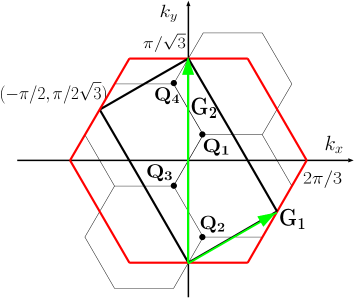
Figure 3: The first Brillouin zone for the flux smeared mean field ansatz and the location of the nodes $\mathbf{Q}_{1,\ldots,4}$. The hexagonal physical Brillouin zone is also presented. Small hexagons are guide for eyes.

The lattice fermionized vortex operator is conveniently expanded in terms of slowly varying continuum fields $\psi^{\ }_{i\alpha a}(\mathbf{x})$ by

$$d_{\mathbf{x}} \sim \sum_{\alpha=1}^{4}\sum_{i=\mathrm{I},\mathrm{II}}\sum_{a=1,2}e^{{i}\mathbf{Q}_{\alpha}\cdot\mathbf{x}}\phi^{\ }_{i\alpha a}(n)\,\psi^{\ }_{i\alpha a}(\mathbf{x}),$$ (12)

where indices $\alpha=1,\dots,4$, $i=\mathrm{I},\mathrm{II}$, and $a=1,2$, refer to the four Fermi momenta, two sublattices of the honeycomb lattice, and two degenerate bands, respectively, while $n=1,\dots,16$ specifies the site label in the unit cell, cf. Fig. 2. The 16-component wavefunctions $\phi^{\ }_{i\alpha a}(n)$ represent modes at the Fermi points and are specified in Appendix A.

Working with these continuum fields, we find that the low-energy Hamiltonian has the same form $v_{F}(-\sigma^{1}\hat{p}_{x}+\sigma^{2}\hat{p}_{y})$ near each Dirac node, where $\sigma^{1,2,3}$ are Pauli matrices that act on the “Lorentz” indices $i=\mathrm{I},\mathrm{II}$. Correspondingly, by introducing the gamma matrices in $(2+1)$D

$$\gamma_{0}=\sigma^{3},\quad\gamma_{1}=-\sigma^{2},\quad\gamma_{2}=-\sigma^{1},$$

$$\gamma_{\mu}\gamma_{\nu}+\gamma_{\nu}\gamma_{\mu}=2\delta_{\mu\nu},\quad\mu,\nu=0,1,2,$$ (13)

the Euclidean low-energy effective action is given by

$$S_{\mathrm{eff}} = \int d^{3}x\sum_{(\alpha)=1}^{8}\bar{\psi}^{\ }_{(\alpha)}\,\gamma_{\mu}\partial_{\mu}\psi^{\ }_{(\alpha)}$$ (14)

where $(\alpha)=\alpha a$ is a collective index running from 1 to 8; $x^{\mu=0,1,2}$ represents imaginary time as well as spatial coordinates; $\bar{\psi}=\psi^{{\dagger}}\gamma_{0}$; and we have scaled out $v_{F}$.

Having identified the low-energy fermionic degrees of freedom, we now reinstate gauge field fluctuations. The complete effective action is that of SU(8) QED₃ coupled in addition with the Chern-Simons field $A^{\ }_{\mu}$ and given by

$$S_{\mathrm{eff}}=\int d^{3}x\,\Biggr{[}\sum_{(\alpha)=1}^{8}\bar{\psi}^{\ }_{(\alpha)}\gamma_{\mu}\left(\partial_{\mu}-{i}a_{\mu}-{i}A_{\mu}\right)\psi^{\ }_{(\alpha)}$$

$$\quad+\mathcal{L}_{2f}+\mathcal{L}_{4f}+\frac{1}{2e^{2}}\left(\epsilon^{\ }_{\mu\nu\lambda}\partial^{\ }_{\nu}a^{\ }_{\lambda}\right)^{2}+\frac{{i}}{4\pi}\epsilon^{\ }_{\mu\nu\lambda}A^{\ }_{\mu}\partial^{\ }_{\nu}A^{\ }_{\lambda}\Biggl{]}.$$

(15)

Here we also included possible fermion bilinears $\mathcal{L}_{2f}$ and four fermion interactions $\mathcal{L}_{4f}$. $e^{2}\sim U^{-1}$ stands for the coupling constant of the gauge field $a_{\mu}$.

As discussed in Refs. Alicea05a, ; Alicea05b, , the Chern-Simons field $A_{\mu}$ is irrelevant. The microscopic symmetries of the spin Hamiltonian prohibit fermion mass terms $\mathcal{L}_{2f}$ from appearing in the effective action (see Appendix C). Furthermore, four fermion interactions $\mathcal{L}_{4f}$ in Eq. (15) are irrelevant when the number of fermion flavors is large enough, $N>N_{c}$. Thus, provided $N_{c}<8$, we have obtained a stable Algebraic Vortex Liquid phase that is described by QED₃ with an emergent $\mathrm{SU}(8)$ symmetry. Using the available theoretical understanding of such theories, we will now describe the main properties of the AVL phase, which in terms of the original spins is a gapless spin liquid phase.

IV Properties of the AVL phase

IV.1 Roton spectrum

First note that the specific momenta of the Dirac points Eq. (10) and Fig. 3 are gauge-dependent. We are interested in the physical properties of the system, which are gauge invariant. One such property is the vortex-antivortex excitation spectrum: By moving a vortex from an occupied state ${\bf k}$ with energy $E^{-}(\mathbf{k})$ to an unoccupied state $\mathbf{k^{\prime}}$ with energy $E^{+}(\mathbf{k^{\prime}})$, we are creating an excitation that carries energy $E^{+}(\mathbf{k^{\prime}})-E^{-}(\mathbf{k})$. Some care is needed if we want to construct such a state with a definite momentum in the physical BZ, since we need to consider both $\mathbf{k^{\prime}}-\mathbf{k}$ and $\mathbf{k^{\prime}}-\mathbf{k}+\mathbf{G}_{1}$. By examining Fig. 3, we find that the vortex-antivortex continuum goes to zero at twelve points ${\bf 0}$, $\pm{\bf Q}$, ${\bf M}_{1,2,3}$, $\pm{\bf P}_{1,2,3}$ in the BZ of the kagome lattice shown in Fig. 4.

An accompanying plot of the lower edge of the vortex-antivortex continuum,

$$\Delta_{\rm rot}(\mathbf{p}) = \mathrm{min}^{\ }_{\mathbf{k}}\,\{E^{+}(\mathbf{k}+\mathbf{p})-E^{-}(\mathbf{k})\},$$ (16)

which can be interpreted as a roton excitation energy, is shown in Fig. 5 (top panel) along several BZ cuts. Various proximate phases, e.g., magnetically ordered states, will instead have gapped vortices. But if such a gap is small, we expect that the lower edge of the full excitation spectrum will be dominated by deep roton minima near the same wavevectors (except where the rotons are masked by spin waves).

As a contrasting example, in Fig. 5 (bottom panel) we also show the spin-wave spectrum in the $q=0$ magnetically ordered phaseHarris92 ; Chubukov92 , assuming this state is stabilized by some means. (Actually, starting from any of the classically degenerate ground states of the nearest-neighbor kagome XY model leads to the same linear spin-wave theory if one rotates the spin quantization axis suitably for each site.) There are three branches. For the XY antiferromagnet, these are

$$\omega^{\mathrm{sw}}_{1,2,3}(\mathbf{p}) = SJ\sqrt{4-\lambda_{1,2,3}(\mathbf{p})},$$

$$\lambda_{1}(\mathbf{p}) = -2,$$

$$\lambda_{2,3}(\mathbf{p}) = 1\mp\sqrt{1+8\cos p_{1}\cos p_{2}\cos p_{3}},$$ (17)

where $p_{1}=p_{x}$, $p_{2}=p_{x}/2+\sqrt{3}p_{y}/2$, and $p_{3}=p_{x}/2-\sqrt{3}p_{y}/2$. Clearly, the spin-wave frequency is large and of order $J$ throughout the BZ except near zero momentum. It is possible that higher order in $1/S$ spin wave corrections will lead to roton minima. It would be interesting to explore the possibility of such roton minima in the magnetically ordered phase to see if they are coincident with the gapless momenta of the AVL phase as shown in Fig. 4. Such a coincidence between the roton minima obtained with spin wave perturbation theoryZheng06 ; Zheng06b ; Starykh and with the AVL approachAlicea05b was indeed found within the magnetically ordered phase of the square lattice spin-1/2 quantum antiferromagnet with a weak second neighbor exchange across one diagonal of each elementary square (a spatially anisotropic triangular lattice). It would be useful to look for such signatures in the kagome experiments.

The momenta of the low-energy or gapless excitations capture important lattice- to intermediate-scale physics and provide one of the simplest characteristics that can be used to distinguish between different spin liquid phases. For example, in the algebraic spin liquid state proposed by Hastings and Ran et al.Hastings01 ; Ran06 for the $S=1/2$ nearest-neighbor Heisenberg model, the gapless spinon-antispinon excitations occur at four momenta {$\mathbf{0}$, $\mathbf{M}_{1,2,3}$} in the BZ. On the other hand, SachdevSachdev91 and Wang and Vishwanath Wang06 discuss four different gapped $Z_{2}$ spin liquid phases on the kagome lattice using Schwinger bosons. One of the states has minimum in the gapped spin excitations at $\mathbf{0}$; one has minima at $\pm\mathbf{Q}$; and the two remaining spin liquids have minima at the same 12 momenta as the AVL phase, Fig. 4.

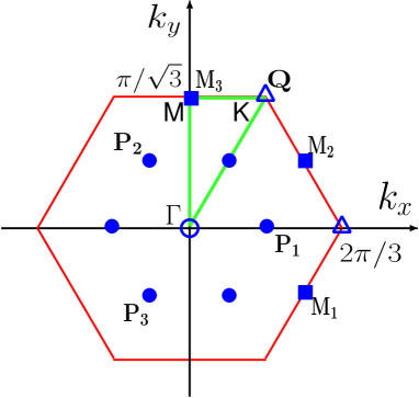
Figure 4: Summary of the main characterizations of the kagome AVL phase. The low-energy excitations are located at wavevectors ${\bf 0}$, $\pm{\bf Q}$, ${\bf M}_{1,2,3}$, and $\pm{\bf P}_{1,2,3}$ in the physical Brillouin zone of the kagome lattice, where ${\bf Q}=(\pi/3,\pi/\sqrt{3})$; ${\bf M}_{1}=(\pi/2,-\pi/(2\sqrt{3}))$, ${\bf M}_{2}=(\pi/2,\pi/(2\sqrt{3}))$, ${\bf M}_{3}=(0,\pi/\sqrt{3})$; ${\bf P}_{1}=(\pi/3,0)$, ${\bf P}_{2}=(-\pi/6,\pi/(2\sqrt{3}))$, and ${\bf P}_{3}=(-\pi/6,-\pi/(2\sqrt{3}))$. Both $S^{z}$ and $S^{+}$ exhibit power law correlations at all these momenta, Eqs. (19) and (22). The $S^{z}$ correlations are “enhanced” ($\eta_{z}\approx 2.46$) for the subset $\pm{\bf Q}$, $\pm{\bf P}_{1,2,3}$ and not enhanced ($\eta_{z}=3$) for the remaining wavevectors. On the other hand, all $S^{+}$ correlations are characterized by the same exponent $\eta_{\pm}\approx 3.24$.

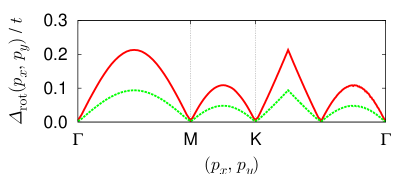
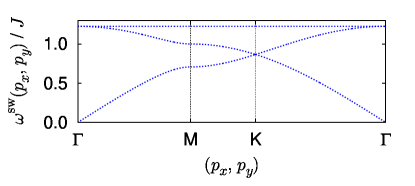
Figure 5: (Top) Lower edge of the vortex-antivortex continuum along several cuts in the Brillouin zone as shown in Fig. 4 for parameter values $t^{\prime}/t=0.5$ and $t^{\prime}/t=0.2$ from the higher to lower curve. (Bottom) Spin wave excitations, Eq. (IV.1), of the kagome XY antiferromagnet with the nearest-neighbour exchange $J$ only along the same cuts in the Brillouin zone.

IV.2 $S^{z}S^{z}$ correlator

A more formal approach towards characterizing the system with gauge interactions is to deduce the PSG transformations for a particular mean-field state.Wen02 Specifically, the notion of symmetry is enlarged to also include gauge transformations in order to maintain invariance of the mean-field Hamiltonian under the usual symmetry operations.

Some details are presented in Appendix C, where we show the calculated transformation properties of the continuum fermion fields $\bar{\psi},\psi$. In particular, with the PSG analysis, the low-energy roton excitations can be studied by analyzing fermion bilinears.

The $S^{z}$-component of the spin is expressed as a gauge flux in our QED₃ theory of vortices. Both the flux induced by the dynamical U(1) gauge field itself and the flux induced by vortex currents contribute to the $S^{z}S^{z}$ correlation. Formally, the $S^{z}$ operator can be expressed in terms of the gauge flux and appropriate fermion bilinears $\bar{\psi}{\cal G}\psi$ representing the contributions by vortex currents,

$$S^{z}_{\mathbf{r}} \sim \frac{\nabla\times\bm{a}}{2\pi}+\sum_{i}A_{i}e^{-i\mathbf{K}_{i}\cdot\mathbf{r}}\bar{\psi}{\cal G}_{i}\psi+\cdots$$ (18)

where the summation over $i$ runs over bilinears $\bar{\psi}{\cal G}_{i}\psi$ with appropriate symmetry properties so that the right hand side transforms identically to $S^{z}$. The factor $e^{-i\mathbf{K}_{i}\cdot\mathbf{r}}$ represents the momenta carried by these bilinears, which are the same as the roton minima shown in Fig. 4, and $A_{i}$ is some amplitude for the bilinear ${\cal G}_{i}$ [in fact, one needs to specify four such amplitudes $A_{i}(j)$ since there are four sites $j=1,\ldots,4$ in the unit cell, Fig. 1].

Assuming the $N=8$ QED₃ is critical, all correlation functions decay algebraically. We then expect to find power law correlation at all momenta shown in Fig. 4. As a consequence, the singular part of the structure factor at zero temperature near such wavevector ${\bf K}$ is given by

$$S^{zz}(\mathbf{k}=\mathbf{K}+\mathbf{q},\omega)\propto\frac{\Theta(\omega^{2}-\mathbf{q}^{2})}{(\omega^{2}-\mathbf{q}^{2})^{(2-\eta_{z})/2}}.$$ (19)

The exponent $\eta_{z}$ characterizes the strength of the $S^{z}$ correlations, and smaller values correspond to more singular and therefore more pronounced correlations. In QED₃, the corresponding exponent value for the flux $\nabla\times a$ that contributes to the $S^{z}$ correlation near zero momentum is $\eta_{z}=3$, and the same exponent also characterizes fermionic bilinears that are conserved currents, see Appendix C. On the other hand, bilinears that are not conserved currents have their scaling dimensions enhanced by the gauge field fluctuations as compared with the mean field. Upon analyzing the transformation properties of the fermionic bilinears, we conclude that there are indeed such enhanced contributions to $S^{z}$ near the momenta $\pm{\bf Q}$ and $\pm{\bf P}_{1,2,3}$ (explicit expressions are given in Appendix C). The new exponent can be estimated from the large-$N$ treatments of the QED₃Rantner02 ; Franz03 to be $\eta_{z}\approx 3-128/(3\pi^{2}N)=2.46$ for $N=8$.

IV.3 $S^{+}S^{-}$ correlator

Since $S^{z}\sim(\nabla\times a)/(2\pi)$, the spin raising operator $S^{+}$ in the dual theory is realized as an operator that creates $2\pi$ gauge flux. Following Ref. Alicea05b, , we treat such flux insertion (“monopole insertion”) classically as a change of the background gauge field configuration felt by fermions. By determining quantum numbers carried by the monopole insertion operators, we can find the wavevectors of the dominant $S^{+}$ correlations.

Here we only outline the procedure (for details, see Refs. Alicea05, ; Alicea05b, ). In the presence of $2\pi$ background flux inserted at $\mathbf{x}=0$, each Dirac fermion species $(\alpha)=1\dots 8$ has a quasi-localized zero-energy state near the inserted flux. We will denote the creation operators for such fermionic zero modes by $f^{{\dagger}}_{(\alpha)}$. The corresponding two-component wavefunctions have the form $\varphi(\mathbf{x})\sim\frac{1}{|\mathbf{x}|}\left(\begin{array}[]{c}1\\ 0\end{array}\right)$, which allows us to relate the transformation properties of $f^{{\dagger}}_{(\alpha)}$ to those of the first component of $\psi^{\dagger}_{(\alpha)}$ (the latter are summarized in Appendix B).

The monopole creation operators ${\cal M}^{\dagger}$ are defined by the combination of the flux insertion and the subsequent filling of four out of eight fermionic zero modes in order to ensure gauge neutrality:

$${\cal M}^{{\dagger}}|DS_{0}\rangle=f^{{\dagger}}_{({\alpha})}f^{{\dagger}}_{({\beta})}f^{{\dagger}}_{({\gamma})}f^{{\dagger}}_{({\delta})}|DS_{+}\rangle,$$ (20)

where $|DS_{0}\rangle$ and $|DS_{+}\rangle$ are the Fermi-Dirac sea in the absence and presence of $+2\pi$ flux, respectively. There are total of $70$ distinct such monopoles. The quantum numbers of the monopole operators are then determined by the transformation properties of the operators $f^{{\dagger}}_{(\alpha)}f^{{\dagger}}_{(\beta)}f^{{\dagger}}_{(\gamma)}f^{{\dagger}}_{(\delta)}$ and those of $|DS_{+}\rangle$ relative to $|DS_{0}\rangle$.

Both $|DS_{+}\rangle$ and $|DS_{0}\rangle$ are expected to be eigenstates of the translation operator $T_{\delta\mathbf{r}}$, and we denote the ratio of the eigenvalues as $e^{{i}\mathbf{\Pi}_{\rm offset}\cdot\delta\mathbf{r}}$. On the other hand, we can diagonalize the action of $T_{\delta\mathbf{r}}$ on $f^{{\dagger}}_{(\alpha)}f^{{\dagger}}_{(\beta)}f^{{\dagger}}_{(\gamma)}f^{{\dagger}}_{(\delta)}$ to get a set of eigenvalues $e^{{i}\mathbf{\Pi}_{i}\cdot\delta\mathbf{r}}$, $i=1,\dots,70$. Thus, the momenta of the monopole operators (at zero energy) are determined by $\{\mathbf{\Pi}_{i}\}$ which are offset by the hitherto unknown wavevector $\mathbf{\Pi}_{\rm offset}$. However, once we examine $\{\mathbf{\Pi}_{i}\}$, we find that the offset is in fact uniquely fixed by the requirement that the monopole momenta are distributed in the physical BZ in a way that respects all lattice symmetries.

Monopole momenta determined in this manner are found to be given by the very same wavevectors ${\bf 0}$, $\pm{\bf Q}$, ${\bf M}_{1,2,3}$, and $\pm{\bf P}_{1,2,3}$, as the leading $S^{z}$ correlation (Fig. 4). For the record, we find the following monopole multiplicities given in the parentheses: ${\bf 0}$ (12 monopoles), $\pm{\bf Q}$ (5 each), ${\bf M}_{1,2,3}$ (8 each), and $\pm{\bf P}_{1,2,3}$ (4 each).

The monopole insertions which add $S^{z}=1$ have overlap with the exact lowest energy spin carrying eigenstates in the AVL. At the lowest energies such eigenstates will be centered around the monopole wavevectors in the Brillouin zone, and we expect that they will disperse with an energy growing linearly with small deviations in the momenta. But presumably any local operator that adds spin one will create a linearly dispersing but overdamped “particle” excitation. More formally, we can expand the $S^{+}$ operator in terms of the continuum fields as follows,

$$S^{+}_{\mathbf{r}} \sim \sum_{i}A_{i}e^{{i}\mathbf{\Pi}_{i}\cdot\mathbf{r}}{\cal M}^{{\dagger}}_{i},$$ (21)

where $\mathbf{\Pi}_{i}$ is the momentum of the monopole ${\cal M}_{i}$. The right hand side has correct transformation properties under the translations, but not all of the monopole operators contribute to $S^{+}$ when other symmetries are taken into account. For example, some of the zero momentum monopoles have opposite eigenvalues under the lattice inversion, and the same happens for the momenta ${\bf M}_{1,2,3}$. However, given the large monopole multiplicities, it appears very likely that all momenta shown in Fig. 4 will be present in $S^{+}$ (but we have not performed an analysis of all quantum numbers so far).

The in-plane dynamical structure factor $S^{+-}$ around each ${\bf\Pi}_{i}$ is thus expected to have the same critical form as $S^{zz}$,

$$S^{+-}(\mathbf{k}=\mathbf{\Pi}+\mathbf{q},\omega)\propto\frac{\Theta(\omega^{2}-\mathbf{q}^{2})}{(\omega^{2}-\mathbf{q}^{2})^{(2-\eta_{\mathrm{\pm}})/2}}~{},$$ (22)

but the characteristic exponent $\eta_{\pm}$ is now that appropriate for the monopole operators and is expected to be the same for all momenta. Ref. Borokhov02, calculated this in the large-$N$ QED₃: $\eta_{\mathrm{mon}}\approx 0.53N-1$. Setting $N=8$, we estimate $\eta_{\mathrm{\pm}}\approx 3.24$, which is larger than even the non-enhanced exponent $\eta_{z}=3$ entering the $S^{z}$ correlations.

The above results with $\eta_{\pm}>\eta_{z}$ suggest that within the AVL phase the system is “closer” to an Ising ordering of $S^{z}$ than of an in-plane XY ordering of $S^{+}$ . This is rather puzzling for an easy-plane spin model, where one would expect XY order to develop more readily than Ising order. This conclusion is reminiscent of the classical kagome spin model, where the easy-plane anisotropy present in the XY model destroys the zero temperature coplanar order of the Heisenberg model. However, this interpretation of the inequality $\eta_{\pm}>\eta_{z}$ is perhaps somewhat misleading. Indeed, as we discuss in Appendix C, condensation of any of the enhanced fermionic bilinears that contribute to $S^{z}$ would drive XY order in addition to $S^{z}$ order - forming a supersolid phase of the bosonic spins. Thus, care must be taken when translating the long-distance behavior of the AVL correlators into ordering tendencies.

The exact diagonalization study by SindzingreSindzingre finds that in the nearest-neighbor kagome XY antiferromagnet the $S^{+}$ correlations are larger than the $S^{z}$ correlations, which is different from the AVL prediction. It would be interesting to examine this further, perhaps also in a model with further-neighbor exchanges. With regards to such numerical studies, we also want to point out that the discussed dynamical spin structure factor, Eqs. (19) and (22), translate into equal-time spin correlations that decay as $r^{-1-\eta_{z,\pm}}$. For the estimated values of $\eta_{z,\pm}$, the decay is rather quick, and could be hard to distinguish from short-range correlations.

V Conclusion

Using fermionized vortices, we have studied the easy-plane spin-1/2 Heisenberg antiferromagnet on the kagome lattice and accessed a novel gapless spin liquid phase. The effective field theory for the resulting Algebraic Vortex Liquid phase, is (2+1)D QED₃ with an emergent $\mathrm{SU}(8)$ flavor symmetry. This large number of flavors can be thought to have its origin in many competing ordered states that are intrinsic to the “loose” network of the corner-sharing triangles in the kagome lattice. It is also likely that for this number of Dirac fermions the critical QED₃ theory is stable against the dynamical gap formation, which allows us to expect that the AVL phase is stable.

The gapless nature of the AVL phase has important thermodynamic consequences. For example, we predict the specific heat to behave as $C\sim T^{2}$ at low temperatures. Since vortices carry no spin, we expect this contribution to be unaffected by the application of a magnetic field. Interestingly, such behavior was observed in SrCr_8-xGa_4+xO₁₉ and was interpreted in terms of singlets dominating the many-body spectrum.Ramirez00 ; Sindzingre00 Since the vortices are mobile and carry energy, we furthermore predict significant thermal conductivity, which would be interesting to measure in such candidate gapless spin liquids.

The more detailed properties of the kagome AVL phase were studied by the PSG analysis, leading to detailed predictions for the spin structure factor. We found that the dominant low energy spin correlations occur at twelve specific locations in the BZ shown in Fig. 4. These wavevectors encode important intermediate-scale physics and can be looked for in experiments and numerical studies. They may be also used to compare and contrast with other theoretical proposals of spin liquid states.

The recent experimentsHelton06 ; Ofer06 ; Mendels06 for the spin-1/2 kagome material ZnCu₃(OH)₆Cl₂ observed power-law behavior in $\omega$ of the structure factor $S(\mathbf{k},\omega)$ in a powder sample. The specific heat measurements and local magnetic probes also suggest gapless spin liquid physics in this compound. Unfortunately, no detailed momentum-resolved information is available so far. It should be also noted that our results were derived assuming easy-plane character of the spin interactions, and do not apply directly if the material has no significant such spin anisotropy. remark 2 Hopefully, more experiments in the near future will provide detailed microscopic characterization of this material, such as the presence/absence of the Dzyaloshinskii-Moriya interaction Rigol07 , and clarify the appropriate spin modeling. In the case of the Heisenberg spin symmetry and nearest-neighbor exchanges, Refs. Hastings01, ; Ran06, offer another candidate critical spin liquid for the kagome lattice, obtained using a slave fermion construction. This algebraic spin liquid (ASL) state differs significantly from the presented AVL phase as discussed in some detail at the end of the introduction and towards the end of Sec. IV.1. Briefly, within the ASL the momentum space locations of the gapless spin carrying excitations are only a small subset of those predicted for the AVL. Moreover, while both phases support gapless Dirac fermions that contribute a $T^{2}$ specific heat, in the AVL phase the fermions (vortices) are spinless in contrast to the fermionic spinons in the ASL. Thus, one would expect the specific heat to be more sensitive to an applied magnetic field in the ASL than in the AVL.

Contrary to SrCr_8-xGa_4+xO₁₉, the experimental data on ZnCu₃(OH)₆Cl₂ shows that the specific heat is affected by the magnetic field in the low temperature regime Helton06 . However, as pointed out by Ran  et al.,Ran06 $T\sim 10\mathrm{K}$ is likely to be an appropriate temperature scale to test several theoretical approaches to this material, since spin liquid physics might be masked by, for example, impurity effects, Dzyaloshinskii-Moriya coupling, or other complicating spin interactions, at the lowest temperature scales. (Indeed, the susceptibility data are perhaps consistent with the presence of impurities, although it is unclear at this stage if the peculiar temperature dependence of the specific heat also has its origins in impurities.) The theoretical prediction of the $T^{2}$ specific heat is consistent with the experiments for $T>10\mathrm{K}$.

A general outstanding issue is the connection, if any, between the critical spin liquids obtained with slave fermions and with fermionic vortices. Perhaps our AVL phase corresponds to some algebraic spin liquid ansatz, but at the moment this is unclear.

Appendix A Zero mode wave functions at the Fermi points

In this appendix, the 16-component wavefunctions $\phi^{\ }_{i,\alpha,a}(n)$ ($n=1,\ldots,16$) representing zero modes at the Fermi points are presented explicitly. These wave functions are necessary for the PSG analysis.

At the node $\mathbf{Q}_{1}$,

$$\phi^{\ }_{\mathrm{I},1,1} = e^{{i}\pi/4}\left(\begin{array}[]{c}\chi^{\mathbf{Q}_{1}}_{A+}\\ 0\end{array}\right),\quad\phi^{\ }_{\mathrm{I},1,2}=e^{{i}\pi/12}\left(\begin{array}[]{c}\chi^{\mathbf{Q}_{1}}_{A-}\\ 0\end{array}\right),\quad$$ (27)

$$\phi^{\ }_{\mathrm{II},1,1} = e^{-{i}\pi/4}\left(\begin{array}[]{c}0\\ \chi^{\mathbf{Q}_{1}}_{B+}\end{array}\right),\,\phi^{\ }_{\mathrm{II},1,2}=e^{-{i}\pi/12}\left(\begin{array}[]{c}0\\ \chi^{\mathbf{Q}_{1}}_{B-}\end{array}\right)~{};$$ (32)

at the node $\mathbf{Q}_{2}$,

$$\phi^{\ }_{\mathrm{I},2,1} = \left(\begin{array}[]{c}\chi_{A+}^{\mathbf{Q}_{2}}\\ 0\end{array}\right),\quad\phi^{\ }_{\mathrm{I},2,2}=e^{{i}\pi/6}\left(\begin{array}[]{c}\chi_{A-}^{\mathbf{Q}_{2}}\\ 0\end{array}\right),$$ (38)

$$\phi^{\ }_{\mathrm{II},2,1} = \left(\begin{array}[]{c}0\\ \chi_{B-}^{\mathbf{Q}_{2}}\end{array}\right),\quad\phi^{\ }_{\mathrm{II},2,2}=e^{-{i}\pi/6}\left(\begin{array}[]{c}0\\ \chi_{B+}^{\mathbf{Q}_{2}}\end{array}\right);$$ (43)

at the node $\mathbf{Q}_{3}$,

$$\phi^{\ }_{\mathrm{I},3,1} = e^{{i}5\pi/4}\left(\begin{array}[]{c}0\\ \chi_{B-}^{\mathbf{Q}_{3}}\end{array}\right),\quad\phi^{\ }_{\mathrm{I},3,2}=e^{{i}13\pi/12}\left(\begin{array}[]{c}0\\ \chi_{B+}^{\mathbf{Q}_{3}}\end{array}\right),$$ (49)

$$\phi^{\ }_{\mathrm{II},3,1} = e^{-{i}\pi/4}\left(\begin{array}[]{c}\chi_{A+}^{\mathbf{Q}_{3}}\\ 0\end{array}\right),\,\phi^{\ }_{\mathrm{II},3,2}=e^{-{i}\pi/12}\left(\begin{array}[]{c}\chi_{A-}^{\mathbf{Q}_{3}}\\ 0\end{array}\right);$$ (54)

and at the node $\mathbf{Q}_{4}$,

$$\phi^{\ }_{\mathrm{I},4,1} = -\left(\begin{array}[]{c}0\\ \chi_{B+}^{\mathbf{Q}_{4}}\end{array}\right),\quad\phi^{\ }_{\mathrm{I},4,2}=e^{{i}7\pi/6}\left(\begin{array}[]{c}0\\ \chi_{B-}^{\mathbf{Q}_{4}}\end{array}\right),\quad$$ (60)

$$\phi^{\ }_{\mathrm{II},4,1} = \left(\begin{array}[]{c}\chi_{A+}^{\mathbf{Q}_{4}}\\ 0\end{array}\right),\quad\phi^{\ }_{\mathrm{II},4,2}=e^{-{i}\pi/6}\left(\begin{array}[]{c}\chi_{A-}^{\mathbf{Q}_{4}}\\ 0\end{array}\right);$$ (65)

where a convenient choice for the eight-component zero energy wave functions $\chi_{A}$ and $\chi_{B}$ is

$$\chi_{A,s}^{\mathbf{Q}_{\alpha}}=N_{A}\left(\begin{array}[]{c}1\\ \alpha\\ (xy)^{2}(y^{4}+(xy^{*})^{2})\\ -\alpha(xy)^{2}(y^{4}-(xy^{*})^{2})\\ -xy^{*3}+\alpha xy^{*}(y^{4}-(xy^{*})^{2})\\ t^{\prime}\left[x^{*}y^{*3}+\alpha xy^{*3}\right]\\ -x^{3}y^{*}\left(y^{4}+(xy^{*})^{2}\right)-\alpha x^{*}y^{*3}\\ t^{\prime}x^{3}y^{*}\left[y^{4}x^{*2}+y^{*2}-\alpha\left(y^{4}-(xy^{*})^{2}\right)\right]\end{array}\right),$$ (67)

$$\chi_{B,s}^{\mathbf{Q}_{\alpha}}=N_{B}\left(\begin{array}[]{c}1\\ \beta\\ (x^{*}y^{*})^{2}(y^{*4}+(x^{*}y)^{2})\\ -\beta(x^{*}y^{*})^{2}(y^{*4}-(x^{*}y)^{2})\\ -t^{\prime}\left[x^{*}y^{3}+\beta xy^{3}\right]\\ x^{*}y\left(y^{*4}+(x^{*}y)^{2}\right)+\beta x^{*}y^{3}\\ t^{\prime}x^{*3}y\left[\beta\left(y^{*4}x^{2}-y^{2}\right)-y^{*4}-(x^{*}y)^{2}\right]\\ xy^{3}-\beta x^{*3}y\left(y^{*4}-(x^{*}y)^{2}\right)\end{array}\right).$$ (68)

Here $x:=e^{{i}k_{x}/2}$, $y:=e^{{i}k_{y}/(2\sqrt{3})}$ for ${\bf Q}=(k_{x},k_{y})$,

$$\alpha = \frac{s3\sqrt{2}x^{*3}y^{*3}-(1+x^{6}y^{6})(x^{4}+x^{*4})}{2x^{-2}(3-x^{2}y^{*6}-x^{*2}y^{6})},$$

$$\beta = \frac{s{i}3\sqrt{2}x^{*3}y^{*3}-(1-x^{6}y^{6})(x^{4}+x^{*4})}{2x^{-2}(3-x^{2}y^{*6}-x^{*2}y^{6})},$$ (69)

and $N_{A}$ and $N_{B}$ are $t^{\prime}$-dependent normalization factors. These zero modes are chosen in such a way that the $s=\pm 1$ wavefunctions are orthogonal to each other for any $t^{\prime}$.

In order to work with the continuum Dirac fields Eq. (12), it is convenient to introduce four sets of the Pauli matrices which act on different gradings. In the following, Pauli matrices denoted by $\rho^{\kappa}$ ($\kappa=0,1,2,3$) act on Latin indices $a=1,2$ ($\rho^{0}$ is an identity matrix). Pauli matrices denoted by $\sigma^{\kappa}$ (and hence $\gamma^{\kappa}$ introduced in Eq. 13) act on Latin indices $i=\mathrm{I},\mathrm{II}$. We separate the node momenta into two groups $(\mathbf{Q}_{1},\mathbf{Q}_{3})$ and $(\mathbf{Q}_{2},\mathbf{Q}_{4})$. Then, Pauli matrices denoted by $\tau^{\kappa}$ act within a given group, either $(\mathbf{Q}_{1},\mathbf{Q}_{3})$ or $(\mathbf{Q}_{2},\mathbf{Q}_{4})$. Finally, Pauli matrices denoted by $\mu^{\kappa}$ act on the space spanned by $(\mathbf{Q}_{1,3},\mathbf{Q}_{2,4})$. We will also use the notation $\tau^{\pm}=\tau^{1}\pm i\tau^{2}$.

Appendix B Projective symmetry group (PSG) analysis

Any symmetry of the original lattice spin model has a representation in terms of vortices. Unfortunately, upon fermionization, time-reversal symmetry transformation becomes highly non-local and we do not know how to implement it in the low-energy effective field theory.

Since a specific configuration of the Chern-Simons gauge field was picked in the flux smearing mean field, we had to fix the gauge and work with the enlarged unit cell. The spatial symmetries of the original lattice spin model are, however, still maintained if the symmetry transformations are followed by subsequent gauge transformations – the original symmetries become “projective symmetries” in the effective field theory. The PSG analysis is necessary when we try to make a connection between the original spin model and the effective field theory.

The original spin system has the following symmetries besides the global $\mathrm{U}(1)$:

$$T_{\mathbf{E}_{1}/2}:\quad\mbox{translation by $\mathbf{E}_{1}/2$},$$

$$T_{\mathbf{E}_{2}}:\quad\mbox{translation by $\mathbf{E}_{2}$},$$

$$R_{\pi}:\quad\mbox{rotation by $\pi$ around a kagome site},$$

$$\mathcal{R}_{x}:\quad\mbox{reflection with respect to $y$ axis},$$

$$\mathcal{C}:\quad\mbox{particle-hole},$$

$$\mathcal{T}:\quad\mbox{time-reversal}.$$ (70)

We can also include a rotation by $\pi/3$ about honeycomb center but will not consider it here.

The first four transformations $T_{\delta\mathbf{r}}$, $R_{\theta}$, $\mathcal{R}_{x}$ act on spatial coordinates $\mathbf{r}=(x,y)$, $\mathbf{r}\to\mathbf{r}+\delta\mathbf{r}$, $\mathbf{r}\to(x\cos\theta-y\sin\theta,x\sin\theta+y\cos\theta)$, $\mathbf{r}\to(-x,y)$, respectively. On the other hand, the particle-hole symmetry $\mathcal{C}$ and the time reversal $\mathcal{T}$ act on spin operators as

$$\mathcal{C}: S^{z}\to-S^{z},\quad S^{x}\pm{i}S^{y}\to S^{x}\mp{i}S^{y},$$

$$\mathcal{T}: \mathbf{S}\to-\mathbf{S},\quad{i}\to-{i}.$$ (71)

Here, the anti-unitary nature of the time reversal is reflected in its action on the complex number ${i}\to-{i}$.

Symmetries in terms of the rotor representation can then be deduced as

$$\mathcal{C}: n\to-n,\quad\varphi\to-\varphi,$$

$$\mathcal{T}: n\to-n,\quad\varphi\to\varphi+\pi,\quad{i}\to-{i}.$$ (72)

Symmetry properties of bosonic and fermionic vortices are deduced from their defining relations. Due to the Chern-Simons flux attachment, the mirror and time-reversal symmetries are implemented in a non-local fashion in the fermionized theory. However, if we combine $\mathcal{T}$ with $\mathcal{R}_{x}$ and $\mathcal{C}$, the resulting modified reflection $\tilde{\mathcal{R}}_{x}:=\mathcal{R}_{x}\mathcal{C}\mathcal{T}$ can still be realized locally. We summarize the symmetry properties of the fermions $d,d^{{\dagger}}$ in Table 1. We also introduce a formal fermion time reversal by

$$\mathcal{T}_{\mathrm{ferm}}:\quad d\to d,\quad{i}\to-{i}.$$ (73)

The necessary explanations are the same as in Refs. Alicea05, ; Alicea05b, and are not repeated here.

	spin $\mathbf{S}$	rotor $\varphi$, $n$
$\mathcal{C}$	$S^{y}\to-S^{y}$, $S^{z}\to-S^{z}$	$n\to-n$, $\varphi\to-\varphi$
$\mathcal{T}$	$\mathbf{S}\to-\mathbf{S}$, ${i}\to-{i}$	$n\to-n$, $\varphi\to\varphi+\pi$, ${i}\to-{i}$
$\tilde{\mathcal{R}}_{x}$	$S^{x}\to-S^{x}$, ${i}\to-{i}$, $x\to-x$	$n\to+n$, $\varphi\to-\varphi+\pi$, ${i}\to-{i}$, $x\to-x$

	vortex $\theta$,$N$ and gauge field $a$, $e$	fermion $d,d^{{\dagger}}$
$\mathcal{C}$	$a\to-a$, $\theta\to-\theta$, $e\to-e$, $N\to 1-N$	$d\to(-1)^{i}d^{\dagger}$
$\mathcal{T}$	$a\to-a$, $\theta\to-\theta$, $e\to e$, $N\to N$, ${i}\to-{i}$
$\tilde{\mathcal{R}}_{x}$	$a\to-a$, $\theta\to-\theta$, $e\to e$, $N\to N$, ${i}\to-{i}$, $x\to-x$	$d\to d$, $x\to-x$, ${i}\to-{i}$

Table 1: Summary of symmetry transformations for spin, rotor, vortex, and fermionized vortex operators on the lattice. The sign factor $(-1)^{i}$ in the action of the particle-hole transformation on the fermionized vortices, $\mathcal{C}:d\to(-1)^{i}d^{\dagger}$, is $1$ on one of the sublattice of the dual lattice whereas it is $-1$ on the other.

Finally, the symmetry properties of the slowly varying continuum fields $\bar{\psi},\psi$ can be deduced from Eq. (12). As explained, these are realized projectively,Wen02 and the symmetry transformations for the continuum fermion fields are summarized in Table 2.

	$T_{\mathbf{E}_{1}/2}$	$T_{\mathbf{E}_{2}}$	$\tilde{\mathcal{R}}_{x}$	$R_{\pi}$	$\mathcal{C}$	$\mathcal{T}_{\mathrm{fermi}}$
$\psi\quad\to\hphantom{AA}$	$\mu^{2}e^{-{i}\pi\tau^{3}/3}\rho^{1}\psi$	$\mu^{3}e^{{i}\pi\tau^{3}/6}\psi$	$e^{+{i}\pi\tau^{3}/12}\tau^{3}e^{+{i}\pi\mu^{2}\rho^{1}/4}\rho^{3}\psi$	$\sigma^{3}\rho^{2}\tau^{1}e^{{i}5\pi\tau^{3}/12}\mu^{3}\psi$	$\tau^{1}\sigma^{1}\left[\psi^{{\dagger}}\right]^{T}$	$\tau^{2}\sigma^{2}\psi$

Table 2: Summary of symmetry transformations for continuum fermion fields (upto unimportant $\mathrm{U}(1)$ phase factors).

Appendix C Fermion bilinears

Once we determine the symmetry properties of the continuum fermion fields $\bar{\psi},\psi$, we can discuss symmetry properties of the gauge invariant bilinears $\bar{\psi}\mathcal{G}\psi$ where $\mathcal{G}$ is a $16\times 16$ matrix. Using the gradings specified at the end of Appendix A, the bilinears can be conveniently written as

$$\bar{\psi}\sigma^{\kappa}\mu^{\lambda}\tau^{\alpha}\rho^{\beta}\psi$$ (74)

where $\kappa,\lambda,\alpha,\beta$ run from $0$ to $3$ and hence there are $4^{4}=64\times 4$ such bilinears. Among these bilinears, $64\times 3$ bilinears with the Lorentz index $\kappa=1,2,3$ represent $\mathrm{U}(8)$ currents,

$$\bar{\psi}\sigma^{1,2,3}\mu^{\lambda}\tau^{\alpha}\rho^{\beta}\psi.$$ (75)

On the other hand, there are $64$ remaining bilinears with $\kappa=0$,

$$\bar{\psi}\sigma^{0}\mu^{\lambda}\tau^{\alpha}\rho^{\beta}\psi.$$ (76)

Since the bilinears (75) are conserved currents, they maintain their engineering scaling dimensions even in the presence of the gauge fluctuations. On the other hand, the bilinears of the form (76) (“enhanced bilinears”) develop anomalous dimensions when we include the gauge fluctuations.

Let us give some relevant examples of bilinears. The $\sqrt{3}\times\sqrt{3}$ magnetically ordered state (shown in Fig. 1) corresponds to the staggered charge density wave of vortices, which is obtained by adding the corresponding staggered chemical potential (i.e., $\pm\delta\mu$ on the up/down kagome triangles). Using the listed symmetries, it is readily verified that the following two bilinears in the expression

$$B_{\sqrt{3}\times\sqrt{3}}=\alpha\;\bar{\psi}\sigma^{0}\mu^{0}\tau^{3}\rho^{0}\psi+\beta\;\bar{\psi}\sigma^{3}\mu^{3}\tau^{0}\rho^{3}\psi$$ (77)

transform in the manner expected of the staggered chemical potential (the coefficients $\alpha$ and $\beta$ are generically independent). This can be also checked explicitly by writing such chemical potential in terms of the continuum fields obtaining some $t^{\prime}$-dependent coefficients $\alpha$ and $\beta$. In the similar vein, the $q=0$ state (also shown in Fig. 1) corresponds to the uniform chemical potential for vortices on the up and down kagome triangles, which is realized with the following bilinears

$$B_{q=0}=\alpha^{\prime}\;\bar{\psi}\sigma^{0}\mu^{3}\tau^{3}\rho^{3}\psi+\beta^{\prime}\;\bar{\psi}\sigma^{3}\mu^{0}\tau^{0}\rho^{0}\psi~{}.$$ (78)

Note that each $B_{\sqrt{3}\times\sqrt{3}}$ and $B_{q=0}$ contains an enhanced bilinear of the QED₃ theory, and therefore both orders are “present” in the AVL phase as enhanced critical fluctuations. It is in such sense that the enhanced bilinears encode the potential nearby orders.

With the table 2 at hand, it is a simple matter to check that spatial symmetries (translation, rotations, and reflection) and particle-hole symmetry prohibit all fermion bilinears from appearing in the effective action (15), except $\bar{\psi}\psi$ and $\bar{\psi}\sigma^{3}\mu^{3}\tau^{3}\rho^{3}\psi$. If we are allowed to require the invariance under $\mathcal{T}_{\mathrm{ferm}}$, then these bilinears would be prohibited as well. However, even if we do not use $\mathcal{T}_{\mathrm{ferm}}$, we exclude these bilinears from the continuum theory using the following argument from Ref. Alicea05b, : Consider first adding the bilinear $\bar{\psi}\psi$ to the action and analyze the resulting phase for the original spin model. This bilinear opens a gap in the fermion spectrum, and proceeding as in Ref. Alicea05b, we conclude that this phase is in fact a chiral spin liquid that breaks the physical time reversal. Therefore, if we are interested in a time-reversal invariant spin liquid, we are to exclude this term. The situation with the $\bar{\psi}\sigma^{3}\mu^{3}\tau^{3}\rho^{3}\psi$ term is less clear since by itself it would lead to small Fermi pockets, and it is then difficult to deduce the physical state of the original spin system. In the presence of both terms, depending on their relative magnitude one may have either a gap or Fermi pockets. However, we can plausibly argue that these pockets tend to be unstable towards a gapped phase that is continuously connected to the same chiral phase obtained when the mass term $\bar{\psi}\psi$ dominates. Since we are primarily interested in the states that are not chiral spin liquid (e.g., states that appear from the AVL description by spontaneously generating some other mass terms like $B_{\sqrt{3}\times\sqrt{3}}$ or $B_{q=0}$), we drop the bilinears $\bar{\psi}\psi$ and $\bar{\psi}\sigma^{3}\mu^{3}\tau^{3}\rho^{3}\psi$ from further considerations. The validity of this assumption and the closely related issue of neglecting irrelevant higher-derivative Chern-Simons terms from the final AVL action are the main unresolved questions about the AVL approach (see Ref. Alicea05b, for some discussion).

As another example of the application of the derived PSG, we write explicitly combinations of enhanced bilinears that contribute to $S_{j}^{z}\sim(\nabla\times a)_{j}/(2\pi)+G_{j}+F_{j}+\dots$:

$$G_{j} = g_{j}\left(e^{i{\bf Q}\cdot{\bf r}_{j}}e^{-i{\pi}/{12}}B_{Q}^{+}+{\rm h.c.}\right)~{},$$ (79)

$$F_{j} = f^{1}_{j}\left(e^{i{\bf P}_{1}\cdot{\bf r}_{j}}e^{i{5\pi}/{12}}B_{P_{1}}^{+}+{\rm h.c.}\right)$$ (80)

$$+f^{2}_{j}\left(e^{i{\bf P}_{2}\cdot{\bf r}_{j}}e^{i{5\pi}/{12}}B_{P_{2}}^{+}+{\rm h.c.}\right)$$

$$+f^{3}_{j}\left(e^{i{\bf P}_{3}\cdot{\bf r}_{j}}e^{i{5\pi}/{12}}B_{P_{3}}^{+}+{\rm h.c.}\right)~{}.$$

Here $j$ refers to the “basis” labels in the unit cell consisting of four sites in the extended model shown in Fig. 1; the wave vectors are the ones shown in Fig. 4, while the corresponding bilinears are $B_{Q}^{+}=\bar{\psi}\mu^{2}\tau^{+}\rho^{0}\psi$, $B_{P_{1}}^{+}=\bar{\psi}\mu^{3}\tau^{+}\rho^{2}\psi$, $B_{P_{2}}^{+}=\bar{\psi}\mu^{2}\tau^{+}\rho^{3}\psi$, $B_{P_{3}}^{+}=\bar{\psi}\mu^{0}\tau^{+}\rho^{2}\psi$. The above is to be interpreted as an expansion of the microscopic operators $S_{j}^{z}$ defined on the original spin lattice sites in terms of the continuum fields in the theory. It is straightforward but tedious to verify that one can choose real parameters $g_{j}$ and $f^{1,2,3}_{j}$ so that $G$ and $F$ have identical transformation properties with $\nabla\times a$ and therefore indeed contribute to $S^{z}$. We thus conclude that $S^{z}$ has enhanced correlations at the wavevectors $\pm{\bf Q}$, $\pm{\bf P}_{1,2,3}$ as claimed in the main body.

References

- (1) D. A. Huse and A. D. Rutenberg, Phys. Rev. B 45, 7536 (1992).
- (2) C. Zeng and V. Elser, Phys. Rev. B 42, 8436 (1990).
- (3) R. R. P. Singh and D. A. Huse, Phys. Rev. Lett. 68, 1766 (1992).
- (4) P. W. Leung and V. Elser, Phys. Rev. B 47, 5459 (1993).
- (5) N. Elstner and A. P. Young, Phys. Rev. B 50, 6871 (1994).
- (6) P. Lecheminant, B. Bernu, C. L’huillier, L. Pierre, and P. Sindzingre, Phys. Rev. B 56, 2521 (1997).
- (7) Ch. Waldtmann, H.-U. Everts, B. Bernu, C. Lhuillier, P. Sindzingre, P. Lecheminant, and L. Pierre, Eur. Phys. J. B 2, 501 (1998)
- (8) P. Sindzingre, G. Misguich, C. Lhuillier, B. Bernu, L. Pierre, Ch. Waldtmann, and H.-U. Everts, Phys. Rev. Lett. 84, 2953 (2000).
- (9) G. Misguich and B. Bernu, Phys. Rev. B 71, 014417 (2005).
- (10) X. Obradors, A. Labarta, A. Isalgue, J. Tejada, J. Rodrituez, and M. Perret, Sol. St. Comm. 65, 189 (1988).
- (11) A. P. Ramirez, G. P. Espinosa, and A. S. Cooper, Phys. Rev. Lett. 64, 2070 (1990).
- (12) C. Broholm, G. Aeppli, G. P. Espinosa, and A. S. Cooper, Phys. Rev. Lett. 65, 3173 (1990).
- (13) A. P. Ramirez, G. P. Espinosa, and A. S. Cooper, Phys. Rev. B 45, 2505 (1992).
- (14) A. P. Ramirez, B. Hessen, and M. Winklemann, Phys. Rev. Lett. 84, 2957 (2000).
- (15) A. S. Wills, Phys. Rev. B 63, 064430 (2001).
- (16) T. Inami, M. Nishiyama, S. Maegawa, and Y. Oka, Phys. Rev. B 61, 12181 (2000).
- (17) S.- H. Lee, C. Broholm, M. F. Collins, L. Heller, A. P. Ramirez, Ch. Kloc, E. Bucher, R. W. Erwin, and N. Lacevic, Phys. Rev. B 56, 8091 (1997).
- (18) Z. Hiroi, M. Hanawa, N. Kobayashi, M. Nohara, H. Takagi, Y. Kato, and M. Takigawa, J. Phys. Soc. Jpn. 70, 3377 (2001).
- (19) J. S. Helton, K. Matan, M. P. Shores, E. A. Nytko, B. M. Bartlett, Y. Yoshida, Y. Takano, Y. Qiu, J. -H. Chung, D. G. Nocera, and Y. S. Lee, cond-mat/0610539.
- (20) O. Ofer, A. Keren, E. A. Nytko, M. P. Shores, B. M. Bartlett, D. G. Norcera, C. Baines, and A. Amato, cond-mat/0610540.
- (21) P. Mendels, F. Bert, M. A. de Vries, A. Olariu, A. Harrison, F. Duc, J. C. Trombe, J. Lord, A. Amato, and C. Baines, cond-mat/0610565.
- (22) R. Masutomi, Y. Karaki, and H. Ishimoto, Phys. Rev. Lett. 92, 025301 (2004).
- (23) V. Elser, Phys. Rev. Lett. 62, 2405 (1989).
- (24) S. Sachdev, Phys. Rev. B 45, 12377 (1992).
- (25) F. Wang and A. Vishwanath, Phys. Rev. B 74, 174423 (2006).
- (26) L. Balents, M.P.A. Fisher and S.M. Girvin, Phys. Rev. B 65, 224412 (2002).
- (27) G. Misguich, D. Serban, and V. Pasquier Phys. Rev. Lett. 89, 137202 (2002).
- (28) K. Yang, L. K. Warman, and S. M. Girvin, Phys. Rev. Lett. 70, 2641 (1993).
- (29) J. B. Marston and C. Zeng, J. Appl. Phys. 69, 5962 (1991).
- (30) M. B. Hastings, Phys. Rev. B 63, 014413 (2001).
- (31) Y. Ran, M. Hermele, P. A. Lee, and X.-G. Wen, cond-mat/0611414.
- (32) J. Alicea, O. I. Motrunich, M. Hermele, and M. P. A. Fisher, Phys. Rev. B 72 064407, (2005).
- (33) J. Alicea, O. I. Motrunich, and M. P. A. Fisher, Phys. Rev. Lett. 95, 247203 (2005).
- (34) J. Alicea, O. I. Motrunich, and M. P. A. Fisher, Phys. Rev. B 73, 174430 (2006).
- (35) P. Sindzingre, unpublished.
- (36) W. Zheng, J. O. Fjaerestad, R. R. P. Singh, R. H. McKenzie, and R. Coldea, Phys. Rev. Lett. 96 057201 (2006).
- (37) W. Zheng, J. O. Fjaerestad, R. R. P. Singh, R. H. McKenzie, and R. Coldea, cond-mat/0608008.
- (38) O. A. Starykh, A. V. Chubukov, and A. G. Abanov, Phys. Rev. B 74, 180403(R) (2006).
- (39) J. Alicea and M. P. A. Fisher, cond-mat/0609439.
- (40) S. J. Hands, J. B. Kogut, and C. G. Strouthos, Nucl. Phys. B 645, 321 (2002).
- (41) S. J. Hands, J. B. Kogut, L. Scorzato, and C. G. Strouthos, Phys. Rev. B 70, 104501 (2004).
- (42) When Dirac fermions and photons are decoupled, both of them give rise to contributions to specific heat due to their relativistic energy spectra. The effect of gauge fluctuations can be studied systematically for large numbers of fermion flavor . (See also discussions in Ref. Ran06, .) One way to see how gauge interactions affect the specific heat is to integrate out fermions and derive the propagator for dressed photons, which becomes . Rantner02 ; Franz03 ; Hermele05 Calculating the free energy of such photons at finite temperature, one can then see that the specific heat still behaves as , although the ”damped” dynamics of photons does modify the proportionality constant.
- (43) W. Rantner and X. -G. Wen, Phys. Rev. B 66, 144501 (2002).
- (44) M. Franz, T. Pereg-Barnea, D. E. Sheehy, and Z. Tesanovic, Phys. Rev. B 68, 024508 (2003).
- (45) M. Hermele, T. Senthil, M. P. A. Fisher, Phys. Rev. B 72, 104404 (2005).
- (46) L. B. Ioffe and G. Kotliar, Phys. Rev. B 42, 10348 (1990).
- (47) P. A. Lee and N. Nagaosa, Phys. Rev. B 46, 5621 (1992).
- (48) The double degeneracy that we find is reminiscent of that in O. Vafek and A. Melikyan, Phys. Rev. Lett. 96, 167005 (2006).
- (49) A. B. Harris, C. Kallin, and A. J. Berlinsky, Phys. Rev. B 45, 2899 (1992).
- (50) A. Chubukov, Phys. Rev. Lett. 69, 832 (1992).
- (51) V. Borokhov, A. Kapustin, and X. Wu, JHEP 0211, 049 (2002).
- (52) For example, Dzyaloshinskii-Moriya interactions can provide the desired easy plane anisotropy. However, typically such interactions also break some lattice symmetries, such as inversions. In terms of our effective field theory approach, they could then modify the set of fermion bilinears allowed by symmetry, which may lead to an instability of the critical spin liquid state we discuss. Nevertheless, there may still be a range of energy scales over which the spin liquid might provide a reasonable description of an experimental system such as herbertsmithite. These issues were addressed in Refs. Alicea05a, ; Alicea05b, that discuss geometrically frustrated quantum magnets on the triangular lattice, motivated by Dzyaloshinskii-Moriya interaction in CsCuCl.
- (53) M. Rigol, and R. P. Singh, cond-mat/0701087.
- (54) X. G. Wen, Phys. Rev. B 65, 165113 (2002); cond-mat/0107071.