Exciting half-integer charges in a quantum point contact

Abstract

We study a voltage-driven quantum point contact (QPC) strongly coupled to a qubit. We predict pronounced observable features in the QPC current that can be interpreted in terms of half-integer charge transfers. Our analysis is based on the Keldysh generating functional approach and contains general results, valid for all coherent conductors.

The quantum point contact vWee88 has become a basic concept in the field of Quantum Transport owing to its simplicity. Its common experimental realization is a narrow constriction that connects two metallic reservoirs. An adequate theoretical description for this setup is a non-interacting one-dimensional electron gas interrupted by a potential barrier. The barrier is completely characterized by its scattering matrix. This enables the scattering approach to Quantum Transport But90 . This allows one to describe the average current through the QPC, as well as fluctuations away from this average, in terms of single electrons passing through the constriction Lev96 . The strength of the scattering approach is its ability to describe not only traditional realizations of a QPC, but all coherent conductors, including diffusive wires and tunneling junctions.

Despite the correctness of the non-interacting electron description, truly many-body quantum correlations do exist and are observable in a QPC. They manifest themselves in the full counting statistics of electron transfers Lev96 and allow for detection of two-particle entanglement Been03 through the measurement of non-local current correlations. This suggests that the observation of many-body effects in a QPC crucially relies on a proper detection scheme. In this Letter, we give an example of how an appropriate detector uncovers such non-trivial many-body effects as half-integer charges.

We probe the QPC with a charge qubit. Such a device has already been realized using single and double quantum dots. Previously, the QPC has been used as a detector of the qubit state Elz03 ; Pet04 . We propose a scheme in which the roles are reversed. Provided the qubit and QPC are coupled strongly, the switching between the qubit states is accompanied by severe Fermi-Sea shake-up in the QPC. The d.c. current in the QPC is sensitive to the ratio of the qubit switching rates and thereby provides information about these severe shake-ups.

Before analising the system in detail, the following qualitative conclusions can be drawn. The qubit owes its detection capabilities to the following fact: In order to be excited it has to absorb a quantum $\varepsilon$ of energy from the QPC. Here $\varepsilon$ is the qubit level splitting, a parameter that can be tuned easily in an experiment by means of a gate voltage. The QPC supplies the energy by transfering charge from the high voltage reservoir to the low voltage reservoir. The transfer of charge $q$ allows qubit transitions for level splittings $\varepsilon<qV$, $V$ being the bias voltage applied.

We can assume that successive switchings of the qubit between its states $\left|1\right>$ and $\left|2\right>$ are rare and uncorellated. The qubit dynamics are then characterized by the rates $\Gamma_{21}$ to switch from state $\left|1\right>$ to state $\left|2\right>$ and $\Gamma_{12}$ from $\left|2\right>$ to $\left|1\right>$. The stationary probability to find the qubit in state $\left|2\right>$ is determined by detailed balance to be $p_{2}=\Gamma_{21}/(\Gamma_{12}+\Gamma_{21})$. This probability can be observed experimentally by measuring the current in the QPC. The current displays random telegraph noise, switching between two values $I_{1}$ and $I_{2}$. These correspond to the qubit being in the state $\left|1\right>$ or $\left|2\right>$ respectively. The d.c. current $I$ gives the average over many switches and is thus related to the stationary probability by $I=(1-p_{2})I_{1}+p_{2}I_{2}$. The values of $I_{1}$, $I_{2}$ and $I$ are determined through measurement and $p_{2}$ is inferred.

When the QPC and qubit are weakly coupled Ale97 ; Levi97 , a single electron is transfered Onac06 . This liberates at most energy $eV$, implying that the rate $\Gamma_{21}$ is zero when $\varepsilon>eV$ and the rate $\Gamma_{12}$ is zero when $\varepsilon<-eV$. The resulting $p_{2}$ changes from $1$ to $0$ upon increasing $\varepsilon$ within the interval $-eV<\varepsilon<eV$. Cusps at $\varepsilon=\pm eV$ signify that charge $e$ is transferred. [See Fig. (2a)]

Guided by our understanding of weak coupling we can speculate as follows about what happens at strong coupling. Apart from single electron transfers, we also expect the coordinated transfers of groups of electrons. A group of $n$ electrons can provide up to $neV$ of energy to the qubit. Therefore, peculiarities in $p_{2}$ should appear at the corresponding level splittings $\varepsilon=\pm neV$, $n=1,2,3,\ldots$Tob06 However, it is not apriori obvious that these peculiarities are pronounced enough to be observed. The reason is the decoherence of the qubit states induced by electrons passing through the QPC. The Fourier transform of the qubit transition rate acquires an exponential damping factor $e^{-W|t|}$, $W^{-1}$ being the decoherence time. This smoothes out peculiarities at the energy scale $W$. In the strong coupling regime, the decoherence time is estimated to be short, $W\simeq eV/$. As a result, it is not clear whether peculiarities at $neV$ are the dominant feature at strong coupling.

Therefore, strong coupling of the QPC and the qubit requires quantitative analysis. We have reduced the problem to the evaluation of a determinant of an infinite-dimensional Wiener-Hopf operator. We calculated the determinant numerically and found that peculiarities at multiples of $eV$ are minute. Their contribution to $p_{2}$ does not exceed $10^{-4}$ and is seen only at logarithmic scale and at moderate couplings. Instead, far more prominent features occurs at $\varepsilon=\tfrac{1}{2}eV$. General reasoning does not predict this. Straight-forward energy balance arguments force us to conclude that qubit switching is accompanied by the transfer of charge $e/2$ through the QPC. This frees up energy $eV/2$, stimulating qubit transitions when $\varepsilon<eV/2$. In other words, the qubit switching excites a half-integer charge and simultaneously detects it. Fractional charge is known to occur in strongly interacting many-electron systems Lau83 ; Jac76 ; Sut90 in equilibrium. In contrast to this, the electrons in the QPC can be regarded non-interacting except during the short time the qubit is switching. Our system is also unusual in that the half-integer charge is only produced during qubit switching and is not present in the equilibrium state.

Let us now turn to the details of our analysis. The system is illustrated in Fig. (1).

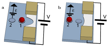
Figure 1: A schematic picture of the system considered. It consists of a charge qubit coupled to a QPC. The shape of the QPC constriction, and hence its scattering matrix, depends on the state of the qubit. The QPC is biased at voltage $V$. A gate voltage controls the qubit level splitting $\varepsilon$. There is a small tunneling rate $\gamma$ between qubit states.

The Hamiltonian for the system is

$$\hat{H}=\hat{T}+\hat{U}_{1}\left|1\right>\left<1\right|+(\hat{U}_{2}+\varepsilon)\left|2\right>\left<2\right|+\gamma(\left|1\right>\left<2\right|+\left|2\right>\left<1\right|)$$ (1)

The operator $\hat{T}$ represents the kinetic energy of QPC electrons. The operator $\hat{U}_{k}$ describes the potential barrier seen by QPC electrons when the qubit is in state $k=1,\ 2$ and corresponds to a scattering matrix $\check{s}_{k}$ in the scattering approach. (We use a “check” to indicate a matrix in the space of transport channels.) QPC electrons do not interact directly with each other but rather with the qubit. This interaction is the only qubit relaxation mechanism included in our model. We work in the limit $\gamma\to 0$ where the inelastic transition rates $\Gamma_{12,21}$ between qubit states are small compared to the energies $eV$ and $\varepsilon$. In this case, the qubit switching events can be regarded as independent and incoherent.

Now consider the qubit transition rate $\Gamma_{21}$. To lowest order in the tunneling amplitude $\gamma$ it is given by

$$\Gamma_{21}= 2\gamma^{2}{\rm Re}\,\int_{-\infty}^{0}d\tau\,e^{i\varepsilon\tau}$$

$$\times\lim_{t_{0}\to-\infty}{\rm tr}\left[e^{i\hat{H}_{2}\tau}e^{-i\hat{H}_{1}(\tau-t_{0})}\rho_{0}e^{i\hat{H}_{1}(\tau-t_{0})}\right].$$ (2)

This is the usual Fermi Golden Rule. The Hamiltonians $\hat{H}_{1}$ and $\hat{H}_{2}$ are given by $\hat{H}_{k}=\hat{T}+\hat{U}_{k}$ and represent QPC dynamics when the qubit is held fixed in state $\left|k\right>$. The trace is over QPC states, and $\rho_{0}$ is the initial QPC density matrix. The evaluation of the integrand is a special case of a general problem in the extended Keldysh formalism Naz03 . The task is to evaluate the trace of a density matrix after “bra’s” have evolved with a time-dependent Hamiltonian $\hat{H}_{-}(t)$ and “kets” with a different Hamiltonian $\hat{H}_{+}(t)$.

$$e^{\mathcal{A}}={\rm tr}\left[\mathcal{T}^{+}e^{-i\int_{-\infty}^{\infty}dt\,\hat{H}_{+}(t)}\rho_{0}\mathcal{T}^{-}e^{i\int_{-\infty}^{\infty}dt\,\hat{H}_{-}(t)}\right].$$ (3)

We implemented the scattering approach to obtain the general formula

$$\mathcal{A}={\rm tr\,ln}\left[\hat{s}_{-}(1-\hat{f})+\hat{s}_{+}\hat{f}\right]-{\rm tr\,ln\,}\hat{s}_{-}.$$ (4)

The operators $\hat{s}_{\pm}$ and $\hat{f}$ have both continuous and discrete indices. The continuous indices refer to energy, or in the Fourier transformed representation, to time. The discrete indices refer to transport channel space. The operators $\hat{s}_{\pm}=\check{s}_{\pm}(t)\delta(t-t^{\prime})$ are diagonal in time. The time-dependent scattering matrices $\check{s}_{\pm}(t)$ describe scattering by the Hamiltonians $\hat{H}_{\pm}(t)$ at instant $t$. (It is the hall-mark of the scattering approach to express quantities in terms of scattering matrices rather than Hamiltonians.) The operator $\hat{f}=\check{f}(E)\delta(E-E^{\prime})$ is diagonal in the energy representation. The matrix $\check{f}(E)$ is diagonal in channel space, representing the individual electron filling factors in the different channels. A full derivation of Eq. (4) will be given elsewhere. It generalizes similar relations published in Aba04 ; Aba05 .

In order to apply the general result to Eq. (2), the time-dependent scattering matrices $\check{s}_{\pm}(t)$ are chosen as

$$\check{s}_{+}(t)= \check{s}_{1}+\theta(t-\tau)\theta(-t)(\check{s}_{2}-\check{s}_{1}),$$ (5)

$$\check{s}_{-}= \check{s}_{1}.$$ (6)

The QPC scattering matrices $\check{s}_{1}(\check{s}_{2})$ with the qubit in the state $1(2)$ are the most important parameters of our approach.

Without a bias-voltage applied, the QPC-qubit setup exhibits the physics of the Anderson orthogonality catastrophe And67 . For the equilibrium QPC, the problem can be mapped Aba04 onto the classic Fermi Edge singularity (FES) problem Mah67 ; Noz69 ; Mat92 . The authors of Aba04 effectively computed $\mathcal{A}$ in equilibrium. Our setup is simpler than the generic FES problem since there is no tunneling from the qubit to the QPC. As a result, not all processes considered in Aba04 are relevant for our setup. We only need the so-called closed loop contribution. The relevant part of the FES result for our setup is an anomalous power law $\Gamma_{21}^{(0)}(\varepsilon)=\theta(-\varepsilon)\frac{1}{|\varepsilon|}\left(\frac{|\varepsilon|}{E_{\rm c.o.}}\right)^{\alpha}$ for the equilibrium rate. Here $E_{\rm c.o.}$ is an upper cutoff energy. The anomalous exponent $\alpha$ is determined by the eigenvalues of $\check{s}_{2}^{\dagger}\check{s}_{1}$ Yam82 as $\alpha=\tfrac{1}{4\pi^{2}}\left|{\rm Tr}\,\ln^{2}(\hat{s}_{f}^{\dagger}\hat{s}_{i})\right|$. The logarithm is defined on the branch $(-\pi,\pi]$. For a one or two channel point contact, $0<\alpha<1$.

We now give the details of our calculation for the rates out of equilibrium. From Eq. (2) and Eq. (4) it follows that $\Gamma_{21}(\varepsilon)\propto|\gamma^{2}|\int_{-\infty}^{\infty}d\tau\ e^{-i\varepsilon\tau}{\rm Det}\ \hat{Q}^{(V)}(\tau)$. For positive times $\tau$, the operator $\hat{Q}^{(V)}(\tau)$ is defined as Aba04 .

$$\hat{Q}^{(V)}(\tau)=1+(\check{s}_{2}^{-1}\check{s}_{1}-1)\hat{\Pi}(\tau)\hat{f}^{(V)}$$ (7)

while for negative $\tau$, $\hat{Q}^{(V)}(\tau)=\hat{Q}^{(V)}(-\tau)^{\dagger}$ The time-interval operator $\hat{\Pi}(\tau)=\delta(t-t^{\prime})\theta(t)\theta(\tau-t)$ is diagonal in time and acts as the identity operator in channel space for times $t=t^{\prime}\in[0,\tau]$ and as the zero-operator outside this time-interval.

For the purpose of numerical calculation of the determinant we have to regularise $\hat{Q}^{(V)}(\tau)$. This is done by multiplying with the inverse of the zero-bias operator to define a new operator $\tilde{Q}(\tau)=\left.\hat{Q}^{(0)}(\tau)\right.^{-1}\hat{Q}^{(V)}(\tau)$. Its determinant is evaluated numerically. The rate $\Gamma_{21}(\epsilon)$ at bias voltage $V$ is then expressed as the convolution $\Gamma_{21}(\varepsilon)=\int\tfrac{d\varepsilon^{\prime}}{2\pi}\Gamma^{\rm eq}_{21}(\varepsilon-\varepsilon^{\prime})\tilde{P}(\varepsilon^{\prime})$ of the equilibrium rate and the Fourier transform of $\tilde{P}(\tau)={\rm Det}\,\tilde{Q}^{(V)}(\tau)$, that contains all effects of the bias voltage $V$.

We implemented this calculation numerically, and computed the probability $p_{2}$ to find the qubit in state $\left|2\right>$. Details of our numerical method are presented in Appendix A. Our main results are presented in Fig. (2).

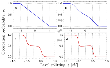
Figure 2: The occupation probability $p_{2}$ of qubit state $\left|2\right>$. At weak coupling between the QPC and qubit, (Fig. a, b) the transfer of a single electron with charge $e$ is detected. Peculiarities at $\pm eV/2$ at strong coupling (Fig. c, d) constitute the detection of half integer charges $e/2$. Scattering matrices were parameterized as in Eq. 8. Fig. a, b, c and d respectively correspond to $\phi=\pi/16$, $\pi/4$, $7\pi/10$ and $4\pi/5$.

We used $2\times 2$ scattering matrices parametrized by

$$\check{s}_{2}^{-1}\check{s}_{1}=\left(\begin{array}[]{cc}\cos\phi&i\sin\phi\\ i\sin\phi&\cos\phi\end{array}\right)$$ (8)

and repeated the calculation for several $\phi\in[0,\pi]$. Small $\phi$ corresponds to weak coupling. The curve at $\phi=\pi/16$ is almost indistinguishable from the perturbative weak coupling limit discussed in the introduction. Cusps at $\pm eV$ indicate that qubit switching is accompanied by the transfer of charge $e$ in the QPC.

The increasing decoherence smoothes the cusps for the curve at $\phi=\pi/4$ (2b). When the coupling is increased beyond $\phi=\pi/2$ steps appear at $\pm eV/2$ (c). This implies charge fractionalization $e\rightarrow e/2$. Further increase of the coupling results in a sharpening of the steps (d).

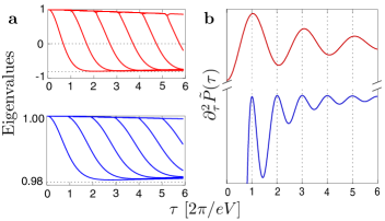
Figure 3: The behavior of eigenvalues for at weak and strong QPC-qubit coupling respectively. The parameter $\phi$ that parameterises the scattering matrix equals $\pi/16$ (bottom) and $4\pi/5$ (top) representing the weak and strong coupling limits respectively. For $\phi=\pi/16$ individual eigenvalues travel from $1$ to $\cos\pi/16\simeq 0.9808$ at a rate of approximately one per $2\pi/eV$. For $\phi=4\pi/5$, eigenvalues travel towards $\cos 4\pi/5\simeq-0.8090<0$ at a rate of one per $2\pi/eV$, as shown in (a). Deviations from the correct asymptotics are due to finite size effects. Figure ($\bf b$) contains the second derivative of $\tilde{P}(\tau)={\rm Det}\ \hat{Q}^{(0)}(\tau)^{-1}\hat{Q}^{(V)}(\tau)$. (The second derivative is taken to remove an average slope and curvature.) Oscillations with period $h/eV$ are seen (bottom) for $\phi=\pi/16$, while for $\phi=4\pi/5$ (top), the periodicity of $\tilde{P}(\tau)$ doubles.

Known mechanisms of charge fractionalization do not seem to provide an immediate explanation of our findings. The Quantum Hall mechanism Lau83 does not give even fractions while the instanton mechanism Jac76 requires a quasiclassical boson field. There is an indirect analogy with the model of interacting particles on a ring threaded by a magnetic flux Sut90 . There, one expects that the energy eigenvalues are periodic in flux with period of one flux quantum. However, the exact Bethe-Ansatz solution Sut90 reveals a double period of eigenvalues with adiabatically varying flux. This is a signature of half-integer charge quantization.

For our non-equilibrium setup, energy eigenvalues are not particulary useful. The natural eigenvalues to describe the phenomenon are those of the oprator $\tilde{Q}^{(V)}(\tau)$. They depend on the parameter $eV\tau$ which is an analogue of flux. The product of the eigenvalues, i.e. the determinant $\tilde{P}(\tau)$ is not precisely periodic in $\tau$ since it decays at large $\tau$ owing to decoherence. Still, it oscillates and the period of these oscillations doubles as we go from weak to strong coupling (Fig. 3b). The doubling can be understood in terms of the transfer of the eigenvalues of $\tilde{Q}^{(V)}(\tau)$ upon increasing $\tau$ (Fig 3a) assuming the parametrization (8). In the large $\tau$ limit, energy-time uncertainty can be neglected in a “quasi-classical” approximation: The operator $\hat{\Pi}(\tau)$ projects onto a very long time interval, and is replaced by the identity operator. $\tilde{Q}^{(V)}$ becomes diagonal in energy. All eigenvalues that are not equal to $1$ are concentrated in the transport energy window $0<E<eV$ where the filling factors in the QPC reservoirs are not the same. For $\check{s}_{2}^{-1}\check{s}_{1}$ parametrized as in (8) these eigenvalues equal $\cos(\phi)$. There are $eV\tau/2\pi$ of them. In other words, the number of eigenvalues equal to $\cos\phi$ grows linearly with $\tau$. Numerical diagonalization of $\tilde{Q}^{(V)}(\tau)$ (Fig. 3a) shows that one eigenvalue is transfered from $1$ to $\cos(\phi)$ during time $2\pi/eV$. If $\cos\phi>0$ as in the weak coupling case, this gives rise to $P(\tau)$ oscillations with frequency $eV/2\pi$ manifesting integer charges. However $\cos\phi$ becomes negative at stronger couplings, so that $P(\tau)$ changes sign with each eigenvalue transfer. Two eigenvalues have to transfer to give the same sign. The result is a period doubling of the oscillations in $\tilde{P}(\tau)$ and hence half-integer charges. This resembles the behavior of the wave vectors of the Bethe-Ansatz solution in Sut90 .

The parametrization (8) of the $\check{s}_{2}^{\dagger}\check{s}_{1}$ is not general. However, the eigenvalue transfer arguments help to understand general scattering matrices. Eigenvalue transfer still occurs at frequency $eV/2\pi$ but instead of traveling along the real line, eigenvalues follow a trajectory inside the unit circle in the complex plane. Fractional charge is pronounced if the end point of the trajectory has a negative real part. Numerical results for general scattering matrices are presented in Appendix B.

Results presented so far are for “spinless” electrons. Spin degeneracy is removed by e.g. high magnetic field. If spin is included, but scattering remains spin independend, then two degenerate eigenvalues are transported simultaneously. In this case, the half-integer charge dissapears for the parametrization (8) but persists for the more general choice of complex eigenvalues. The results of further numerical work that confirm this are presented in Appendix C.

We have studied a quantum transport setup that can easily be realized with current technology, namely that of a quantum point contact coupled to a charge qubit. The qubit is operated as a measuring device, its output signal — the probability $p_{2}$ — is directly seen in the QPC current. The dependence of the signal on the qubit level splitting reveals the nature of charged excitations in the voltage-driven QPC. When the qubit is weakly coupled to the QPC, the dependence reveals excitations with electron charge $e$. We demonstrated that for stronger coupling, the dependence suggests the existence of the excitations that carry half the charge of an electron.

Appendix A Numerical Method

In this Appendix we give a more detailed account of the numerical calculation of the qubit tunneling rates $\Gamma_{12}(\varepsilon)$ and $\Gamma_{21}(\varepsilon)$ than is presented in the main text. Our starting point is Eq. (7) of the main text. In order to discuss qubit transitions from $\left|1\right>$ to $\left|2\right>$ as well as the reverse transition simultaneously, we change notation slightly. In what follows, indices $i$ and $f$ refer to the initial and final state of the qubit respectively. We consider “forward” transitions $(f,i)=(2,1)$ and “backward” transitions $(f,i)=(1,2)$. The central object of numerical work is the operator

$$\hat{Q}^{(V)}_{fi}(\tau)=\left\{\begin{array}[]{lr}1+(\check{s}^{\dagger}_{i}\check{s}_{f}-1)\hat{\Pi}(-\tau)\hat{f}^{(V)}(\varepsilon)&\tau<0\\ 1+(\check{s}^{\dagger}_{f}\check{s}_{i}-1)\hat{\Pi}(\tau)\hat{f}^{(V)}(\varepsilon)&\tau>0\end{array}\right.$$ (9)

We recall that the matrices $\check{s}_{i}$ and $\check{s}_{f}$ are the scattering matrices of QPC electrons when the qubit is in state $i$ or $f$. $\hat{\Pi}(\tau)$ is a time-interval operator,

$$\Pi(\tau)_{t\mu,t^{\prime}\mu^{\prime}}=\delta(t-t^{\prime})\delta_{\mu,\mu^{\prime}}\left\{\begin{array}[]{ll}1&\hskip 14.22636pt0<t<\tau\\ 0&{\hskip 14.22636pt\mbox{otherwise}}\end{array}\right.$$ (10)

$\hat{f}^{(V)}(\varepsilon)$ is diagonal in energy. It contains the filling factors of QPC-electrons in the various channels, including any bias voltage that may be present. Its form in the time-basis (at zero temperature) is given below in Eq.  (20). The operator $\hat{Q}^{(V)}_{fi}(\tau)$ has an infinite number of eigenvalues outside the neighborhood of $1$ in the complex plain. This implies that a regularization of the determinant is needed. Indeed, if one naively assumes the unregularized determinant to be well-defined and possesing the usual properties of determinants, such as ${\rm Det}(AB)={\rm Det}(A){\rm Det}(B)$, one may show that $\left[{\rm Det}\,\hat{Q}^{(V)}_{fi}(\tau)\right]^{*}={\rm Det}\,\hat{Q}^{(V)}_{if}(\tau)$. Were this true, it would have implied that $\Gamma_{12}(\varepsilon)=\Gamma_{21}(\varepsilon)$. This cannot be correct. At low temperatures, the qubit is far more likely to emit energy than to absorb it, meaning that one of the two rates should dominate the other.

Regularization is achieved by multiplying with the inverse of the equilibrium operator. The operator $\tilde{Q}_{fi}(\tau)=\hat{Q}_{fi}^{(0)}(\tau)^{-1}\hat{Q}^{(V)}_{fi}(\tau)$ only has a finite number of eigenvalues for finite $\tau$ that are not in the neighborhood of $1$, and so its determinant can be calculated numerically in a straight-forward manner. (In this expression, $\hat{Q}_{fi}^{(0)}(\tau)$ is the operator $\hat{Q}$ when the QPC is initially in equilibrium, i.e. the bias voltage $V$ is zero.) We therefore proceed as follows: We define

$$\tilde{P}(\tau)={\rm Det}\left[\hat{Q}_{21}^{\rm(0)}(\tau)^{-1}\hat{Q}^{(V)}_{21}(\tau)\right]$$ (11)

and $\tilde{P}(\varepsilon)=\int\,d\tau\,e^{i\varepsilon\tau}\tilde{P}(\tau)$ as its Fourier transform. The equilibrium rate $\Gamma^{\rm eq}_{fi}(\varepsilon)$ is known from the study of the Fermi Edge singularity. It is

$$\Gamma^{\rm eq}_{fi}(\varepsilon)=|\gamma|^{2}\theta(-\varepsilon_{fi})\frac{1}{|\varepsilon|}\left|\frac{\varepsilon}{E_{\rm c.o.}}\right|^{\alpha}$$ (12)

where $E_{\rm c.o.}$ is a cut-off energy of the order of $E_{F}$ and

$$\alpha=\frac{1}{4\pi^{2}}\left|{\rm Tr}\,\ln^{2}(\check{s}_{f}^{\dagger}\check{s}_{i})\right|.$$ (13)

The logarithm is defined on the branch $(-\pi,\pi]$. With the help of these definitions we have

$$\Gamma_{fi}=\int\frac{d\varepsilon^{\prime}}{2\pi}\Gamma_{fi}^{\rm eq}(\varepsilon^{\prime})\tilde{P}(\varepsilon-\varepsilon^{\prime}),$$ (14)

where our task is to calculate $\tilde{P}(\varepsilon)$ numerically.

The operator $\hat{Q}_{21}^{(V)}(\tau)$ will be considered in the time (i.e. Fourier transform of energy) basis. We restrict ourselves to the study of single channel QPC’s, in which case the scattering matrices $\check{s}_{1}$ and $\check{s}_{2}$ are $2\times 2$ matrices in QPC-channel space. We work in the standard channel space basis where

$$\check{s}_{k}=\left(\begin{array}[]{cc}r_{k}&t^{\prime}_{k}\\ t_{k}&r^{\prime}_{k}\end{array}\right),$$ (15)

with $t,\ t^{\prime}$ the left and right transmission amplitudes and $r,\ r^{\prime}$ the left and right reflection amplitudes. Because $\hat{\Pi}(\tau)$ is a projection operator that commutes with the scattering matrices, we can evaluate the determinant in the space of spinor functions $\psi(t)$ defined on the interval $t\in[0,\tau]$. (We consider $\tau>0$.) Then

$$\left[\hat{Q}^{(V)}_{21}(\tau)\psi\right](t)=\psi(t)+(\check{s}_{2}^{\dagger}\check{s}_{1}-1)\int_{0}^{\tau}dt^{\prime}\check{f}^{(V)}(t-t^{\prime})\psi(t^{\prime})$$ (16)

where

$$\check{f}^{(V)}(t) = \int\frac{d\varepsilon}{2\pi}e^{-i\varepsilon t}\left(\begin{array}[]{cc}\theta(-\varepsilon)&0\\ 0&\theta(eV-\varepsilon)\end{array}\right)$$ (19)

$$= \frac{i}{2\pi(t+i0^{+})}+i\left(\frac{1-\check{\sigma}_{z}}{2}\right)\frac{e^{-iteV}-1}{2\pi t},$$ (20)

is the Fourier transform of the zero-temperature filling factors of the reservoirs connected to the QPC and $0^{+}$ is an infinitesimal positive constant. Discretization of this operator proceeds as follows. We choose a timestep $\Delta t\ll\tau$ such that $N=\tau/\Delta t$ is a large integer. We will represent $\hat{Q}^{(V)}_{21}(\tau)$ (and $\hat{Q}^{(0)}_{21}(\tau)^{-1}$) as $2N\times 2N$ dimensional matrices. We define a dimensionless quantity $\eta=eV\Delta t$. $\tilde{P}(\tau)$ can only depend on $\tau$ in the combination $\tau eV$ because there are no other time- or energy scales in the problem. We will therefore vary $\tau$ by keeping $N$ fixed and varying $\eta$. Using the identity

$$\frac{1}{t\pm i0^{+}}={\mathcal{P}}\left(\frac{1}{t}\right)\mp i\pi\delta(t)$$ (21)

we find a discretized operator

$$\left[1+(\check{s}_{2}^{\dagger}\check{s}_{1}-1)\hat{\Pi}\hat{f}\right]_{kl}$$

$$=\delta_{kl}+(\check{s}_{2}^{\dagger}\check{s}_{1}-1)\bigg{[}\tfrac{1}{2}\delta_{kl}+\frac{1}{2\pi i(l-k)}(1-\delta_{kl})$$

$$+\underbrace{\frac{1-\check{\sigma}_{z}}{2}\left(\frac{\eta}{2\pi}\delta_{kl}+\frac{e^{i(l-k)\eta}-1}{2\pi i(l-k)}(1-\delta_{kl})\right)}_{\mbox{nonequilibrium correction}}\bigg{]}.$$ (22)

To test the quality of the discretization as well as its range of validity we do the following. When $\check{s}_{2}^{\dagger}\check{s}_{1}$ is close to identity, we can calculate $\tilde{P}(\tau)$ perturbatively, both for the original continuous operators and for its discretized approximation. If we take $\check{s}_{2}^{\dagger}\check{s}_{1}=e^{i\phi\check{\sigma}_{x}}$ then to order $\phi^{2}$ we find

$$\tilde{P}_{\mbox{cont.}}(\tau)=1+2\left(\frac{\phi}{2\pi}\right)^{2}\int_{0}^{N}dz\frac{\cos(z\eta)-1}{z^{2}}(N-z)$$ (23)

where $\tau=N\eta/eV$ for the continuous kernel while for the discretized version we find

$$\tilde{P}_{\mbox{disc.}}(\eta)=1+2\left(\frac{\phi}{2\pi}\right)^{2}\sum_{\zeta=1}^{N-1}\frac{\cos(\zeta\eta)-1}{\zeta^{2}}(N-\zeta)$$ (24)

which indicates that the range of validity is $\eta\ll 2\pi$.

In practice we take $N=2^{8}$. Larger $N$ would demand the diagonalization of matrices that are too large to handle numerically. We find results suitably accurate up to $\eta=\pi/4$, thereby giving us access to $\tilde{P}(\tau)$ for $|\tau|\in[0,64\pi/eV]$.

To summerize, the procedure for calculating the transition rates $\Gamma_{21}$ and $\Gamma_{12}$ is

1. For given scattering matrices $\check{s}_{1}$ and $\check{s}_{2}$, calculate $\tilde{P}(\tau)$ numerically using the discrete approximations for the operators $\hat{Q}^{(V)}_{21}(\tau)$ and $\hat{Q}_{12}^{(0)}(\tau)$. Use a fixed large matrix size, and work in units $[\tau]=[eV]^{-1}$. Generate data for many positive values of $\tau$.

2. Extend the results to negative $\tau$ by exploiting the symmetry $\tilde{P}(\tau)=\tilde{P}(-\tau)^{*}$, and Fourier transform the data.

3. Form the convolutions of Eq. 14 with the known equilibrium rates to obtain the non-equilibrium rates.

Appendix B Choice of scattering matrices

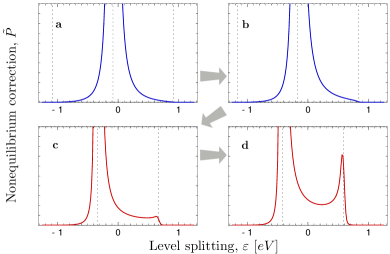
Figure 4: The function $\tilde{P}(\varepsilon)$ that contains the effect of the bias voltage $V$. As explained in the text, $\check{s}_{2}^{\dagger}\check{s}_{1}$ was parameterized as in Eq. (26). A value $\phi=\tfrac{\pi}{9}$ is used througout. The values of $\theta$ in (a), (b), (c) and (d) are respectively $\tfrac{\pi}{6}$, $\tfrac{\pi}{3}$, $\tfrac{2\pi}{3}$ and $\tfrac{5\pi}{6}$. When $\theta<\pi/2$, then $\tilde{P}(\varepsilon)$ has a fairly symmetric peak centered at $-eV\theta/2\pi$. The tails of this peak vanish at $\varepsilon\simeq(-\theta/2\pi\pm 1)eV$. When $\theta>\pi/2$, there are two asymmetric peaks at $-eV\theta/2\pi$ and $(1-\theta/2\pi)eV$. The value of $\tilde{P}(\varepsilon)$ is significantly larger for $\varepsilon\in[-eV\theta/2\pi,(1-\theta/2\pi)eV]$ than outside this interval.

In the main text we confined our attention to the one parameter family of scattering matrices

$$\check{s}_{2}^{\dagger}\check{s}_{1}=\left(\begin{array}[]{cc}\cos\phi&i\sin\phi\\ i\sin\phi&\cos\phi\end{array}\right).$$ (25)

For this choice, $\tilde{P}(\tau)$ is a real function of time. For $\theta<\pi/2$ its fluctuations are associated with energies $\sim\pm eV$ due to the transfer of eigenvalues from $1$ to $\cos\phi$ at a rate of one per $h/eV$. For $\phi>\pi/2$ however, $\cos\phi$ is negative and two eigenvalues have to be transfered before the sign of $\tilde{P}(\tau)$ returns to its initial value. The period of fluctuantions of $\tilde{P}(\tau)$ doubles and becomes associated with energies $\pm eV/2$. Because $\tilde{P}(\tau)$ is real, the fluctuations with positive and negative energies are equal: $\tilde{P}(\varepsilon)=\tilde{P}(-\varepsilon)$. This translates into the following feature of the probability $p_{2}$ to find the qubit in state $\left|2\right>$. For $\phi<\pi/2$, $p_{2}(\varepsilon)$ changes from $1$ to $0$ in an energy interval of length $2eV$. For $\phi>\pi/2$, this interval shrinks to $eV$. The boundry of the interval is defined more sharply the closer $\phi$ is to $0$ or $\pi$. The shrinking from $2eV$ to $eV$ of the interval in which $p_{2}$ varies significantly is explained in terms of charge fractionalization: For $\phi>\pi/2$ the excitations in the QPC transmit half the charge of an electron so that the energy that the qubit can absorb from the QPC changes from $eV$ to $eV/2$.

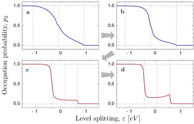
Figure 5: The probability $p_{2}(\varepsilon)$. $\check{s}_{2}^{\dagger}\check{s}_{1}$ is chosen as in Fig. (4): A value $\phi=\tfrac{\pi}{9}$ is used througout. The values of $\theta$ in (a), (b), (c) and (d) are respectively $\tfrac{\pi}{6}$, $\tfrac{\pi}{3}$, $\tfrac{2\pi}{3}$ and $\tfrac{5\pi}{6}$. When $\theta<\pi/2$, the occupation probability $p_{2}$ is significantly different from its asymptotic values $0$ and $1$ in an $\varepsilon$ interval of $2eV$. When $\theta>\pi/2$, this interval shrinks to $eV$. The boundaries of the interval are more sharply defined the closer $\theta$ is to $\pi/2$. The shrinking of the interval corresponds to a cross-over in the QPC from excitations that transmit charge $e$ to excitations that transmit charge $e/2$.

Since the QPC scattering matrices contain parameters that are not under experimental control, it is relevant to ask how the results are altered when a more general choice

$$\check{s}_{2}^{\dagger}\check{s}_{1}=\left(\begin{array}[]{cc}e^{-i\theta}\cos\phi&i\sin\phi\\ i\sin\phi&e^{i\theta}\cos\phi\end{array}\right)$$ (26)

with $\phi\in[-\tfrac{\pi}{2},\frac{\pi}{2}]$ and $\theta\in[0,\pi]$ is made for the scattering matrices. With this choice, eigenvalues travel from $1$ to $e^{i\theta}\cos\phi$ at a rate of one per $2\pi/eV$. This means that the period doubling of $\tilde{P}(\tau)$ no longer takes place. The phase of $\tilde{P}(\tau)$ does not return to its original value after the transfer of two eigenvalues. Rather, one expects fluctuations associated with an energy $(n-\frac{\theta}{2\pi})eV,\ n=0,\pm 1,\pm 2,\ldots$ Because $\tilde{P}(\tau)$ is no longer real, positive and negative frequencies don’t contribute equally. However, while the eigenvalue trajectories lie close to the real line, one can expect results similar to those obtained for real $\tilde{P}(\tau)$. We obtained numerical results for four scattering matrices of the form (26). We chose $\theta=\tfrac{1}{6}\pi,\,\tfrac{1}{3}\pi,\tfrac{2}{3}\pi$ and $\tfrac{5}{6}\pi$. To sharpen abrupt features we chose $\phi=\pi/9$ so that the exponential decay of $\tilde{P}(\tau)$ is associated with a long decoherence time: $\simeq 0.06\hbar/eV$. As depicted in Fig. (4), we found $\tilde{P}(\varepsilon)$ to behave as follows. For $\theta$ close to zero, $\tilde{P}(\varepsilon)$ consists of one peak situated at $\varepsilon=-\frac{\theta}{2\pi}eV$. The tails of this peak vanish at $\varepsilon=\left(\pm 1-\frac{\theta}{2\pi}\right)eV$. The closer to zero that $\theta$ is taken, the more abrupt this behavior of the tails become. As $\theta$ is increased, a second peak starts appearing at $\varepsilon=\left(1-\frac{\theta}{2\pi}\right)eV$. When $\theta=\pi-0^{+}$, the height (and width) of this peak exactly equals that of the peak at $-\frac{\theta}{2\pi}eV$. In the interval $\varepsilon\in\left[-\frac{\theta}{2\pi}eV,\left(1-\frac{\theta}{2\pi}\right)eV\right]$ that is bounded by the peaks, $\tilde{P}(\tau)$ is significantly larger than in the region outside the peaks.

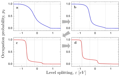
Figure 6: The probability $p_{2}(\varepsilon)$ with spin included. $\check{s}_{2}^{\dagger}\check{s}_{1}$ is chosen as in Fig. (4) and (5): A value $\phi=\tfrac{\pi}{9}$ is used througout. The values of $\theta$ in (a), (b), (c) and (d) are respectively $\tfrac{\pi}{6}$, $\tfrac{\pi}{3}$, $\tfrac{2\pi}{3}$ and $\tfrac{5\pi}{6}$. Fractional charge features are still clearly visible for $\theta>\pi/2$.

This behavior of $\tilde{P}(\varepsilon)$ translates into the occupation probabilities $p_{2}(\varepsilon)$ depicted in Fig. (5). For $\theta<\pi/2$, $p_{2}(\varepsilon)$ still changes from unity to zero in an interval of length $2eV$ manifesting excitations with charge $e$ while for $\theta>\pi/2$ the interval shrinks to $eV$, indication half-integer charge. The closer $\theta$ moves to $0$ or $\pi$, the sharper the interval becomes defined. We therefore conclude that the fractional charge phenomenon in the QPC is not confined to the special choice (25) of scattering matrices.

Appendix C Inclusion of spin

Up to this point we have considered spinless electrons in the QPC. In this Appendix we investigate the effect of including spin. We still take the interaction between the QPC and the qubit to be spin independent. However, the mere existence of a spin degree of freedom for QPC electrons doubles the dimension of channel space. The narrowest QPC now has two channels in stead of one and $\tilde{P}_{s=\tfrac{1}{2}}(\tau)=\tilde{P}_{s=0}(\tau)^{2}$, i.e. the determinant $\tilde{P}_{s=\tfrac{1}{2}}(\tau)$ with spin included is the square of the determinant $\tilde{P}_{s=0}(\tau)$ without spin. For real determinants, squaring kills the phase. This means that the observed period doubling for the parametrization of Eq. (25) disappears and with it the half integer charge features of $p_{2}$. Physically, it could be that two charge $e/2$ excitations are transmitted through the QPC simultaneously. However, fractional charge is saved by the fact that, for $\theta\not=0$, $\tilde{P}_{s=0}(\varepsilon)$ has two peaks with different heights. Suppose the relative peak heights are $A$ and $1-A$, i.e.

$$\tilde{P}_{s=0}(\tau)\sim(1-A)e^{i\tfrac{\theta}{2\pi}eV\tau}+Ae^{-(1-\tfrac{\theta}{2\pi})eV\tau}$$ (27)

where $A$ is a real number between $0$ and $\tfrac{1}{2}$. ($A=0$ corresponds to $\theta=0$ while $A=\tfrac{1}{2}$ corresponds to $\theta=\pi$.) It follows that $P_{s=\tfrac{1}{2}}(\varepsilon)$ has three peaks at

1. $\varepsilon=-2\frac{\theta}{2\pi}eV$ with height $(1-A)^{2}$,

2. $\varepsilon=\left(1-2\frac{\theta}{2\pi}\right)eV$ with height $2A(1-A)$

3. and $\varepsilon=\left(2-2\frac{\theta}{2\pi}\right)eV$ with height $A^{2}$

As long as $A$ is small, i.e. $\theta$ is not too close to $\pi$, the first two peaks will dominate the third, and a signature of fractional charge may still be observable in $p_{2}(\varepsilon)$. Fig. (6), contains $p_{2}$ calculated for the same scattering matrices as in Fig. (5), but with spin included. The cases when $\theta=\tfrac{2}{3}\pi$ and $\theta=\tfrac{5}{6}\pi$ still contain clear half-integer charge features. For $\theta$ very close to $\pi$ (not shown) these features disappear.

References

- (1) B. J. Van Wees et al., Phys. Rev. Lett. 60 848 (1988).
- (2) M. Büttiker, Phys. Rev. B 41 7906 (1990).
- (3) L. S. Levitov, H. Lee and G. H. Lesovik, J. Math. Phys. 37 4845 (1996).
- (4) C. W. J. Beenakker, C. Emary and M. Kindermann, Phys. Rev. Lett. 91, Art. No. 147901 (2003).
- (5) J. M. Elzerman, Phys. Rev. B 67 Art. No. 161308(R) (2003).
- (6) J. R. Petta eta. Phys. Rev. Lett. 93 Art. No. 186802 (2004).
- (7) I. L. Aleiner, I. L., N. S. Wingreen and Y. Meir, Phys. Rev. Lett. 79 3740 (1997).
- (8) Y. Levinson, Europhys. Lett. 39 299 (1997)
- (9) E. Onac, Phys. Rev. Lett. 96 Art. No. 176601 (2006).
- (10) J. Tobiska, J. Danon, I. Snyman and Y. V. Nazarov, Phys. Rev. Lett. 96 Art. No. 096801 (2006).
- (11) R. B. Laughlin, Phys. Rev. Lett. 50 1395 (1983).
- (12) R. Jackiw and C. Rebbi, Phys. Rev. D 13 3398 (1976).
- (13) B. Sutherland and B. S. Shastry, Phys. Rev. Lett. 65, 1833 (1990).
- (14) Y. V. Nazarov and M. Kindermann, Euro. Phys. J. B 35, 413 (2003).
- (15) D. A. Abanin and L. S. Levitov, Phys. Rev. Lett. 93 Art. No. 126802 (2004).
- (16) D. A. Abanin and L. S. Levitov, Phys. Rev. Lett. 94 Art. No. 186803 (2005).
- (17) P. W. Anderson, Phys. Rev. Lett. 24 1049 (1967).
- (18) G. D. Mahan, Phys. Rev. 163 612 (1967).
- (19) P. Nozières and C. T. De Dominicic, Phys. Rev. 178 1097-1107 (1969).
- (20) K. A. Matveev and A. I. Larkin, Phys. Rev. B 46 15337-15347 (1992).
- (21) K. Yamada and K. Yosida, Prog. Th. Phys. 68 1504 (1982).