Excitation spectra and ground state properties of the layered spin-$1/2$ frustrated antiferromagnets Cs₂CuCl₄ and Cs₂CuBr₄

Abstract

We use series expansion methods to study ground- and excited-state properties in the helically ordered phase of spin-$1/2$ frustrated antiferromagnets on an anisotropic triangular lattice. We calculate the ground state energy, ordering wavevector, sublattice magnetization and one-magnon excitation spectrum for parameters relevant to Cs₂CuCl₄ and Cs₂CuBr₄. Both materials are modeled in terms of a Heisenberg model with spatially anisotropic exchange constants; for Cs₂CuCl₄ we also take into account the additional Dzyaloshinskii-Moriya (DM) interaction. We compare our results for Cs₂CuCl₄ with unpolarized neutron scattering experiments and find good agreement. In particular, the large quantum renormalizations of the one-magnon dispersion are well accounted for in our analysis, and inclusion of the DM interaction brings the theoretical predictions for the ordering wavevector and the magnon dispersion closer to the experimental results.

I Introduction

The study of frustrated quantum antiferromagnets is central to modern condensed matter physics. Much of the interest in these many-body systems stems from the possibility, first envisaged by Anderson,andfaz that their quantum fluctuations may be so strong as to lead to exotic “spin-liquid” ground states characterized by the absence of broken symmetries of any kind. Another hallmark signature of spin liquids is the existence of deconfined fractionalized spin-$1/2$ excitations, usually referred to as spinons. Unfortunately it has been very hard to find experimental realizations of such states. Important progress has however been made recently with the identification of some materials which may have, or at least be close to having, a spin-liquid ground state. Two such promising candidates are the organic compound $\kappa$-(BEDT-TTF)₂Cu₂(CN)₃shimizu and the layered $S=1/2$ frustrated antiferromagnet Cs₂CuCl₄.

The magnetic properties of Cs₂CuCl₄ have been extensively studied using neutron scattering.coldea At low temperatures $T<T_{N}=0.62$ K long-range helical magnetic order is observed and the low-energy excitation spectra contain relatively sharp modes characteristic of magnons, the expected Goldstone modes. The magnon dispersion does however show very strong renormalizations compared to linear spin-wave theory. Furthermore, the dominant feature of the spectra is in fact a broad continuum, occurring at medium to high energies, which carries most of the spectral weight and which persists also for temperatures above $T_{N}$. The interpretation of this continuum has recently been the subject of much debate.coldea ; chung1 ; bocquet ; zhouwen ; chung2 ; isakov ; veillette ; dalidovich ; alicea ; yunsor ; sb

The most interesting hypothesis, already suggested in Ref. coldea, , is that the continuum is due to two-spinon scattering resulting from Cs₂CuCl₄ being close to a quantum phase transition to a two-dimensional spin-liquid state. A number of theoretical proposals have been made regarding the nature of the spin liquid that might be involved in such an unconventional scenario.chung1 ; zhouwen ; chung2 ; isakov ; alicea ; yunsor An alternative hypothesis, that the effects of magnon-magnon scattering included within a standard (nonlinear) spin-wave approach might be able to explain the experimental results, was recently explored in Refs. veillette, and dalidovich, . While qualitative features of the calculated spectra were found to be similar to the experimental ones, the quantitative agreement was however not satisfactory. In particular, the obtained quantum renormalization of the magnon dispersion (calculated to lowest order in magnon-magnon interactions) was significantly lower than found experimentally.

The magnetic interactions in Cs₂CuCl₄ are sufficiently weak that the external magnetic field required to fully polarize the spins is experimentally accessible. By measuring the magnon dispersion relation in this fully-polarized state (in which quantum fluctuations are completely suppressed by the applied field), it was foundcoldea-prl-02 that the layers in Cs₂CuCl₄ are nearly decoupled from each other and well described by a spin-$1/2$ triangular-lattice Heisenberg antiferromagnet with exchange constants $J$ and $J^{\prime}$ (defined in Fig. 1) with $J^{\prime}/J\approx 1/3$, weakly perturbed by an additional intra-layer interaction of Dzyaloshinskii-Moriya (DM) type,dm of strength $D/J\approx 0.05$. Although weak, the DM interaction has several important consequences, one being that the ordering plane of the spins coincides with the plane of the triangular lattice because the DM interaction makes the latter an“easy” plane.

Theoretical studies of Cs₂CuCl₄ and models relevant to it have been carried out using many different methods. For the zero-field case, which is our focus here, these methods include spin-wave theory,merino ; veillette ; dalidovich series expansions,zheng99 variational approaches,yunoki ; yunsor and various field-theoretical approaches.chung1 ; bocquet ; zhouwen ; chung2 ; isakov ; alicea ; sb ; ceccatto While most of these studies only considered the Heisenberg part of the Hamiltonian, some of them also investigated the effects of the DM interaction. Refs. veillette, and dalidovich, , using the nonlinear spin-wave approach, found that several quantities, including the ordering wavevector and the quantum renormalization of the magnon dispersion, were quite sensitive to the DM interaction, and that the reduced spin rotation symmetry of the Hamiltonian for $D\neq 0$ also leads to a gap in the magnon dispersion at the ordering wavevector. Ref. dalidovich, also studied the sublattice magnetization as a function of $D$ (for values of $J$, $J^{\prime}$ appropriate for Cs₂CuCl₄) and found that it vanishes when $D/J<0.008$, and hence that the DM interaction is crucial to stabilize the magnetic order in Cs₂CuCl₄. The same qualitative conclusion was reached in Ref. sb, which used a quasi-one-dimensional approach, treating the interchain interactions ($J^{\prime}$ and $D$) using a perturbative renormalization group analysis; these authors found that in the absence of the DM interaction the ground state was dimerized. Finally, the easy-plane nature of the Hamiltonian when $D\neq 0$ plays an essential role in the algebraic vortex-liquid scenario proposed for Cs₂CuCl₄ in Ref. alicea, ; also in this study the magnetic order was found to be driven by the DM interaction.

Another interesting material is Cs₂CuBr₄, which can be described in terms of a spin-$1/2$ triangular-lattice Heisenberg antiferromagnet with $J^{\prime}/J\approx 1/2$.zheng05hight Compared to Cs₂CuCl₄ this material is therefore more frustrated (i.e., closer to the isotropic limit $J=J^{\prime}$) and further away from the one-dimensional limit $J\gg J^{\prime}$. The thermodynamic properties of both materials, particularly the uniform magnetic susceptibility, have been extensively studied. There are also a large number of organic materials from superconducting families that have insulating magnetic phases that can be described by a spatially anisotropic triangular-lattice model.powell Recent high temperature series expansion studies of these systemszheng05hight found that a large class of the organic materials appeared close to the isotropic triangular-lattice limit, while the inorganic materials were closer to the one-dimensional limit.

In this paper we study spin-$1/2$ triangular-lattice antiferromagnets using zero-temperature high-order series expansions. We focus on the case $J>J^{\prime}$ for which, according to our previous series expansion study in Ref. zheng99, , the ground state has noncollinear (helical) long-range magnetic order and the ordering wave vector varies continuously with the model parameters. We calculate the ground state energy, ordering wavevector, sublattice magnetization, and magnon dispersion for values of $J^{\prime}/J$ relevant to Cs₂CuCl₄ and Cs₂CuBr₄. For Cs₂CuCl₄ we also consider the effects of the DM interaction. We compare our results with those of other theoretical approaches and with neutron scattering experiments. A few of the results discussed in this paper have already been briefly presented in Ref. zheng06, .

The outline of the paper is as follows. In Sec. II we describe the model Hamiltonian. In Sec. III we discuss the series expansion method used for studying zero-temperature properties in the helical phase. In Secs. IV and V we discuss our results for ground state properties and the magnon dispersion, respectively. Finally, our conclusions are presented in Sec. VI.

Figure 1: Exchange constants $J$, $J^{\prime}$ and lattice basis vectors $\bm{\delta}_{1}$, $\bm{\delta}_{2}$ on a triangular lattice. The standard notation for axes in Cs₂CuCl₄ is also indicated.

II Model Hamiltonian

The antiferromagnetic spin-$1/2$ Heisenberg model with spatially anisotropic exchange constants on a triangular lattice forms the basis for a theoretical description of the magnetic properties of both Cs₂CuCl₄ and Cs₂CuBr₄. The Heisenberg Hamiltonian reads

$$H_{\text{H}}=\sum_{\bm{R}}[J\;\bm{S}_{\bm{R}}\cdot\bm{S}_{\bm{R}+\bm{\delta}_{1}+\bm{\delta}_{2}}+J^{\prime}\;\bm{S}_{\bm{R}}\cdot(\bm{S}_{\bm{R}+\bm{\delta}_{1}}+\bm{S}_{\bm{R}+\bm{\delta}_{2}})],$$ (1)

where $\bm{S}_{\bm{R}}$ is the spin operator on site $\bm{R}$, $J$ and $J^{\prime}$ are the antiferromagnetic exchange constants, and $\bm{\delta}_{1}$ and $\bm{\delta}_{2}$ are nearest-neighbor lattice vectors, as defined in Fig. 1.

When the ground state of $H_{\text{H}}$ has magnetic long-range order, the spin expectation value can be written

$$\langle\bm{S}_{\bm{R}}\rangle=M[\bm{n}_{1}\cos(\bm{Q}\cdot\bm{R})+\bm{n}_{2}\sin(\bm{Q}\cdot\bm{R})]$$ (2)

where $M$ is the sublattice magnetization, $\bm{n}_{1}$ and $\bm{n}_{2}$ are two arbitrary orthogonal unit vectors, and $\bm{Q}=(0,Q,0)$ is the ordering wavevector with $\cos(Qb/2)=\cos q$, where $q$ ($2q$) is the angle between nearest-neighbor spins coupled by $J^{\prime}$ ($J$) and $b$ is the lattice constant in the $\hat{b}$ direction (see Fig. 1). For classical spins (corresponding to the limit of spin $S\to\infty$), $M=S$ and $q=\arccos(-J^{\prime}/2J)$ (for $J>J^{\prime}/2$). Eq. (2) then implies that the magnetic order is helical, with the ordering plane spanned by the vectors $\bm{n}_{1}$ and $\bm{n}_{2}$. For quantum spins, quantum fluctuations could in principle kill the magnetic order. However, in one of our earlier series expansion studieszheng99 of the model (1) for $S=1/2$, the magnetic order appeared to be robust as long as $J/J^{\prime}$ is not too large. The quantum fluctuations do however renormalize $Q$ (and hence $q$) away from the classical value and reduce the strength of the ordering so that the sublattice magnetization $M<S$.

Cs₂CuBr₄ can be described by the Hamiltonian (1) with $J/J^{\prime}\approx 2$.zheng05hight In contrast, Cs₂CuCl₄ has $J=0.374(5)$ meV and $J^{\prime}=0.128(5)$ meV, giving a more anisotropic ratio $J/J^{\prime}\approx 2.92$.coldea-prl-02 Furthermore, the spin Hamiltonian of Cs₂CuCl₄ also contains a Dzyaloshinskii-Moriya (DM) interactiondm $H_{\text{DM}}$ of the formcoldea-prl-02

$$H_{\text{DM}}=\sum_{\bm{R}}\bm{D}\cdot\bm{S}_{\bm{R}}\times(\bm{S}_{\bm{R}+\bm{\delta}_{1}}+\bm{S}_{\bm{R}+\bm{\delta}_{2}}),$$ (3)

where $\bm{D}$ lies along the $a$-direction, perpendicular to the plane of the triangular lattice, with $D=0.020(2)$ meV, giving $D/J^{\prime}\approx 0.16$. Thus the DM interaction is numerically a relatively small perturbation on the dominant Heisenberg Hamiltonian $H_{H}$. Nevertheless, the DM interaction has several notable consequences. It breaks the full SU(2) spin rotation symmetry of the Heisenberg part down to $U(1)$ by making the plane of the triangular lattice an ”easy plane” which therefore becomes the ordering plane of the spins. Furthermore, as the DM interaction can be seen to give rise to a linear coupling to the unit vector $\bm{n}_{1}\times\bm{n}_{2}$ (which points perpendicular to the ordering plane), it selects a unique direction for this vector, corresponding to a specific chirality or handedness of the spin order. In Cs₂CuCl₄ the direction of $\bm{D}$ in fact alternates from layer to layercoldea-prl-02 and hence the chirality alternates as well.

When discussing Cs₂CuCl₄ in this paper we will consider both the Hamiltonian $H_{\text{H}}+H_{\text{DM}}$ with $D/J^{\prime}=0.16$ as well as the more simplified model defined by neglecting the DM interaction, i.e., $D=0$. In Cs₂CuCl₄ there is also an antiferromagnetic interlayer exchange interaction $J^{\prime\prime}$,coldea-prl-02 but because this is very small ($J^{\prime\prime}=0.017(2)$ meV $\approx J/45$) and because its effectiveness in coupling the layers is further reduced by the alternating chirality, we choose not to include this interlayer interaction in our analysis, thus focussing on a single layer.

III Series expansions in the helically ordered phase

In this section we discuss some aspects of the series expansion analysis of the helically ordered phase.

Following Ref. zheng0608008, , we assume that the spins order in the $xz$ plane (which would be the $bc$ plane in Cs₂CuCl₄), with $\bm{D}$ pointing in the perpendicular direction. We rotate all the spins so as to have a ferromagnetic ground state, with the resulting Hamiltonian $H$:

$$H=H_{1}+JH_{2}+H_{3}$$ (4)

where

$$H_{1}=J\cos{(2q)}\sum_{\langle in\rangle}S^{z}_{i}S^{z}_{n}+[J^{\prime}\cos{(q)}-D\sin(q)]\sum_{\langle ij\rangle}S^{z}_{i}S^{z}_{j},$$ (5)

$$H_{2}=\sum_{\langle in\rangle}S_{i}^{y}S_{n}^{y}+\cos{(2q)}S_{i}^{x}S_{n}^{x}+\sin{(2q)}(S_{i}^{z}S_{n}^{x}-S_{i}^{x}S_{n}^{z}),$$ (6)

$$H_{3} = \sum_{\langle ij\rangle}J^{\prime}S_{i}^{y}S_{j}^{y}+[J^{\prime}\cos{(q)}-D\sin(q)]S_{i}^{x}S_{j}^{x}$$ (7)

$$+[J^{\prime}\sin{(q)}+D\cos(q)](S_{i}^{z}S_{j}^{x}-S_{i}^{x}S_{j}^{z}).$$

where the sum $\langle in\rangle$ is over nearest-neighbor sites connected by “horizontal” bonds in Fig. 1 with exchange interaction $J$, and the sum $\langle ij\rangle$ is over nearest-neighbor sites connected by “diagonal” bonds with exchange interaction $J^{\prime}$.

Next, we introduce the Hamiltonian

$$H(\lambda)\equiv H_{0}+\lambda V$$ (8)

where

$$H_{0}=H_{1}-t\sum_{i}(S_{i}^{z}-1/2),$$ (9)

$$V=JH_{2}+H_{3}+t\sum_{i}(S_{i}^{z}-1/2).$$ (10)

The last term of strength $t$ in both $H_{0}$ and $V$ is a local field term, which can be included to improve convergence. $H(\lambda=0)$ is a ferromagnetic Ising model with two degenerate ground states, while $H(\lambda=1)$ is the model whose properties we are interested in. We use linked-cluster methods to develop series expansion in powers of $\lambda$ for ground state properties and the magnon excitation spectra.

For $J\neq J^{\prime}$, the lattice has $C_{2v}$ symmetry (the symmetry operations are the identity, inversion, and reflections about the $b$ and $c$ axes), and the series for the spin-triplet excitation spectra has the following form:

$$\omega(k_{x},k_{y})/J^{\prime}=\sum_{r=0}^{\infty}\lambda^{r}\sum_{m,n}c_{r,m,n}\cos(\frac{m}{2}k_{x})\cos(\frac{n\sqrt{3}}{2}k_{y})$$ (11)

where $c_{r,m,n}$ are series coefficients, $m$ and $n$ are integers, representing a hopping over distance $(m/2,n\sqrt{3}/2)$, and $m+n$ is a even number. For this case, series for the spin-triplet dispersion has been computed to order $\lambda^{8}$, and the calculations involve a list of 25022 linked-clusters, up to 9 sites. The series coefficients $c_{r,m,n}$ for $J=2.92$, $J^{\prime}=1$, $q=1.64$, $D=0.16$, and $t=4$ are given in Table 2.

For more details we refer to Ref. zheng0608008, where series expansions for the ground state properties and magnon disperion of the spin-$1/2$ Heisenberg model on the anisotropic triangular lattice are discussed at length.oitmaa

Figure 2: The ground state energy per site, as a function of the angle $q$ between nearest-neighbor spins along $J^{\prime}$ bonds, obtained from the series expansion around the Ising limit. (a) $J/J^{\prime}=2$, relevant for Cs₂CuBr₄. Here the left and right vertical dashed lines denote the value of $q$ obtained from dimer expansions [Eq. (16) in Ref. zheng99, ], and the classical ground state, respectively. (b) $J/J^{\prime}=2.92$, the ratio appropriate for Cs₂CuCl₄. The DM interaction ($D=0.16J^{\prime}$) lowers the ground state energy and shifts the ordering angle from $q\approx 1.59$ to $q\approx 1.64$.

IV Ground state properties

IV.1 Ordering wavevector

In Fig. 2 we present results for the ground state energy per site, as a function of the ordering angle $q$, for various model parameters. The actual, realized, value of $q$ is that which minimizes the ground state energy.

Cs₂CuBr₄ [Fig. 2(a)]. The value of $q$ predicted by the Ising expansion is seen to be considerably smaller than the classical value (right dashed line) but is quite close to the value predicted from a dimer expansion (left dashed line; Eq. (16) in Ref. zheng99, ).

Cs₂CuCl₄ [Fig. 2(b)]. The ordering wavevector $Q$ (equivalently, the ordering angle $q$) is conventionally expressed in terms of the incommensuration $\epsilon$, defined as the deviation between $Q$ and the antiferromagnetic (with respect to the $b$ direction) wavevector $\pi/b$, measured in units of $2\pi/b$: $\epsilon\equiv(Q-\pi/b)/(2\pi/b)=q/\pi-1/2$. For $D=0$ the series calculation gives $q\approx 1.59$ which implies $\epsilon\approx 0.006$, while for $D/J^{\prime}=0.16$, $q\approx 1.64$ which gives $\epsilon\approx 0.022$. Thus inclusion of the DM interaction increases the incommensuration and brings it much closer to the experimental value $\epsilon=0.030(2)$.coldea-prl-02

In Table 1 we compare our results for the incommensuration $\epsilon$ for the helically ordered phase in Cs₂CuCl₄ with experiments and with predictions from some other theoretical approaches.

IV.2 Sublattice magnetization

For Cs₂CuCl₄ ($J/J^{\prime}=2.92$ and $D/J^{\prime}=0.16$) we find the sublattice magnetization to be $M=0.213(10)$. In this result the main source of error is the uncertainty in the angle $q$. It is interesting to compare this with predictions from other theoretical approaches (see Table 1). In particular, by using the $1/S$ expansion and taking into account quantum corrections up to and including order $1/S^{2}$ to the classical result, Ref. dalidovich, found the slighly smaller value $M\approx 0.18$ for the same parameters, and also predicted that $M=0$ for $D=0$, i.e. that quantum fluctuations would be strong enough to completely melt the magnetically ordered state in the absence of the DM interaction. In contrast, our analysis indicates a small but nonzero value $M\approx 0.10$ for the magnetization when $D=0$, although it should be noted that the error bars are significant (see Fig. 6 in Ref. zheng99, ). We conclude that in both approaches the DM interaction is found to cause a considerable suppression of quantum fluctuations and strengthen the magnetic ordering tendencies. Including the interlayer coupling $J^{\prime\prime}$ is not expected to change the magnitude of the ordered moment by much, as $J^{\prime\prime}$ is rather small ($J^{\prime\prime}/J\sim 45$) and also because the chirality of the spin ordering is opposite in neighboring layers such that the interlayer coupling energy in fact vanishes at the mean field level.

For Cs₂CuBr₂ ($J/J^{\prime}=2$ and $D=0$) series expansions predict $M\approx 0.17$.zheng99 It would be interesting to make precise neutron scattering measurements of the magnitude of the ordered spin moment in both Cs₂CuCl₄ and Cs₂CuBr₄ to compare directly with the theoretical calculations presented here.

Table 1: Comparison of values for the incommensuration $\epsilon$ and sublattice magnetization $M$ for Cs₂CuCl₄ obtained from experiments and various theoretical approaches. Unless noted otherwise, the values of the exchange interactions $J$ and $J^{\prime}$ used in the theoretical calculations are $J=0.374$ meV and $J^{\prime}=0.128$ meV, corresponding to a ratio $J/J^{\prime}=2.92$. $D$ denotes the strength of the Dzyaloshinskii-Moriya interaction.

	$\epsilon$		$M$
	$D=0.16J^{\prime}$	$D=0$	$D=0.16J^{\prime}$	$D=0$
Experiment	0.030(2)coldea-prl-02	N/A		N/A
Classical	0.0533	0.0547	0.5	0.5
$+1/S$ correction	0.031veillette ; dalidovich	0.022dalidovich	$\approx 0.25$vcc ; dalidovich	$\approx 0.07$merino ; dalidovich
$+1/S^{2}$ correction		0.011dalidovich	$\approx 0.18$dalidovich	0dalidovich
Series	0.022	0.006	0.213	$\approx$ 0.1
Variational RVB		0.018yunoki		0yunsor

V Magnon dispersion

V.1 Cs₂CuCl₄

In this subsection we present series expansion results for the magnon dispersion for parameters relevant to Cs₂CuCl₄, discuss the effects of the DM interaction on this dispersion, and compare it to the dispersion obtained from spin-wave theory with $1/S$ correctionsveillette ; dalidovich and to the experimental dispersion obtained from inelastic neutron scattering with unpolarized neutrons.coldea

V.1.1 Series dispersion

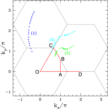
Figure 3: (Color online) Reciprocal space diagram for the triangular lattice. The path ABCOAD ($A=(\pi,0)$, $B=(\pi,\pi/\sqrt{3})$, $C=(2\pi/3,2\pi/\sqrt{3})$, $O=(0,0)$, and $D=(2\pi,0)$) and the three sets of points denoted (1)-(3) are cuts along which magnon dispersions are plotted in subsequent figures in the paper.

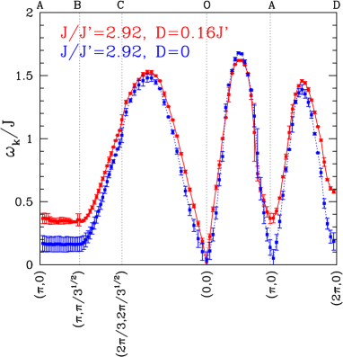
Figure 4: (Color online) Magnon dispersion $\omega_{\bm{k}}$, as calculated from series expansions, for parameters relevant to Cs₂CuCl₄, plotted along the path ABCOAD shown in Fig. 3. When the DM interaction is included the magnon energy is significantly enhanced along AB and near the point D, and a gap opens up at the ordering wavevector $\bm{k}=\bm{Q}$.

In Fig. 4 we show series expansion results for the magnon dispersion along the $\bm{k}$-space path ABCOAD in Fig. 3. The dashed blue curve is for $J/J^{\prime}=2.92$ and $D=0$, while the full red curve includes the effect of a finite $D/J^{\prime}=0.16$. We note the following features:

(i) Along AB, which is perpendicular to the chain direction ($b$ axis), the excitation energy for $D/J^{\prime}=0.16$ is significantly enhanced (by more than a factor of two) over that for $D=0$. The dispersion along AB is very flat in both cases.

(ii) The $D\neq 0$ dispersion has a gap at $\bm{k}=\bm{Q}$ while the $D=0$ dispersion is gapless there. This follows from symmetry arguments. For $D=0$ the model has full SU(2) spin rotation symmetry. The helical order then leads to gapless excitations (Goldstone modes) at $\bm{k}=0$ and at the ordering vector $\bm{k}=\bm{Q}$ . The Goldstone mode at $\bm{k}=\bm{Q}$ is associated with rotations of the ordering plane of the spins, which is arbitrary when $D=0$. The SU(2) symmetry is broken by the the DM interaction which fixes the ordering plane to coincide with the plane of the triangular lattice. Thus rotations of the ordering plane costs a finite energy for $D\neq 0$, which creates a gap in the magnon dispersion at $\bm{k}=\bm{Q}$.nagamiya ; rastelli ; vcc ; veillette (It is important to note, however, that to get gapless excitations at the appropriate $\bm{k}$ vectors in the series calculations we need to bias the analysis as discussed in some detail in Ref. zheng0608008, ; an unbiased analysis always gives a gap.)

(iii) Near the point D the excitation energy for $D/J^{\prime}=0.16$ is significantly enhanced (by approximately a factor of three) over the $D=0$ case.

(iv) Overall, the high-energy parts of the dispersion are quite insensitive to the DM interaction, while the low-energy parts are quite sensitive. A notable exception to the latter is the region around $\bm{k}=0$, since the Goldstone theorem dictates gapless excitations at $\bm{k}=0$ regardless of whether $D$ is zero or not (this is because the $\bm{k}=0$ Goldstone mode is associated with long-wavelength rotations of the spins within their ordering planenagamiya ; rastelli ; veillette ; vcc ).

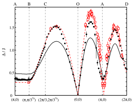
Figure 5: (Color online) Magnon dispersion for $J/J^{\prime}=2.92$ and $D/J^{\prime}=0.16$ (solid points from series, black solid line from spin-wave theory with $1/S$ correction) compared to experimental dispersion in Cs₂CuCl₄ (squares from Ref. coldea, , dashed line is experimental parameterization) along the path ABCOAD in Fig. 3. Compared to the dispersion from spin-wave theory, the series dispersion is enhanced along the $J$ bonds and decreased perpendicular to them. Note that theoretical and experimental dispersions cannot be directly compared near the ordering wavevector $\bm{k}=\bm{Q}$, as the gap in $\omega_{\bm{k}}$ expected at this wavevector cannot be resolved in the unpolarized neutron scattering experiments (see text about how the experimental dispersion is extracted).

V.1.2 Comparison with spin-wave theory

Next we compare our theoretical dispersion for $D/J^{\prime}=0.16$ with that obtained from spin-wave theory with $1/S$ corrections (LSWT + $1/S$ for short).veillette ; dalidovich Both dispersions are plotted in Fig. 5 (black dots and full line, respectively). We see that compared to the spin-wave prediction, the excitation energy is increased in the $b$ direction along which neighboring spins are coupled by the strong $J$ bonds, and decreased in the perpendicular $c$ direction. This corresponds to an upwards renormalization of $J$ and downwards renormalization of $J^{\prime}$ with respect to the spin-wave prediction, which thus effectively makes the system appear more one-dimensional. (The renormalizations of $J$ and $J^{\prime}$ with respect to linear spin-wave theory (LSWT) are even bigger,zheng06 as the LSWT + $1/S$ dispersion itself is in turn characterized by an upwards (downwards) renormalization of $J$ ($J^{\prime}$) compared to LSWT.) The dependence of the magnon energy on the $c$-component of the wavevector is weak, giving the dispersion a pronounced one-dimensional character.

V.1.3 Comparison with experimental dispersion

In Fig. 5 we also show experimental results for the magnon energies obtained from inelastic neutron scattering.coldea The open symbols are data points corresponding to the positions of the strongest peaks in the unpolarized neutron scattering data. The red dashed line is a fit of these points to a dispersion given by

$$\omega_{\bm{k}}=\sqrt{(\tilde{J}_{\bm{k}}-\tilde{J}_{\bm{Q}})\Big{[}(\tilde{J}_{\bm{Q}+\bm{k}}+\tilde{J}_{\bm{Q}-\bm{k}})/2-\tilde{J}_{\bm{Q}}\Big{]}},$$ (12)

where $\tilde{J}_{\bm{k}}=\tilde{J}\cos k_{b}+2\tilde{J^{\prime}}\cos(k_{b}/2)\cos(\sqrt{3}k_{c}/2)$. The functional form of Eq. (12) is identical to the expression from linear spin-wave (LSWT) theory in the absence of the DM interaction, but in Eq. (12) the bare exchange parameters $J$ and $J^{\prime}$ that would be used in LSWT have been replaced by effective, renormalized parameters ($\tilde{J}$ and $\tilde{J}^{\prime}$, respectively) whose values are chosen to give the best fit to the experimental data points. Hence the ratios of these renormalized values to the bare values give a measure of the strength of the quantum fluctuations in the system. In Fig. 5 $\tilde{J}=0.61(1)$ meV and $\tilde{J}^{\prime}=0.107(10)$ meV.coldea

Before comparing the theoretical and experimental curves, however, we first discuss the interpretation of the experimental data in some more detail, i.e. why for a given $\bm{k}$ the location in energy of the strongest peak in the data can in most cases be identified with the magnon energy $\omega_{\bm{k}}$. To this end, we consider the differential cross section for inelastic scattering of unpolarized neutrons, which is proportional tolovesey

$$\sin^{2}\theta_{\bm{k}}\,S^{aa}(\bm{k},\omega)+(1+\cos^{2}\theta_{\bm{k}})\,S^{bb}(\bm{k},\omega)$$ (13)

where $\theta_{\bm{k}}$ is the angle between the scattering wave vector $\bm{k}$ and the axis ($\hat{a}$) perpendicular to the ordering ($bc$) plane of the spins, and $S^{aa}(\bm{k},\omega)$ and $S^{bb}(\bm{k},\omega)$ are diagonal components of the dynamical structure factor defined as ($\mu,\nu=a,b,c$)

$$S^{\mu\nu}(\bm{k},\omega)=\frac{1}{2\pi}\int_{-\infty}^{\infty}dt\;\sum_{\bm{R}}\langle S^{\mu}(0,0)S^{\nu}(\bm{R},t)\rangle e^{-i(\bm{k}\cdot\bm{R}-\omega t)}.$$ (14)

When $\bm{k}$ is in the $bc$ plane (as in our calculations), $\theta_{\bm{k}}=\pi/2$, in which case Eq. (13) reduces to

$$S^{aa}(\bm{k},\omega)+S^{bb}(\bm{k},\omega).$$ (15)

Spin-wave theory predicts sharp one-magnon peaks in the out-of-plane correlations $S^{aa}(\bm{k},\omega)$ at $\omega=\omega_{\bm{k}}$ (referred to as the principal mode) and in the in-plane correlations $S^{bb}(\bm{k},\omega)$ at both $\omega=\omega_{\bm{k}+\bm{Q}}\equiv\omega_{\bm{k}}^{+}$ and $\omega=\omega_{\bm{k}-\bm{Q}}\equiv\omega_{\bm{k}}^{-}$ (referred to as the two secondary modes), where $\omega_{\bm{k}}$ is the magnon dispersion. Hence if the spin-wave prediction for Eq. (15) were plotted as a function of $\omega$ for fixed $\bm{k}$, three peaks would be observed, at $\omega=\omega_{\bm{k}}$ and $\omega_{\bm{k}}^{\pm}$. Although spin-wave theory does not give the correct $\bm{k}$-dependence of the three modes, it is expected that the three-peak structure it predicts (for a system with helical magnetic order) is qualitatively correct. In Fig. 6 we have plotted this structure for $\bm{k}$ varying along the path in Fig. 3 (the energy of the modes was calculated from spin-wave theory with $1/S$ correctionsveillette ). For example, at point B the spin-wave calculation predicts that $\omega_{\bm{k}}$ lies well below the two other modes in energy. This principal mode is also predicted to have the strongest intensity at B. Thus it appears quite safe to assume that the lowest-energy, strongest-intensity peak in the experimental spectrum at that $\bm{k}$-vector should be assigned to $\omega_{\bm{k}}$. At high energies the intensity of the out-of-plane correlations $S^{aa}$ is also predicted to be bigger which justifies an assignment of the location of the strongest peak to $\omega_{\bm{k}}$ at high energies. On the other hand, at low energies close to $\bm{k}=\bm{Q}$, where the primary mode $\omega_{\bm{k}}$ is expected to be gapped and located inside the V-shape of the $\omega_{\bm{k}}^{-}$ mode (see Fig. 6), the $S^{aa}$ part can not be separately resolved. The experimental data indicate that there is no (or very little) overall gap at $k=Q$. This is what one would expect, because for a spiral with finite DM interaction one of the in-plane modes ($\omega_{\bm{k}}^{-}$) would still be gapless.

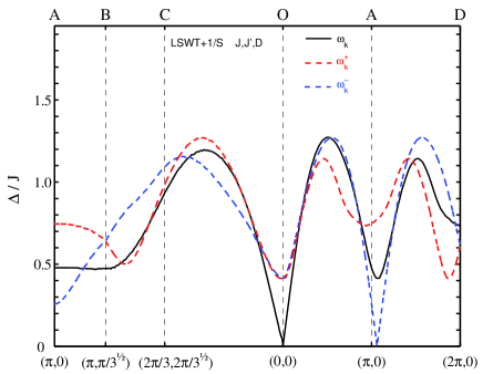
Figure 6: (Color online) The magnon modes $\omega_{\bm{k}}$ (principal mode) and $\omega_{\bm{k}\pm\bm{Q}}\equiv\omega_{\bm{k}}^{\pm}$ (secondary modes), as calculated from spin-wave theory with $1/S$ corrections,veillette for Cs₂CuCl₄ ($J/J^{\prime}=2.92$ and $D/J^{\prime}=0.16$), plotted along the path ABCOAD shown in Fig. 3.

For point B, $\omega_{\bm{k}}$ is quite unambiguously determined, as discussed above, and this point is sensitive to the presence of the DM interaction; the theoretically calculated energy increases with $D$. This makes the interchain dispersion in better agreement with the experimental data when $D$ is included, although there is still a slight overestimate of $\sim 20\%$. Along the AD direction the agreement between experiments and series is essentially perfect, while along the chain direction OA, where the dispersion is maximal, the theory makes a slight underestimate of $\sim 10\%$. The experimental dispersion relation was also measured along off-symmetry directions in the 2D Brillouin zone and Fig. 7 shows that the series results (black circles) compare very well with experimental data (red squares) for those directions too.

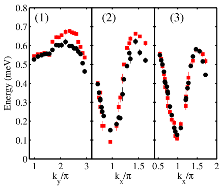
Figure 7: (Color online) Comparison of the experimentally measured dispersion relation in Cs₂CuCl₄ (red squares) and series expansion results for $J=0.385$ meV, $J/J^{\prime}=2.92$ and $D/J^{\prime}=0.16$ (black circles), along paths (1), (2) and (3) in Fig. 3. Calculations were made at the same ($k_{x},k_{y}$) where experimental dispersion points were measured.

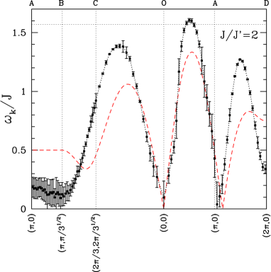
Figure 8: (Color online) Magnon dispersion for Cs₂CuBr₄ ($J=2J^{\prime}$ and $D=0$), calculated from series expansions. Compared to the dispersion from linear spin-wave theory (red dashed line, Eq. (12)) the series dispersion is enhanced along the $J$ bonds and decreased perpendicular to them. The dispersion looks qualitatively rather similar to the case $J/J^{\prime}=2.92$, $D=0$ in Fig. 4 although in that case the energy is practically flat along AB (i.e., perpendicular to the chains) while here the energy varies somewhat along AB, giving a less one-dimensional dispersion, as expected. The horizontal black dashed line is at $\omega/J=\pi/2$ which is the maximum energy in the one-dimensional limit $J/J^{\prime}=\infty$.

V.2 Cs₂CuBr₄

In Fig. 8 we show series expansion results (black symbols) for the magnon dispersion for $J/J^{\prime}=2$, the ratio appropriate for Cs₂CuBr₄, along the $\bm{k}$-space path ABCOAD in Fig. 3. The dispersion obtained from linear spin-wave theory, Eq. (12) is also shown for comparison. We note the following features: (i) With respect to LSWT the series dispersion is renormalized upwards in the direction parallel to the chains (i.e., in the direction along which the exchange constant is strongest) and downwards in the perpendicular direction. A similar kind of upward renormalization occurs both for the square lattice ($J=0$) and decoupled chains ($J^{\prime}=0$). (ii) Along the AB direction perpendicular to the chains, the series dispersion has flattened and the excitation energy has decreased significantly compared to the case $J=J^{\prime}$ case (Fig. 1 in Ref. zheng06, ). Features (i) and (ii) persist as $J/J^{\prime}$ is increased further to 3, as seen in the $D=0$ curve in Fig. 4, which except for the more pronounced flatness along AB looks qualitatively very similar to the $J/J^{\prime}=2$ dispersion in Fig. 8.

VI Conclusions

In this paper we have presented series expansion calculations for various ground state properties (ground state energy, ordering wavevector, and sublattice magnetization), and for the magnon dispersion, in the helically ordered state of spin-$1/2$ frustrated antiferromagnets on an anisotropic triangular lattice. For the parameter values considered here the model Hamiltonians we have studied are expected to give a good description of the magnetic properties of Cs₂CuBr₄ and Cs₂CuCl₄.

For parameters appropriate for Cs₂CuBr₄ ($J/J^{\prime}=2$) we have made specific predictions for large and non-uniform renormalizations of the dispersion relation compared to the classical (linear spin-wave theory) result (see Fig. 8). There is an upward renormalization along the chains and a downward renormalization along the interchain direction. These predictions for Cs₂CuBr₄ should be testable by future neutron scattering experiments.

For Cs₂CuCl₄ we have compared our theoretical predictions for the dispersion with experimental results from neutron scattering experiments and with spin-wave theory that includes $1/S$ corrections. The calculated magnon dispersion shows large quantum renormalizations compared to the classical result; as for Cs₂CuBr₄ the renormalization is upward along the chain direction and downward along the interchain direction. Thus quantum fluctuations make the dispersion look more one-dimensional. These predictions from series are in good quantitative agreement with the experimental observations. In contrast, spin-wave theory with $1/S$ corrections predicts considerably smaller renormalizations and thus underestimates the effects of quantum fluctuations on the dispersion.

The agreement between theory and experiment improves further when the Dzyaloshinskii-Moriya (DM) interaction is taken into account. The DM interaction is found to significantly increase the incommensuration of the ordering wavevector with respect to the antiferromagnetic wavevector in the chain ($\hat{b}$) direction. Another important consequence of the DM interaction is that it opens up a gap in the magnon dispersion at the ordering wavevector. We have made specific predictions for the size of this energy gap at the ordering wavevector to longitudinally-polarized excitations (along the direction normal to the spiral plane) which could be tested by future high-resolution polarized neutron scattering experiments.

Another very interesting issue, at least from a theoretical point of view, is the role of the DM interaction in Cs₂CuCl₄ in stabilizing a magnetically ordered ground state. We find here that inclusion of the DM interaction strengthens the magnetic ordering. In fact, several recent papersdalidovich ; yunsor ; alicea ; sb have predicted that in the absence of the DM interaction the ground state is not magnetically ordered. The proposed alternatives to a magnetically ordered phase for $D=0$ include a spin liquid (“algebraic vortex liquid”)alicea and a state with “staggered” dimerization.sb The latter state could be studied using series expansions; it would be interesting to compare its energy with the helically ordered phase. The fact that a different dimerized state (with “diagonal” dimerization; see Fig. 4a in Ref. zheng99, ) that we have studied with series expansions is extremely close in energy to the helically ordered state (for a large regime of $J/J^{\prime}$ including $J/J^{\prime}\approx 3$ we find that the energies of the two phases lie virtually on top of each other) is strongly suggestive that the state with staggered dimerization proposed in Ref. sb, may be highly competitive as well.

Table 2: Series coefficients for the magnon dispersion for the isotropic triangular-lattice model, calculated for $J=2.92$, $J^{\prime}=1$, $q=1.64$, $D=0.16$, and $t=4$ in Eqs. (9) and (10). Nonzero coefficients $c_{r,m,n}$ in Eq. (11) up to order $r=8$ are listed.

($r,m,n$)	$c_{r,m,n}$	($r,m,n$)	$c_{r,m,n}$	($r,m,n$)	$c_{r,m,n}$	($r,m,n$)	$c_{r,m,n}$
( 0, 0, 0)	7.349606933	( 4, 1, 3)	7.578150248$\times 10^{-4}$	( 4, 7, 1)	-9.342152056$\times 10^{-3}$	( 6, 7, 5)	-1.670797799$\times 10^{-6}$
( 1, 0, 0)	-4.000000000	( 5, 1, 3)	-9.976179492$\times 10^{-4}$	( 5, 7, 1)	-1.835064338$\times 10^{-2}$	( 7, 7, 5)	1.015387605$\times 10^{-6}$
( 2, 0, 0)	6.038563795$\times 10^{-2}$	( 6, 1, 3)	-2.926714357$\times 10^{-3}$	( 6, 7, 1)	-2.367732439$\times 10^{-2}$	( 8, 7, 5)	5.830972082$\times 10^{-6}$
( 3, 0, 0)	-6.217604565$\times 10^{-2}$	( 7, 1, 3)	-4.924224688$\times 10^{-3}$	( 7, 7, 1)	-2.521951807$\times 10^{-2}$	( 6, 8, 4)	-1.600507150$\times 10^{-5}$
( 4, 0, 0)	-1.125358729$\times 10^{-1}$	( 8, 1, 3)	-6.508161119$\times 10^{-3}$	( 8, 7, 1)	-2.415728150$\times 10^{-2}$	( 7, 8, 4)	-2.409589103$\times 10^{-5}$
( 5, 0, 0)	-1.162865812$\times 10^{-1}$	( 3, 3, 3)	6.950474681$\times 10^{-4}$	( 4, 8, 0)	-6.795995712$\times 10^{-3}$	( 8, 8, 4)	-2.189863027$\times 10^{-5}$
( 6, 0, 0)	-9.649286838$\times 10^{-2}$	( 4, 3, 3)	-9.066263964$\times 10^{-4}$	( 5, 8, 0)	-1.353032723$\times 10^{-2}$	( 6, 9, 3)	-8.269690490$\times 10^{-5}$
( 7, 0, 0)	-6.982209428$\times 10^{-2}$	( 5, 3, 3)	-1.496710785$\times 10^{-3}$	( 6, 8, 0)	-1.705500588$\times 10^{-2}$	( 7, 9, 3)	-1.831650139$\times 10^{-4}$
( 8, 0, 0)	-4.568446552$\times 10^{-2}$	( 6, 3, 3)	-5.060095359$\times 10^{-4}$	( 7, 8, 0)	-1.715246720$\times 10^{-2}$	( 8, 9, 3)	-2.277789431$\times 10^{-4}$
( 1, 1, 1)	7.712345303$\times 10^{-1}$	( 7, 3, 3)	1.528045822$\times 10^{-3}$	( 8, 8, 0)	-1.507009210$\times 10^{-2}$	( 6,10, 2)	-2.517791809$\times 10^{-4}$
( 2, 1, 1)	-1.685921734$\times 10^{-1}$	( 8, 3, 3)	3.781329536$\times 10^{-3}$	( 5, 1, 5)	1.418417481$\times 10^{-5}$	( 7,10, 2)	-6.579095073$\times 10^{-4}$
( 3, 1, 1)	-2.106120525$\times 10^{-1}$	( 3, 4, 2)	8.064630409$\times 10^{-3}$	( 6, 1, 5)	7.457692880$\times 10^{-6}$	( 8,10, 2)	-9.157527309$\times 10^{-4}$
( 4, 1, 1)	-1.865808906$\times 10^{-1}$	( 4, 4, 2)	8.310784630$\times 10^{-3}$	( 7, 1, 5)	-6.287690575$\times 10^{-6}$	( 6,11, 1)	-4.658726892$\times 10^{-4}$
( 5, 1, 1)	-1.379395553$\times 10^{-1}$	( 5, 4, 2)	9.603610069$\times 10^{-3}$	( 8, 1, 5)	-1.316193701$\times 10^{-5}$	( 7,11, 1)	-1.474734326$\times 10^{-3}$
( 6, 1, 1)	-9.056954635$\times 10^{-2}$	( 6, 4, 2)	1.286421148$\times 10^{-2}$	( 5, 3, 5)	7.092087407$\times 10^{-6}$	( 8,11, 1)	-2.737063946$\times 10^{-3}$
( 7, 1, 1)	-5.546855043$\times 10^{-2}$	( 7, 4, 2)	1.664667471$\times 10^{-2}$	( 6, 3, 5)	-2.077134408$\times 10^{-6}$	( 6,12, 0)	-2.330119692$\times 10^{-4}$
( 8, 1, 1)	-3.373111871$\times 10^{-2}$	( 8, 4, 2)	1.954078358$\times 10^{-2}$	( 7, 3, 5)	-1.309394434$\times 10^{-5}$	( 7,12, 0)	-8.136447772$\times 10^{-4}$
( 1, 2, 0)	1.396200322$\times 10^{-2}$	( 3, 5, 1)	2.242175366$\times 10^{-2}$	( 8, 3, 5)	-1.292053918$\times 10^{-5}$	( 8,12, 0)	-1.712422519$\times 10^{-3}$
( 2, 2, 0)	-1.505333368$\times 10^{-2}$	( 4, 5, 1)	1.427117691$\times 10^{-2}$	( 5, 5, 5)	1.418417481$\times 10^{-6}$	( 7, 1, 7)	1.364242160$\times 10^{-7}$
( 3, 2, 0)	-2.815674423$\times 10^{-4}$	( 5, 5, 1)	-2.602862242$\times 10^{-3}$	( 6, 5, 5)	-5.076936139$\times 10^{-6}$	( 8, 1, 7)	1.106865429$\times 10^{-7}$
( 4, 2, 0)	1.594690655$\times 10^{-2}$	( 6, 5, 1)	-1.521289949$\times 10^{-2}$	( 7, 5, 5)	-7.060086129$\times 10^{-6}$	( 7, 3, 7)	8.185452960$\times 10^{-8}$
( 5, 2, 0)	2.998362910$\times 10^{-2}$	( 7, 5, 1)	-1.993026012$\times 10^{-2}$	( 8, 5, 5)	1.083485410$\times 10^{-6}$	( 8, 3, 7)	1.069367604$\times 10^{-8}$
( 6, 2, 0)	3.941680852$\times 10^{-2}$	( 8, 5, 1)	-1.888733912$\times 10^{-2}$	( 5, 6, 4)	2.746050501$\times 10^{-5}$	( 7, 5, 7)	2.728484320$\times 10^{-8}$
( 7, 2, 0)	4.308338742$\times 10^{-2}$	( 3, 6, 0)	4.006413979$\times 10^{-4}$	( 6, 6, 4)	1.039487431$\times 10^{-5}$	( 8, 5, 7)	-4.924369043$\times 10^{-8}$
( 8, 2, 0)	4.120905564$\times 10^{-2}$	( 4, 6, 0)	-3.331359320$\times 10^{-3}$	( 7, 6, 4)	-1.115844752$\times 10^{-5}$	( 7, 7, 7)	3.897834743$\times 10^{-9}$
( 2, 0, 2)	-2.650432163$\times 10^{-2}$	( 5, 6, 0)	-6.163747248$\times 10^{-3}$	( 8, 6, 4)	6.482844962$\times 10^{-6}$	( 8, 7, 7)	-3.233550435$\times 10^{-8}$
( 3, 0, 2)	3.538137283$\times 10^{-3}$	( 6, 6, 0)	-7.199966978$\times 10^{-3}$	( 5, 7, 3)	2.089666851$\times 10^{-4}$	( 7, 8, 6)	1.034023057$\times 10^{-7}$
( 4, 0, 2)	2.465629073$\times 10^{-3}$	( 7, 6, 0)	-7.409354256$\times 10^{-3}$	( 6, 7, 3)	2.467736333$\times 10^{-4}$	( 8, 8, 6)	-1.557033299$\times 10^{-7}$
( 5, 0, 2)	-1.050320907$\times 10^{-2}$	( 8, 6, 0)	-8.061924799$\times 10^{-3}$	( 7, 7, 3)	-3.668402903$\times 10^{-5}$	( 7, 9, 5)	1.173239911$\times 10^{-6}$
( 6, 0, 2)	-2.242983874$\times 10^{-2}$	( 4, 0, 4)	-9.054115944$\times 10^{-5}$	( 8, 7, 3)	-5.809689111$\times 10^{-4}$	( 8, 9, 5)	7.836228877$\times 10^{-7}$
( 7, 0, 2)	-2.768399107$\times 10^{-2}$	( 5, 0, 4)	-5.479146209$\times 10^{-5}$	( 5, 8, 2)	7.675228288$\times 10^{-4}$	( 7,10, 4)	7.377737697$\times 10^{-6}$
( 8, 0, 2)	-2.619803879$\times 10^{-2}$	( 6, 0, 4)	3.687786670$\times 10^{-6}$	( 6, 8, 2)	1.512127062$\times 10^{-3}$	( 8,10, 4)	1.539074513$\times 10^{-5}$
( 2, 2, 2)	-2.650432163$\times 10^{-2}$	( 7, 0, 4)	-1.852548500$\times 10^{-5}$	( 7, 8, 2)	1.521619340$\times 10^{-3}$	( 7,11, 3)	2.754833548$\times 10^{-5}$
( 3, 2, 2)	-9.979720263$\times 10^{-4}$	( 8, 0, 4)	-1.568789895$\times 10^{-4}$	( 8, 8, 2)	6.001765269$\times 10^{-4}$	( 8,11, 3)	8.079901649$\times 10^{-5}$
( 4, 2, 2)	6.636359222$\times 10^{-3}$	( 4, 2, 4)	-1.207215459$\times 10^{-4}$	( 5, 9, 1)	1.165606703$\times 10^{-3}$	( 7,12, 2)	5.930561117$\times 10^{-5}$
( 5, 2, 2)	5.391428994$\times 10^{-3}$	( 5, 2, 4)	-2.149262987$\times 10^{-5}$	( 6, 9, 1)	2.854089455$\times 10^{-3}$	( 8,12, 2)	1.954393847$\times 10^{-4}$
( 6, 2, 2)	2.036622085$\times 10^{-3}$	( 6, 2, 4)	7.358270843$\times 10^{-5}$	( 7, 9, 1)	4.479815788$\times 10^{-3}$	( 7,13, 1)	5.956579054$\times 10^{-5}$
( 7, 2, 2)	1.434767818$\times 10^{-4}$	( 7, 2, 4)	5.557974820$\times 10^{-5}$	( 8, 9, 1)	5.794251007$\times 10^{-3}$	( 8,13, 1)	1.916748738$\times 10^{-4}$
( 8, 2, 2)	6.693067703$\times 10^{-4}$	( 8, 2, 4)	-3.425847619$\times 10^{-5}$	( 5,10, 0)	2.060334673$\times 10^{-5}$	( 7,14, 0)	1.040120579$\times 10^{-6}$
( 2, 3, 1)	-3.084059676$\times 10^{-1}$	( 4, 4, 4)	-3.018038648$\times 10^{-5}$	( 6,10, 0)	-1.952180586$\times 10^{-4}$	( 8,14, 0)	-1.495168851$\times 10^{-5}$
( 3, 3, 1)	-1.588761190$\times 10^{-1}$	( 5, 4, 4)	6.075933723$\times 10^{-5}$	( 7,10, 0)	-6.035252148$\times 10^{-4}$	( 8, 0, 8)	-7.586845473$\times 10^{-9}$
( 4, 3, 1)	-4.101867358$\times 10^{-2}$	( 6, 4, 4)	1.000503366$\times 10^{-4}$	( 8,10, 0)	-9.362009169$\times 10^{-4}$	( 8, 2, 8)	-1.213894466$\times 10^{-8}$
( 5, 3, 1)	3.354266372$\times 10^{-2}$	( 7, 4, 4)	9.862298579$\times 10^{-5}$	( 6, 0, 6)	-7.263598281$\times 10^{-7}$	( 8, 4, 8)	-6.069460194$\times 10^{-9}$
( 6, 3, 1)	7.243569855$\times 10^{-2}$	( 8, 4, 4)	1.673415457$\times 10^{-4}$	( 7, 0, 6)	-5.650646253$\times 10^{-7}$	( 8, 6, 8)	-1.734128016$\times 10^{-9}$
( 7, 3, 1)	8.854496129$\times 10^{-2}$	( 4, 5, 3)	-4.901068912$\times 10^{-4}$	( 8, 0, 6)	2.353281314$\times 10^{-7}$	( 8, 8, 8)	-2.167670129$\times 10^{-10}$
( 8, 3, 1)	9.234591989$\times 10^{-2}$	( 5, 5, 3)	9.426485008$\times 10^{-5}$	( 6, 2, 6)	-1.089539742$\times 10^{-6}$	( 8, 9, 7)	-6.526162920$\times 10^{-9}$
( 2, 4, 0)	-4.736398330$\times 10^{-1}$	( 6, 5, 3)	1.397521826$\times 10^{-3}$	( 7, 2, 6)	-4.743845804$\times 10^{-7}$	( 8,10, 6)	-8.596029431$\times 10^{-8}$
( 3, 4, 0)	-4.199253740$\times 10^{-1}$	( 7, 5, 3)	2.688369202$\times 10^{-3}$	( 8, 2, 6)	1.060978601$\times 10^{-6}$	( 8,11, 5)	-6.482179010$\times 10^{-7}$
( 4, 4, 0)	-3.246293814$\times 10^{-1}$	( 8, 5, 3)	3.441529158$\times 10^{-3}$	( 6, 4, 6)	-4.358158969$\times 10^{-7}$	( 8,12, 4)	-3.069805782$\times 10^{-6}$
( 5, 4, 0)	-2.188669309$\times 10^{-1}$	( 4, 6, 2)	-3.058604819$\times 10^{-3}$	( 7, 4, 6)	4.028642250$\times 10^{-7}$	( 8,13, 3)	-9.416441458$\times 10^{-6}$
( 6, 4, 0)	-1.251987959$\times 10^{-1}$	( 5, 6, 2)	-4.021118013$\times 10^{-3}$	( 8, 4, 6)	1.336492139$\times 10^{-6}$	( 8,14, 2)	-1.872276535$\times 10^{-5}$
( 7, 4, 0)	-5.434016523$\times 10^{-2}$	( 6, 6, 2)	-2.960843639$\times 10^{-3}$	( 6, 6, 6)	-7.263598281$\times 10^{-8}$	( 8,15, 1)	-2.388666059$\times 10^{-5}$
( 8, 4, 0)	-7.501154228$\times 10^{-3}$	( 7, 6, 2)	-1.581263941$\times 10^{-3}$	( 7, 6, 6)	4.155864858$\times 10^{-7}$	( 8,16, 0)	-8.823605179$\times 10^{-6}$
( 3, 1, 3)	2.085142404$\times 10^{-3}$	( 8, 6, 2)	-1.344189910$\times 10^{-3}$	( 8, 6, 6)	4.410976005$\times 10^{-7}$