Thermal rectifying effect in two dimensional anharmonic lattices

Abstract

We study thermal rectifying effect in two dimensional (2D) systems consisting of the Frenkel Kontorva (FK) lattice and the Fermi-Pasta-Ulam (FPU) lattice. It is found that the rectifying effect is related to the asymmetrical interface thermal resistance. The rectifying efficiency is typically about two orders of magnitude which is large enough to be observed in experiment. The dependence of rectifying efficiency on the temperature and temperature gradient is studied. The underlying mechanism is found to be the match and mismatch of the spectra of lattice vibration in two parts.

I Introduction

Heat conduction in low dimensional systems has attracted increasing attention Peierls55 ; Casati84 ; Prosen92 ; Kaburaki93 ; Lepri97 ; Lepri98 ; SLepri98 ; Lepri03 ; Hu98 ; Fillipov ; Hu00 ; Bonetto00 ; Giardin00 ; Gendelman00 ; Prosen00 ; Aoki ; Li02 ; Alonso02 ; Li03 ; Pereverzev03 ; BLi03 ; Li04 ; Li06 in recent years. After two decades analytic and numerical studies in 1D model, much progress has been achieved. On the one hand, the study has enriched our understanding about the underlying physical mechanism. On the other hand, the study has made it possible to seek the practical application of heat control and management. Indeed, in 2002, Terraneo et al Terraneo02 proposed a thermal device which can rectify the heat current through it when reversing the temperature gradient. The model proposed by Terraneo et al is a 1D anharmonic lattice consisting of three segments with the Morse on-site potential of different parameters. As the first attempt of controlling heat current, the ratio of the thermal current changes is less than two. More recently, Li et al. BLi04 construct a thermal diode model in which two Frenkel-Kontoroval (FK) chains with different nonlinear strengths are connected by a harmonic spring. The most successful improvement of the model by Li et al BLi04 lies in three facts: First, the configuration is more simple, it consists of only two different segments; Second, the ratio of heat current from two different directions is increased drastically about 100 times; Third, the underlying mechanism of thermal rectifying effect is explained by illustrating the phonon bands of the particles in different segments. Following Li et al’s work, we further improve the rectifying efficiency from 100 to 2000 by substituting the weak FK chain with a Fermi-Pasta-Ulam (FPU) chain Li05 . In addition, we find that the rectifying effect (asymmetric heat flow) is closely related to asymmetric interface thermal resistance (also called Kapitza resistance). Moreover, a specific relationship between the ratio of heat current and the overlap of the phonon spectra is demonstrated numerically. The rectifying effect can also be achieved by modulating the periodicity of the on-site potential of the FK lattice Hu05 .

The above works demonstrate the possibility of controlling heat current by changing structures/parameters of anharmonic lattices. These might find potential application in energy saving material. However, almost all works so far are focused on 1D system of finite size. Obviously, much progress has been achieved, but the final purpose is to put these ideas to application. It is thus a nature step forward to seek effective thermal devices to control heat current in higher dimension. The open questions are: whether the heat control mechanism in 1D is still valid for the high dimension(s) and whether the extra dimension(s) reduces the rectifying efficiency? The answer might not be trivial, as in higher dimension the lattice vibration includes not only the longitudinal one but also the transverse ones. The longitudinal modes will couple to the transverse modes Wang04 , which might affect the rectifying efficiency.

In this paper, we concentrate our study on a 2D rectifier model. We will demonstrate with numerical evidence that a 2D rectifier can be built up and it works in a very wide temperature range. The 2D thermal rectifier shows similar behaviors with 1D thermal rectifier under similar parameters regimes.

The paper is organized as the follows. In Section II, we describe our model and numerical method used for the computer simulation. In Section III, we demonstrate and discuss the dependence of the thermal rectifying efficiency on the temperature and the temperature gradient. Section IV is devoted to the interface thermal resistance which is the key point to understand the thermal rectifying effect. In Section V, we give physical understanding of the rectifying effect in terms of the lattice vibration spectra (also called phonon band.) We conclude the paper by conclusions and discussions in Sec. VI.

II Model and methodology

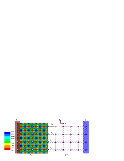
Figure 1: (Color Online) Configuration of a two dimensional (2D) thermal rectifier from the Frenkel Kotoroval and the Fermi-Pasta-Ulam lattices. The left part is a 2D FK lattice and the right one is a 2D Fermi-Pasta-Ulam lattice. The two parts are connected by harmonic springs with constant $k_{int}$. The left and the right ends are put into contact with heat baths of temperature $T_{L}$ and $T_{R}$, respectively.

In our previous workLi05 , we construct a 1D thermal diode model by connecting a FK lattice to a FPU lattice with a weak harmonic spring. We denote it as 1D-FK-FPU model. This model displays a very good rectifying effect. In this paper, we extend the 1D- FK-FPU thermal rectifier model to two dimensional one. We denote it as a 2D-FK-FPU model. The configuration of the 2D-FK-FPU model is illustrated in Fig1. The left part is a plane of harmonic oscillators on a substrate whose interaction is represented by a sinusoidal on-site potential. Here we plot the contour line of the 2D sinusoidal potential. For simplicity, we put one particle in each valley. The right part is an array of an-harmonic oscillators represented by the FPU model. The two parts are connected by weak harmonic springs. The Hamiltonian of the system can be written as:

$$H=H_{FK}+H_{FPU}+H_{int},$$ (1)

where $H_{FK}$, $H_{FPU}$, $H_{int}$ is the Hamiltonian of the left part, the right part and the interface section, respectively. They are represented in (2), (3), (4), respectively.

$$\begin{split}H_{FK}&=\sum_{i=1}^{N_{FK}}\sum_{j=1}^{N_{Y}}(\frac{\vec{p}^{2}_{i,j}}{2}+k_{FK}V_{H}(|\vec{r}_{i,j;i-1,j}|-l_{0})\\ &+k_{FK}V_{H}((|\vec{r}_{i,j;i,j-1}|-l_{0}))+U_{FK}(x_{i,j},y_{i,j}))\end{split}$$ (2)

$$\begin{split}H_{FPU}&=\sum_{i=N_{FK}+1}^{N_{X}}\sum_{j=1}^{N_{Y}}(\frac{\vec{p}^{2}_{i,j}}{2}\\ &+k_{FPU}V_{FPU}(|\vec{r}_{i,j;i-1,j}|-l_{0})\\ &+k_{FPU}V_{FPU}(|\vec{r}_{i,j;i,j-1}|-l_{0}))\end{split}$$ (3)

$$H_{int}=\sum_{j=1}^{N_{Y}}k_{int}V_{H}(|\vec{r}_{N_{FK},j;N_{FK}+1,j}|-l_{0})$$ (4)

where $\vec{r}_{i,j;k,l}=\vec{q}_{i,j}-\vec{q}_{k,l}$ is the relative displacement between particles, labelled as $(i,j)$ and $(k,l)$. $V_{H}(x)=\frac{1}{2}x^{2}$, $V_{FPU}(x)=\frac{1}{2}x^{2}+\frac{1}{4}x^{4}$, $U_{FK}(x,y)=-\frac{A}{(2\pi)^{2}}\cos(\frac{2\pi}{l_{0}}x)\cos(\frac{2\pi}{l_{0}}y)$.

The mass of the particles is uniformly 1. $l_{0}$ is distance between nearest neighbors in equilibrium. The particle at the $i$th column and the $j$th row is labelled as $(i,j)$. The coordinate and momentum of this particle is $\vec{q}_{i,j}=(x_{i,j},y_{i,j})$ and $\vec{p}_{i,j}=(p_{x_{i,j}},p_{y_{i,j}})$. In order to establish a temperature gradient, the two ends of the planes are put into contact with two Nosé-Hoover heat bathesNose with temperature $T_{L}$ and $T_{R}$ for the left end and the right end, respectively. Particles for $i=1,j=1,2,3...N_{Y}$ are coupled with heat bath of temperature $T_{L}$ and particles for $i=N_{X},j=1,2,3...N_{Y}$ are coupled with heat bath of temperature $T_{R}$. We checked in 1D case that the result does not depend on the particular heat bath realization. Fixed boundary condition is used along temperature gradient direction, denoted as $X$ direction in this paper, namely, $\vec{q}_{0,j}=(0,j)$, $\vec{q}_{N_{X}+1,j}=(N_{X}+1,j)$. Periodic boundary condition is applied in the $Y$ direction, namely, $\vec{q}_{i,1}=\vec{q}_{i,N_{Y}+1}$ (see Fig. 1). Under these boundary conditions, the system can be considered as a tube. The total number of particles is $N_{X}\times N_{Y}$. All results given in this paper are obtained by averaging over $N\times 10^{8}$($N>2$)steps after a sufficient long transient time when a non-equilibrium stationary state is set up. The equations of motion of the particles are:

$$\begin{array}[]{c}\dot{\vec{q}}_{i,j}=\vec{p}_{i,j},\\ \\ \dot{\vec{p}}_{i,j}=\left\{\begin{array}[]{ll}-\frac{\partial H}{\partial\vec{q}_{i,j}}(i=2,N_{X}-1),\\ \\ -\frac{\partial H}{\partial\vec{q}_{i,j}}-\xi_{i,j}\vec{p}_{i,j}(i=1,N_{X}).\\ \end{array}\right.\\ \end{array}$$ (5)

and the auxiliary variables $\xi_{i,j}$ are described by the equations:

$$\dot{\xi}_{i,j}=\frac{1}{\mathcal{Q}}(\frac{\vec{p}_{i,j}^{2}}{2k_{B}T}-1),$$ (6)

here, $T$ is the temperature of the heat bath ($T_{L}$ or $T_{R}$), and $\mathcal{Q}$ is the parameter of coupling between the thermal bath and the system. In this study, we set $\mathcal{Q}=1$ so that the response time of the thermostats, $\frac{1}{\sqrt{\mathcal{Q}}}$, is of the same order of the original time scale of the lattice. Our purpose is to study rectifying effect in two dimension and the dependence of the rectifying efficiency on the system temperature and the temperature gradient, so we don’t attempt to search the optimum setting of parameters. We choose the system parameters same as in 1D FK-FPU model which has been tested as good one in 1D case, that is $k_{FK}=1$, $A=5$ , $l_{0}=1$, $k_{FPU}=0.2$ and $k_{int}=0.05$. We set

$$\begin{array}[]{c}T_{L}=T_{0}(1+\Delta),\\ \\ T_{R}=T_{0}(1-\Delta),\end{array}$$ (7)

where $-0.8\leq\Delta\leq 0.8$ in our simulations. So we can simply denote $T_{0}$ as the temperature added on the system and $2\Delta=(T_{R}-T_{L})/T_{0}$ as the normalized temperature difference of the system.

The temperature used in our numerical simulation is dimensionless. It is connected with the true temperature $T_{r}$ through the following relationHu98 , $T_{r}=\frac{m\omega_{0}^{2}b^{2}}{k_{B}}T,$ where $m$ is the mass of the particle and $b$ is the period of external potential. $\omega_{0}$ is the vibration frequency. $k_{B}$ is the Boltzman constant. For the typical values of atoms, we have $T_{r}\sim(10^{2}-10^{3})$Hu98 , which means that the room temperature corresponds to the dimensionless temperature $T\sim(0.1-1)$.

The local temperature is defined as

$$T_{i,j}=\frac{1}{2}m\langle\vec{v}_{i,j}^{2}\rangle,$$ (8)

where $\langle\dots\rangle$ stands for a temporal average. The local heat current $J_{i,j}$ is defined as the energy transfer per unit time from the particle labelled as $(i,j)$ to the nearest particles along $X$ direction.

$$\begin{split}J_{i,j}&=-\vec{v}_{i,j}\cdot\vec{F}_{i,j}\\ &=-k\vec{v}_{i,j}\cdot\frac{\partial\left(V(|\vec{r}_{i+1,j;i,j}|-l_{0})+V(|\vec{r}_{i,j;i-1,j}|-l_{0})\right)}{\partial\vec{q}_{i,j}},\end{split}$$ (9)

where $k=k_{FK},k_{FPU}$ or $k_{int}$, depending on the site along $X$ direction. For a 2D-lattice, we treat only heat current flowing along the $X$-direction. We denote the current from the particles in $i$th section to the next section in the $X$-direction simply as $J_{i}$($J_{i}=\sum_{j=1}^{N_{Y}}J_{i,j}$). The total current of the system is averaged over all sections,

$$J=\frac{1}{N_{X}}\langle\sum_{i=1}^{N_{X}}J_{i}\rangle.$$ (10)

In our simulations, the fluctuations of temporal heat current through each section are all less than five percents. We use $|J_{+}/J_{-}|$ as a rectifying efficiency, to describe quantitatively the rectifying performance of the system. $J_{+}$ is the current when $\Delta$ is positive (heat flows from the FK part to the FPU part) and $J_{-}$ is the current when $\Delta$ is negative (heat flows from the FPU part to the FK part).

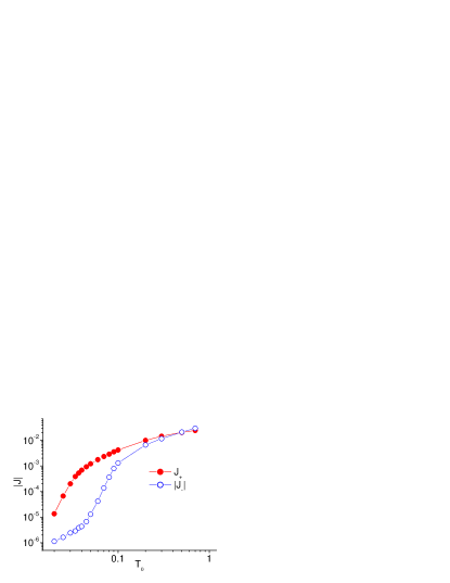
Figure 2: (Color Online) Heat current of the system with $N_{Y}=4$ and $N_{X}=10$ versus $T_{0}$. $|\Delta|$=0.5

The model we used is a simple extension from one dimension to two dimension, however the results in Fig2 show that it truly demonstrates good rectifying effect on heat current. In Fig 2, we can see the visible difference between $J_{+}$ and $J_{-}$ in very wide temperature range. The difference varies from few times to several hundreds times.

III Dependence of rectifying effect on temperature and temperature difference

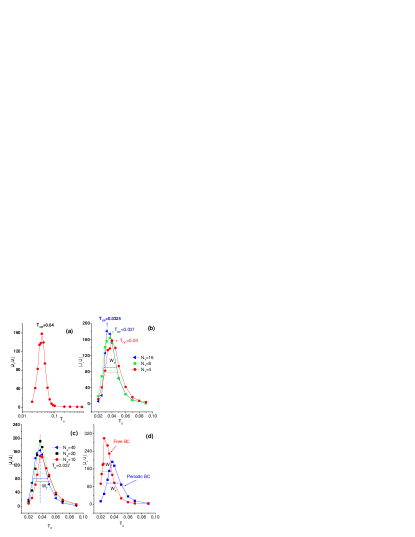
Figure 3: (Color Online) The rectifying efficiency, $|J_{+}/J_{-}|$, versus $T_{0}$ at different conditions. (a)The system with $N_{Y}=4$, $N_{X}=10$, and $|\Delta|=0.5$. $T_{OP}=0.04$. (b) Comparison for three different $N_{Y}$ with $N_{X}=40$. $T_{OP}=0.04$, $W_{T}=0.022$ and $\vartheta=0.55$ for the case of $N_{Y}=4$. When $N_{Y}=8$, $T_{OP}=0.037$, $W_{T}=0.022$ and $\vartheta=0.59$. When $N_{Y}=16$, $T_{OP}=0.0325$, $W_{T}=0.018$ and $\vartheta=0.55$.(c) Comparison for three different $N_{X}$ with $N_{Y}=8$. They have the same $T_{OP}=0.037$. When $N_{X}=10$, $W_{T}=0.023$ and $\vartheta=0.62$. When $N_{X}=20$, $W_{T}=0.020$ and $\vartheta=0.54$. When $N_{X}=40$, $W_{T}=0.022$ and $\vartheta=0.59$. (d) Comparison for different boundary conditions along $Y$ direction with $N_{Y}=8,N_{X}=20$. Free boundary: The optimum performance (OP)$OP=298.5$, $T_{OP}=0.025$, $W_{T}=0.014$, $\vartheta=0.56$; Periodic boundary: $OP=191.5$, $T_{OP}=0.037$, $W_{T}=0.022$, $\vartheta=0.59$.

In this section, we study the dependence of the system performance on the temperature change. Fig 3 shows the rectifying efficiency $|J_{+}/J_{-}|$ versus $T_{0}$. In Fig3(a), we can see that there exists an optimum performance (OP) of the rectifying effect when changing temperature $T_{0}$. We can define the temperature for the optimum performance as $T_{OP}$. In Fig3b, Fig3c and Fig3d we show the dependence of the ratio $|J_{+}/J_{-}|$ on temperature under different conditions. We found that $T_{OP}$ depends on the system settings along $Y$ direction. In Fig3b, the number of particles along $Y$ direction varies from 4 to 8 and 16 while other settings are kept unchanged. We can see clearly that $T_{OP}$ shifts to lower temperature when increasing $N_{Y}$. The value of $T_{OP}$ is 0.04, 0.037, 0.0325 for $N_{Y}=4$, 8 and 16, respectively. $T_{OP}$ keeps the same value when we change $N_{X}$. This is shown in Fig3c. In Fig3d, we change the periodic boundary condition in $Y$ direction to free boundary condition. $T_{OP}$ and the optimum performance change drastically. $T_{OP}$ changes from 0.037 to 0.025 and the ratio increases almost 100%.

Quantity $W_{T}$ in the figures is a parameter defined as the width of the effective temperature range $T_{e}$ over the half value of OP, while $\vartheta=W_{T}/T_{OP}$ is defined as the quality factor. $T_{e}$, $W_{T}$, and $\vartheta=W_{T}/T_{OP}$ are useful parameters to estimate the temperature range in which the system has a good rectifying effect. In our investigation, $T_{e}$ broadens from the center [0.03-0.46] to high temperature region or low temperature region. The typical value of $W_{T}$ under different settings is around 0.018-0.023. $\vartheta$ is always larger than 0.5. The results suggest that the system is effective in very wide temperature range.

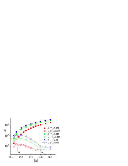
Figure 4: (Color Online) Heat current of the system with $N_{Y}=8,N_{X}=20$ versus temperature difference at three different $T_{0}$. Note that $|J_{-}|$ decreases as $|\Delta|$ increases in the interval $0.1<|\Delta|<0.6$, this is the so-called ”negative differential thermal resistance”, see context for more explanation.

In Fig4, we show the heat current versus the (normalized) temperature difference, $\Delta$, for three different $T_{0}$. Full symbols represent $J_{+}$ and empty ones $|J_{-}|$. We can see that $J_{+}$ increases with $\Delta$ monotonically and it always larger than $|J_{-}|$, while $J_{-}$ changes with $\Delta$ in different ways. One can find that there are three regions for $|J_{-}|$. In the first region, $|\Delta|<0.1$, the increase of $\Delta$ leads to the increase of the heat current. However, in the second region, $0.1<|\Delta|<0.6$, the increase of $|\Delta|$ does not induce the increase of $|J_{-}|$, instead it results in a decrease of $|J_{-}|$. In the third region, $\Delta>0.6$, $|J_{-}|$ is almost a constant independent of $|\Delta|$. In this region, the $|J_{-}|$ is so small that the system can be approximately considered as an insulator. The ratio $|J_{+}/J_{-}|$ becomes larger and larger when $|\Delta|$ increases. That indicates that rectifying effect increases with increasing temperature difference.

The strange behavior of $|J_{-}|$ observed in the second region, namely, the larger the temperature difference the smaller the heat current, is called negative differential thermal resistance. As we will demonstrate later that this is a typical phenomenon in nonlinear lattices. It can be understood from the match and mismatch of the vibrational spectra of the interface particles.

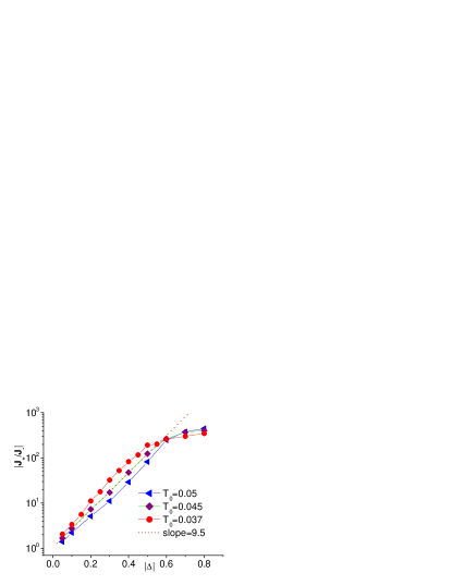
Figure 5: (Color Online) The ratio of heat current, $|J_{+}/J_{-}|$ versus half normalized temperature difference $|\Delta|$ at temperature $T_{0}=0.037,0.045,0.05$. The dotted line has a slope of 9.5.

Fig5 shows $|J_{+}/J_{-}|$ versus $|\Delta|$. It is found that $|J_{+}/J_{-}|$ increases with $|\Delta|$ in an exponential way in the regime in which $|\Delta|$ is smaller than $\Delta_{2}$. Approximately,

$$|J_{+}/J_{-}|\propto\exp(c*|\Delta|)+\delta,$$ (11)

here $c$ is about 9.5 under the particular parameter setting $N_{Y}=8$ and $N_{X}=20$ with periodic boundary condition along $Y$ direction. When we change $N_{Y}$, $N_{X}$ or boundary condition along $Y$ direction, $c$ changes slightly, but it is always around 10. The variation of $|c-10|$ is smaller than 0.5 in our investigation. $\delta$ is related with $T_{0}$ and $\Delta$.

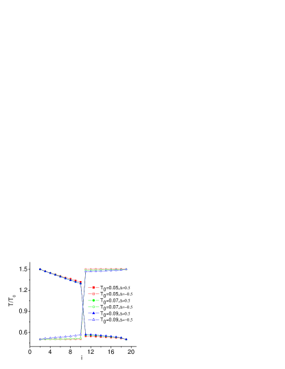
Figure 6: (Color Online) $T/T_{0}$ versus lattice site for $T_{0}$=0.05, 0.07, and 0.09. The solid symbols are for the cases of $\Delta=0.5$ and the empty symbols are for the cases of $\Delta=-0.5$. $N_{Y}=8,N_{X}=20$.

IV Interface Thermal Resistance (ITR) - Kapitza resistance

Thermal resistance between two different materials or between twin or twist boundaries of the same material has been extensively studied both experimentally and theoretically Kinder ; Nakayama ; Cahill ; Kapitza . In fact, the existence of a thermal boundary resistance between a solid and superfluid helium was first detected by KapitzaKapitza as early as 1940’s. This boundary resistance is named Kapitza resistance after him. Later, it is found that such a Kaptiza resistance exists at the interface between any pair of dissimilar materials. KhalatnikovKhalatnikov developed the acoustic mismatch model to explain the Kapitza resistance. Since then, continuous efforts have been devoted to this problem. More information can be found in the review by Swartz and Pohl SwartzPohl .

The Kapitza resistance is defined as

$$R=\Delta T/J,$$ (12)

where $J$ is the heat current and $\Delta T$ the temperature difference between two sides of the interface.

In our system, the temperature drops are different when the temperature gradient of the system is reversed as shown in Fig. 6. Therefore, we use $R_{+}$ and $R_{-}$ to denote the interface resistance for the case of $\Delta>0$ and $\Delta<0$, respectively.

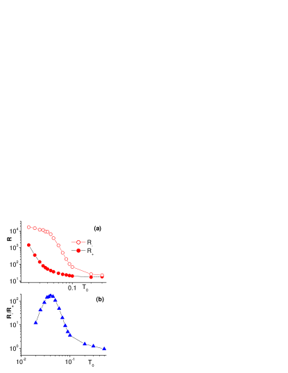
Figure 7: (Color Online) (a) Interface thermal resistance $R_{\pm}$ versus $T_{0}$. $|\Delta|=0.5$. (b) The ratio $R_{-}/R_{+}$ versus $T_{0}$. $N_{Y}=4,N_{X}=10$.

In Fig7 and Fig8, we show the dependence of IRT on temperature $T_{0}$ and the normalized temperature difference $\Delta$. From the two figures we can see that, generally, $R_{-}$ (with larger temperature drop) is about two or three orders of magnitude larger than $R_{+}$ (with smaller temperature jump). Both $R_{+}$ and $R_{-}$ decrease with $T_{0}$ until $T_{0}\approx 0.2$, then both become approximately constants. In Fig7b, we show the ratio $R_{-}/R_{+}$ versus temperature $T_{0}$. It is clearly seen that there exists an optimal temperature value for the ratio $R_{-}/R_{+}$. In Fig8, we show the resistance versus temperature difference. We can see that $R_{-}$ monotonically increases with temperature difference until it reaches a maximum value, while $R_{+}$ monotonically decreases with increasing $\Delta$. If we plot the ratio of $R_{-}$ over $R_{+}$ versus temperature difference, we find that the relationship between them also obeys the exponential law like the ratio of heat current.

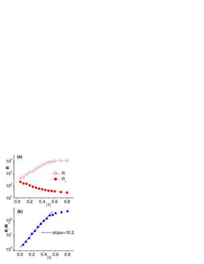
Figure 8: (Color Online) (a) $R_{\pm}$ versus the normalized temperature difference $|\Delta|$. $T_{0}=0.037$. (b) The ratio $R_{-}/R_{+}$ versus $|\Delta|$. $N_{Y}=8,N_{X}=20.$

Comparing Fig7 and Fig8 with Fig3 and Fig5, we can find that the behaviors of the IRT and heat current through the system is very similar, both are asymmetric, both the ratio $R_{-}/R_{+}$ and $J_{+}/J_{-}$ have an optimum value under different temperature and obey exponential law when changing temperature difference. The asymmetry of thermal resistance when reversing temperature gradient is the determinant factor for the rectifying effect on heat current of the system from the formula (12).

V Physical Mechanism of Rectifying Effect: An Analysis of Lattice Vibration Spectrum

From above investigation, we know that the asymmetric interface thermal resistance determines the asymmetry of heat current when reversing temperature gradient on the system, but what cause the asymmetrical behavior of the ITR? In this section, we will answer this question from a fundamental point of view: lattice vibration spectrum. Lattice vibration is responsible to heat transport in our model. An effective way to get the spectrum of lattice thermal vibration is the discrete faster Fourier transform (DFFT) for the lattice velocity William .

In our model, the vibration has two components, $v_{x}$ and $v_{y}$. We can use the theorem of equipartition of energy to simplify the numerical calculation. According to the equipartition theorem, the molecules in thermal equilibrium (here we have local thermal equilibrium) have the same average energy associated with each independent degree of freedom of their motion and that energy is $k_{B}T/2$. For our system, we have $m\langle\textbf{v}^{2}\rangle/2=k_{B}T$, $m\langle v_{x}^{2}\rangle/2=m\langle v_{y}^{2}\rangle/2=k_{B}T/2$.

In our calculation, $m=1$, $k_{B}=1$. So we have $\langle v_{x}^{2}\rangle=\langle v_{y}^{2}\rangle=T$. If we do the DFFT of $v_{x}$ and $v_{y}$ separately, we should have, $\sum_{i=0}^{L-1}|v_{x}(t)|^{2}=\Delta f*\sum_{j=0}^{L/2-1}2|P_{x}(j)|^{2}$ and $\sum_{i=0}^{L-1}|v_{y}(t)|^{2}=\Delta f*\sum_{j=0}^{L/2-1}2|P_{y}(j)|^{2}$. Here $P(f)$ is the Fourier transform of velocity $v(t)$. From the equipartition theorem, one has $\sum_{i=0}^{L-1}|v_{x}(t)|^{2}/L=\langle v_{x}^{2}\rangle$ and $\sum_{i=0}^{L-1}|v_{y}(t)|^{2}/L=\langle v_{y}^{2}\rangle$ From above analysis, we have $\Delta f\sum_{j=0}^{L/2-1}2|P_{x}(j)|^{2}/L=T,\quad\Delta f\sum_{j=0}^{L/2-1}2|P_{y}(j)|^{2}/L=T.$ The power spectra of vibration obtained from DFFT of $v_{x}$ and $v_{y}$ agree with the above formula very well (see Fig9). The integral of power spectra is exactly equal to the temporal average of $v_{x}^{2}$ and $v_{y}^{2}$ individually. There is a slight difference between $\langle v_{x}^{2}\rangle$ and $\langle v_{y}^{2}\rangle$. The difference might be caused by the number of sampled data or the different boundary conditions in $X,Y$ direction. In the formula, $L$ should be infinite.

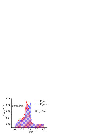
Figure 9: (Color Online) DFFT of $v_{x},v_{y}$. The shadowed regions represent the integral of the power spectra. $2S(P_{x}(\omega/2\pi)/L)=0.05=\langle v_{x}^{2}\rangle\approx T$,$2S(P_{y}(\omega/2\pi)/L)=0.05=\langle v_{y}^{2}\rangle\approx T$ .

In our system, we find that the asymmetrical ITR and heat current are strongly related with the overlap of vibration spectra of the particles at the two sides of the interface. When the vibration spectra overlap with each other, the system behaves like a thermal conductor, while the system behaves like a thermal insulator when the vibration spectra are separated.

Physically, whether an excitation of a given frequency can be transported through a mechanical system depends on whether the system has a corresponding eigenfrequency. If the frequency matches, the energy can easily go through the system, otherwise, the excitation will be reflected. In our system, the overlap of the two spectra means that there exists common vibrational frequency in two parts of the system. The excitation (here as phonon) of such common frequency can be transported from one part to the another. However, if the vibrational spectra of two parts are separated, then the excitation at any part cannot be transported to another part, because there exists no such corresponding frequency in another part.

The change from overlap to separation is induced by the different temperature dependence of the vibration spectra of the two segments, which is a general feature of any anharmonic lattice.

In Fig10, we show the vibration spectra of the FK part and the FPU part under different temperatures. We can see that the vibration spectra of the FK part broaden from high frequency to low frequency when increasing the system temperature. This is because at low temperature, the atoms of the FK model is confined at the valley of the on-site potential, thus the atoms oscillate in very high frequency, however, when the temperature is increased, more and more low frequency modes can be excited. In the limiting case, when the temperature is larger enough that the kinetic energy of the atom is much larger than the on-site potential, then the FK model becomes a chain of harmonic oscillators which has frequency $\omega\in[0,2\sqrt{k_{FK}}]$.

On the contrary, the vibration spectra of the FPU part broaden from low frequency to high frequency. In fact, we have shown Li05 that the highest oscillation frequency of the FPU model depends on temperature, $\omega_{FPU}\sim T^{1/4}$. Therefore, in some settings, the vibration spectra of the FK part and the FPU part will overlap with each other, while in other temperature settings, they will separate with each other. These are shown in Fig11. The comparison of vibration spectra of the FK part at two different temperature ranges and the FPU part at the full temperature range from 0.01 to 0.12 are shown in Fig11a and Fig11b separately. We can see that the vibration spectra of the FK part and the FPU part are matched with each other when the temperature of the FK part is from 0.05 to 0.12 (see Fig11a). The vibration spectra of the two parts are separated from each other when the temperature of the FK part is from 0.01 to 0.03 (see Fig11b). This indicates that when the temperature of the FK part is below a certain value, which we call $T_{c}$ ($0.04\sim 0.045$), the system will behave like a thermal insulator since the separated vibration spectra of the interface particles make the heat conduction almost impossible. When the temperature of the FK part is above the critical point $T_{c}$, the system will be a good thermal conductor since the matched vibration spectra allow the heat flow. Thus, if we adjust $T_{0}$ and $\Delta$ appropriately to make $T_{high}\geq T_{c}$ and $T_{low}\leq T_{c}$ , the system will have a good rectifying effect. If $T_{high},T_{low}>T_{c}$ or $T_{high},T_{low}<T_{c}$ , the rectifying effect is very poor. The above analysis is based on the vibration spectra of the system with $N_{Y}=8,N_{X}=20$. It is consistent with the result obtained in Section III.

Now we look back at Fig3. The optimum point is at $T_{0}=0.037$ for $N_{Y}=8,N_{X}=20$, corresponding $T_{high}=0.0505>T_{c}$ and $T_{low}=0.0235<T_{c}$. The effective temperature range $T_{e}$ with $|\Delta|=0.5$ is from 0.0261 to 0.0481. The low temperatures are all smaller than $T_{c}$ and all high temperatures are larger than $T_{c}$. Both decreasing $T_{0}$ and increasing $T_{0}$ in the outside region of $T_{e}$ lead the system to the two extreme cases $T_{high},T_{low}\geq T_{c}$ or $T_{high},T_{low}\leq T_{c}$ with poor performance. From the above analysis, we can say that the different properties of heat current under different temperature and temperature difference are determined by the temperature dependence of the vibration spectra of the two segments.

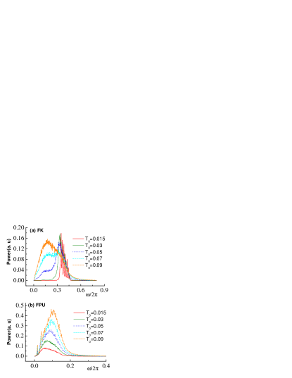
Figure 10: (Color Online) Vibration spectra of the interface particles at different temperature. (a) The vibration spectra of the particles in the FK segment.(b) The vibration spectra of the particles in the FPU segment.

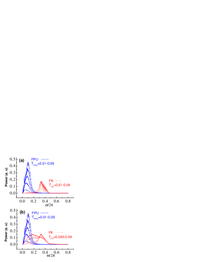
Figure 11: (Color Online) Comparison of the spectra of the FK part and the FPU part at different temperature region. (a) The spectra of the FPU part at $T_{FPU}=0.01-0.09$ (from bottom to top) and the FK part at $T_{FK}=0.01-0.04$ . (b) The spectra of the FPU part at $T_{FPU}=0.01-0.09$ and the FK part at $T_{FK}=0.045-0.09$

In terms of the vibration spectra of the particles in the interface, the complex behavior of $|J_{-}|$ in Fig 4 can be explained from the vibration spectrum. In particular, in the range from $\Delta_{1}$ to $\Delta_{2}$, a novel phenomenon- called the negative differential thermal resistance phenomenon is observed in Ref. BLi04 and fully discussed in Ref BLi05 . In this particular temperature interval, a larger temperature difference can induce a smaller heat current. The negative differential thermal resistance can be understood from the overlap and separation of the vibration spectra of the interface particles. This phenomenon is valid for a wide range of the parameters. Moreover, in Ref BLi05 , Li. et. al. show that it is this negative differential thermal resistance property that makes the thermal transistor possible.

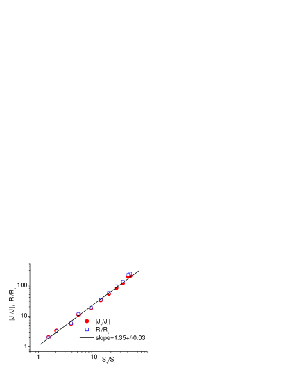
Figure 12: (Color Online) The bullet are the ratios of heat current $|J_{+}/J_{-}|$ versus $S_{+}/S_{-}$ . Square are the ratios of the ITR $R_{-}/R_{+}$ versus $S_{+}/S_{-}$. The dotted line has a slope $1.35\pm 0.03$.

More importantly, we find a specific relationship between the overlap of the vibration spectra of the two segments and the ratio $R_{-}/R_{+}$ in the interface or the ratio $|J_{+}/J_{-}|$ from two directions. We introduce the following quantity to describe overlap of the vibration spectra,

$$S_{\pm}=\frac{\int P^{x}_{l}(f)P^{x}_{r}(f)df}{\int P^{x}_{l}(f)df\int\\ P^{x}_{r}(f)df}=\frac{\int P^{x}_{l}(f)P^{x}_{r}(f)df}{T_{int}^{L}T_{int}^{R}}$$ (13)

$S_{\pm}$ corresponds to the case of $\Delta>0$ and $\Delta<0$, respectively. In Fig12, we plot $S_{+}/S_{-}$ versus $R_{-}/R_{+}$ and $|J_{+}/J_{-}|$. A very good power law was found between the ratio of resistances or heat currents and the overlap of the vibration spectra:$|J_{+}/J_{-}|\sim R_{-}/R_{+}\propto(S_{+}/S_{-})^{\gamma}$ The best fit for the ratio of current suggests the power law constant $\gamma=1.35\pm 0.03$. The two figures Fig11 and Fig12 give us a very clear and quantitative picture about the dependence of the rectifying effect of the system on the vibration spectra.

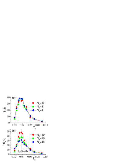
Figure 13: (Color Online) The ratio of the overlap of vibration spectra $S_{+}/S_{-}$ versus $T_{0}$ at different conditions. (a) Comparison at three different $N_{Y}$ with $N_{X}=20$.(b) Comparison at three different $N_{X}$ with $N_{Y}=8$.

Since the rectifying effect sensitively depends on the overlap of the vibration spectra, we may find answers in Fig13 for the behavior of the 2D system responding to the temperature changes at different conditions. We can see clearly that when we change the number of particles in $Y$ direction, the temperature for the optimum performance will change, whereas when we change the number of particles in $X$ direction, the temperature for OP are kept at the same value. And the value of the temperature for the OP at different conditions found by the overlap are consistent with the value in Fig3. These results suggest that the different vibration spectra of the two segments and the overlap between them are the determinant factors of the system complex behaviors.

VI Discussion and conclusions

In this paper, we have studied the thermal rectifying effect in a 2D anharmonic lattice. The performance of the 2D thermal rectifier under different environment changes, such as system temperature and the temperature difference on the two sides of the system, have been investigated systematically. We find that there exits an optimum performance (OP) for a specific thermal rectifier at certain temperature range. The OP is affected by the boundary condition and the number of particles, $N_{Y}$, along $Y$ direction. The OP shifts to lower temperature when increasing $N_{Y}$ or changing the periodic boundary condition to the free boundary condition along $Y$ direction. The 2D thermal rectifier has a good rectifying efficiency in a very wide temperature range. Another important factor that affects the performance of the thermal rectifier is the temperature difference between the two ends. We find the rectifying efficiency increases approximately as an exponential law in certain temperature range with the temperature difference. The rectifying efficiency is mainly determined by the asymmetrical ITR. The study on the ITR shows the similar behavior with heat current.

The behaviors of the ITR and heat current of the system are strongly correlated with vibration spectra of the particles beside the interface. The asymmetry behavior of ITR and heat current is induced by the different temperature dependence of the vibration spectra of the two parts beside the interface. We find the vibration spectra of the FK part broaden from high frequency to low frequency, conversely, the vibration spectra of the FPU part broaden from low frequency to high frequency as the temperature increases. The different temperature dependence of vibration spectra makes the system transition from a thermal conductor to an insulator possible by setting the system temperature and temperature difference properly. Moreover a specific relationship between the performance of the system and the convolution of the vibration spectra of the two parts is found numerically as power law.

Our study on 2D thermal rectifier gives a very clear picture about how the system responds to the environment changes. The results should be useful for further experimental investigation. The thermal diode constructed by a monolayer thin film or a tube like structure might have many practical applications.

VII Acknowledgement

We would like to thank Wang Lei for helpful discussions. This work is supported in part by a FRG of NUS and the DSTA under Project Agreement No. POD0410553.

References

- (1) R.E. Peierls, Quantum theory of solid (Oxford University Press, London, 1955).
- (2) G. Casati, J. Ford, F. Vivaldi, and W. M. Visscher, Phys. Rev. Lett. 52, 1861 (1984).
- (3) T. Prosen and M.Robnik, J. Phys. A 25, 3449(1992).
- (4) H. Kaburaki and M. Machida, Phys. Lett. A 181, 85 (1993).
- (5) S. Lepri, R. Livi and A. Politi, Phys. Rev. Lett. 78, 1896(1997).
- (6) S. Lepri, R. Livi and A. Politi, Europhys. Lett. 43, 271 (1998).
- (7) S. Lepri, Phys. Rev. E 58, 7165 (1998).
- (8) S. Lepri, R. Livi and A. Politi, Phys. Rep. 377, 1 (2003).
- (9) B. Hu, B. Li, and H. Zhao, Phys. Rev. E 57, 2992 (1998).
- (10) A. Fillipov, B. Hu, B. Li, and A. Zeltser, J. Phys. A 31,7719 (1998).
- (11) B. Hu, B. Li, and H. Zhao, Phys. Rev. E 61,3828 (2000).
- (12) F. Bonetto, J. L. Lebowitz, and L. Ray Bellet, et al., in Mathematical Physics 2000, edited by A. Fokas et al. (Imperial College Press, London, 2000), p.128;.
- (13) C. Giardiná, R. Livi, A Politi and M. Vasalli, Phys. Rev. Lett. 84, 2144 (2000)
- (14) O. V. Gendelman and A. V. Salvin, Phys. Rev. Lett. 84, 2381 (2000).
- (15) T. Prosen and D. K. Campbell, Phys. Rev. Lett. 84, 2857 (2000).
- (16) K. Aoki and D. Kusnezov, Phys. Rev. Lett. 86, 4029 (2001)
- (17) B. Li, L. Wang, and B. Hu, Phys. Rev. Lett. 88, 223901 (2002).
- (18) D. Alonso, A. Ruiz and I. de Vega, Phys. Rev. E 66, 066131 (2002).
- (19) B. Li, G. Casati, and J. Wang, Phys. Rev. E 67, 021204 (2003).
- (20) A. Pereverzev, Phys. Rev. E 68, 056124 (2003).
- (21) B. Li and J.Wang, Phys. Rev. Lett. 91, 044301 (2003).
- (22) B. Li, G. Casati, J.Wang, and T. Prosen, Phys. Rev. Lett. 92, 254301 (2004).
- (23) N.-B Li, P.-Q Tong, and B. Li, Europhys. Lett 75, 49 (2006).
- (24) M. Terraneo, M. Peyrard, and G. Casati, Phys. Rev. Lett. 88, 094302 (2002).
- (25) B. Li, L. Wang, and G. Casati, Phys. Rev. Lett.93, 184301 (2004).
- (26) B. Li, J Lan and L. Wang Phys. Rev. Lett. 95, 104302 (2005)
- (27) B. Hu and L. Yang, Chaos 15, 015119 (2005).
- (28) J.-S Wang and B Li, Phys. Rev. Lett 92, 074302 (2004), Phys. Rev. E 70, 021204 (2005).
- (29) S. Nośe, J. Chem. Phys. 81, 511 (1984); W. G. Hoover, Phys.Rev. A 31, 1695 (1985)
- (30) H. Kinder and K. Weiss, J. Phys.: Condens. Matter 5, 2063 (1993)
- (31) T. Nakayama, in Progress in Low Temperature Physics, edited by D. F. Brewer (North-Holland, Amsterdam, 1989), p. 115.
- (32) D. G. Cahill et al., J. Appl. Phys. 93, 793 (2003).
- (33) P. L. Kapitza, J. Phys. (Moscow) 4, 181 (1941).
- (34) I. M. Khalatnikov, Sov. Phys. JETP 22, 687 (1952).
- (35) E. T. Swartz and R. O. Pohl, Rev. Mod. Phys. 61, 605 (1989).
- (36) Numerical recipes, by H. P.William et al. Cambridge University Press 1986, 1992
- (37) B. Li, L. Wang and G. Casati, Appl. Phys. Lett, 88, 143501 (2006)