Unconventional Superconducting Symmetry in a Checkerboard Antiferromagnet

Abstract

We use a renormalized mean field theory to study the Gutzwiller projected BCS states of the extended Hubbard model in the large $U$ limit, or the $t$-$t^{\prime}$-$J$-$J^{\prime}$ model on a two-dimensional checkerboard lattice. At small $t^{\prime}/t$, the frustration due to the diagonal terms of $t^{\prime}$ and $J^{\prime}$ does not alter the $d_{x^{2}-y^{2}}$-wave pairing symmetry, and the negative (positive) $t^{\prime}/t$ enhances (suppresses) the pairing order parameter. At large $t^{\prime}/t$, the ground state has a $s-s$ wave symmetry. At the intermediate $t^{\prime}/t$, the ground state is $d+id$ or $d+is$-wave with time reversal symmetry broken.

I Introduction

Geometrically frustrated systems with strong correlation have attracted much attention due to the highly nontrivial interplay between frustration and correlation book ; Aoki . In such systems the pairwise interaction does not coincide with the geometry of the lattice, which may lead to exotic ground states. In particular, frustration in quantum magnets may cause certain types of magnetically disordered quantum phases, including the resonating valence bond (RVB) spin liquid state Anderson87 and the valence bond crystal state VBC . The quantum spin liquid state could become unconventional superconducting state when the charge carriers are introduced. There have been experimental evidences for the unconventional superconductors in these systems. Examples are the triangular layer cobaltates compound Na_xCoO₂ NaCoO , layered organic conductor $\kappa$-(ET)₂Cu₂(CN)₃ Org1 , the Kagome compound SrCr₈Ga₄O₁₉ Kagome , and 3-dimensional (3D) beta type transition-metal pyrochlore material KOs₂O₆ pyro1 ; pyro2 .

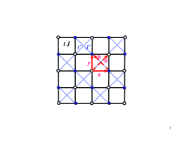
Figure 1: (Color online). Schematic structure of 2D checkerboard lattice. Solid (open) circles represent sublattice A (B). The hopping integral and spin-spin coupling are $t$ and $J$ for the nearest neighbor links (solid lines), and $t^{\prime}$ and $J^{\prime}$ for the diagonal or next nearest neighbor links (dashed lines), respectively.

To describe the interplay between frustration and correlation, we consider a $t$-$t^{\prime}$-$J$-$J^{\prime}$ model on a 2D checkerboard lattice, and analyze the possible superconducting pairing symmetry of the model. The checkerboard lattice is a frustrated one, and may be considered as a 2D projection of a 3D corner-sharing lattice of pyrochlore. A schematic checkerboard lattice is illustrated in Fig. 1. The Hamiltonian reads,

$$H= - \sum_{\langle ij\rangle\sigma}t_{ij}P_{D}(c_{i\sigma}^{\dagger}c_{j\sigma}+h.c.)P_{D}+\sum_{\langle ij\rangle}J_{ij}\vec{S}_{i}\cdot\vec{S}_{j}$$ (1)

$$- \mu\sum_{i\sigma}c_{i\sigma}^{\dagger}c_{i\sigma}$$

where $c_{i\sigma}^{\dagger}$ is an electron creation operator with spin $\sigma$ at site $i$, $\vec{S}_{i}$ is a spin operator for electron, $\mu$ is the chemical potential, and $\langle ij\rangle$ denotes a neighboring pair on the lattice. $P_{D}$ is a Gutzwiller projection operator to impose no double electron occupation at any site on the lattice. $t_{ij}$ and $J_{ij}$ stand for the hopping integrals and antiferromagnetic exchange couplings respectively, and $t_{ij}=t$, $J_{ij}=J$ for the nearest neighbor (n.n) links and $t_{ij}=t^{\prime}$, $J_{ij}=J^{\prime}$ for the diagonal or the next n.n. links as shown in Fig. 1. For convenience, we use $x,y$ to represent the n.n. links while $a,b$ to describe the two diagonal links. The Hamiltonian may be viewed as a strong coupling limit of a Hubbard model on the lattice with n.n. and next n.n. hopping integrals $t$ and $t^{\prime}$ respectively and a on-site Coulomb repulsive interaction $U$. Hereafter we use $t$ as an energy unit and set $J/t=1/3$. We choose $J^{\prime}/J=(t^{\prime}/t)^{2}$, consistent with the superexchange relation of $J=4t^{2}/U$ in the large $U$ limit of the Hubbard model.

The model has certain limiting cases. At $t^{\prime}/t\rightarrow 0$, the model is reduced to the $t$-$J$ model on a square lattice. At $t^{\prime}/t\rightarrow\infty$, the model becomes a collection of independent 1D $t^{\prime}$-$J^{\prime}$ chains. At $t^{\prime}/t=1$, it is an isotropic checkerboard lattice with a highly geometrically frustrated structure.

Previous theoretical investigations mainly focused on the half-filled case without charge carriers. A variety of techniques have been employed to study the quantum antiferromagetism on such a lattice Fuji ; paradigm ; olegt ; hermele ; Balents05 . Various quantum paramagnetic ground states may appear, which include some translational symmetry breaking states and a quantum spin liquid state. The introduction of doping with mobile charge carriers in a frustrated quantum antiferromagnet may result in the appearance of unconventional superconductivity Ogata03 ; d+id ; Kim04 ; palee ; Gan06 . Generally speaking, geometric frustration may play a key role in the mechanism of unconventional superconductivity. Recently exact diagonalization approaches have been employed to study the superconducting fluctuations in this system with $t^{\prime}$=$t$ and $J^{\prime}$=$J$ Poil1 ; Poil2 ; Poil3 . They found evidence of enhancement in pairing amplitude at arbitrarily small $J/t$ for a specific sign of the hopping amplitude.

In this paper, we apply the plain vanilla version of the RVB theory Zhang88 ; vannila to study the ground state of the $t$-$t^{\prime}$-$J$-$J^{\prime}$ model on a 2D checkerboard lattice. The competition among various superconducting states will be examined. Since our primary interest is on the possible pairing symmetry of the superconducting state for the doped system, we will not consider the possible long-range magnetic ordering in the present paper. Our main results can be summarized below. The $d_{x^{2}-y^{2}}$-wave pairing found for the $t$-$J$ model extends to a large region in parameter space of $t^{\prime}/t$ and doping concentration $\delta$, and the negative $t^{\prime}/t$ enhances the pairing while the positive $t^{\prime}/t$ suppresses the pairing. At small doping and for $|t^{\prime}/t|\sim 1$, there is a small region where the pairing symmetry is $d+id$ or $d+is$. At $|t^{\prime}/t|>1$, there are regions where the pairing symmetry belongs to a $s-s$ wave.

The rest of the paper is organized as follows. In Sec. II, we apply the renormalized mean field theory to study the RVB state. In Sec. III, we present our numerical results on the possible superconducting ground states. In particular, four distinct superconducting phases show up in the phase diagram as a function of $t^{\prime}/t$ and the doping $\delta$. Sec. IV is a summary. The diagonalization of the mean-field Hamiltonian and the explicit form of the self-consistent equations are presented in the Appendix.

II Formalism

We use a Gutzwiller projected BCS stateAnderson87 as a trial wavefunction to study the ground state and the corresponding pairing symmetry of the Hamiltonian (1). The trial wavefucntion is of the form,

$$|\Psi_{GS}\rangle=\prod\limits_{i}(1-n_{i\uparrow}n_{i\downarrow})|\Psi_{BCS}\rangle$$ (2)

where $n_{i,\sigma}=c^{{\dagger}}_{i,\sigma}c_{i,\sigma}$, and the projection operator $\prod\limits_{i}(1-n_{i\uparrow}n_{i\downarrow})$ removes the doubly occupied electron states on every lattice site $i$. We use a renormalized mean field theory  Zhang88 ; vannila to calculate the energy of the Hamiltonian (1). In the renormalized mean field theory, we adopt the Gutzwiller approximation to replace the projection by a set of renormalized factors, which are determined by statistical countings gutzwiller ; vallhardt . We have

$$\langle c_{i\sigma}^{\dagger}c_{j\sigma}\rangle=g_{t}\langle c_{i\sigma}^{\dagger}c_{j\sigma}\rangle_{0},~{}~{}~{}\langle\vec{S}_{i}\cdot\vec{S}_{j}\rangle=g_{s}\langle\vec{S}_{i}\cdot\vec{S}_{j}\rangle_{0}$$ (3)

where $g_{t}$ and $g_{s}$ are the Gutzwiller renormalized factors and are given by Zhang88 $g_{t}=2\delta/(1+\delta)$ and $g_{s}=4/(1+\delta)^{2}$ where $\delta$ denotes the doping density. Therefore, the variational calculations of $H$ of Eq. (1) in the projected BCS state is reduced to the variational calculations of an effective Hamiltonian $H_{eff}$ given below in the unprojected BCS states $|\Psi_{BCS}\rangle$ for $H_{eff}$ .

$$H_{eff} = \sum_{\langle ij\rangle\sigma}-g_{t}t_{ij}(c_{i\sigma}^{\dagger}c_{j\sigma}+h.c)+\sum_{(ij)}g_{s}J_{ij}\vec{S}_{i}\cdot\vec{S}_{j}$$ (4)

$$- \mu\sum_{i\sigma}n_{i\sigma}.$$

To proceed further, we introduce particle-particle and particle-hole mean fields, ($\tau=\pm\hat{x},\pm\hat{y},\pm\hat{a},\pm\hat{b}$, see Fig. 1)

$${\Delta}_{\tau} = \langle c^{{\dagger}}_{i\uparrow}c^{{\dagger}}_{i+\tau\downarrow}-c^{{\dagger}}_{i\downarrow}c^{{\dagger}}_{i+\tau\uparrow}\rangle_{0}$$

$$\xi_{\tau} = \sum_{\sigma}\langle c^{{\dagger}}_{i\sigma}c_{i+\tau,\sigma}\rangle_{0}.$$ (5)

Here we focus on the translational invariant state with the spin singlet and even parity superconducting pairing symmetry, where $\Delta_{i,i+\tau}=\Delta_{i+\tau,i}=\Delta_{\tau}$, and $\chi_{i,i+\tau}=\chi_{\tau}$. The superconducting order parameter is a $2\times 2$ matrix representing the two sublattices,

$$\Delta_{SC}(\vec{k})=\left(\begin{array}[]{cccc}\langle c_{\vec{k}\uparrow A}^{\dagger}c_{\vec{-k}\downarrow A}^{\dagger}\rangle&\langle c_{\vec{k}\uparrow A}^{\dagger}c_{\vec{-k}\downarrow B}^{\dagger}\rangle\\ \langle c_{\vec{k}\uparrow B}^{\dagger}c_{\vec{-k}\downarrow A}^{\dagger}\rangle&\langle c_{\vec{k}\uparrow B}^{\dagger}c_{\vec{-k}\downarrow B}^{\dagger}\rangle\\ \end{array}\right)$$ (8)

Within the Gutzwiller approximation, it is related to $\Delta_{\tau}$ by

$$\Delta_{SC}(\vec{k})=g_{t}\left(\begin{array}[]{cccc}\Delta_{a}cosk_{a}&\Delta_{x}cosk_{x}+\Delta_{y}cosk_{y}\\ \Delta_{x}cosk_{x}+\Delta_{y}cosk_{y}&\Delta_{b}cosk_{b}\\ \end{array}\right)$$ (11)

In the limit of $\delta=0$, consistent with the fact that the ground state is a Mott insulator at half filling. At small $\delta$, we have $\Delta_{SC}(\vec{k})\sim\delta$.

In terms of these mean fields, the effective Hamiltonian can be expressed as

$$H_{MF} = \sum_{\langle ij\rangle\sigma}-\frac{3}{8}g_{s}J_{ij}[\xi_{ij}c_{i\sigma}^{\dagger}c_{j\sigma}+\Delta_{ij}c_{i\sigma}c_{j\bar{\sigma}}+h.c.]$$ (12)

$$-g_{t}t_{ij}(c_{i\sigma}^{\dagger}c_{j\sigma}+h.c)-\mu\sum_{i\sigma}n_{i\sigma}+const.$$

There are eight independent complex mean-field parameters: $\xi_{x},\xi_{y},\Delta_{x},\Delta_{y}$ on the n.n. links and $\xi_{a},\xi_{b},\Delta_{a},\Delta_{b}$ on the next n.n. links. Here we assume all the particle-hole mean fields $\xi$ to be real. We denote $\theta_{x,y}$, $\theta_{a,b}$, and $\theta_{x,a}$ as the relative phases of $(\Delta_{x},\Delta_{y})$, $(\Delta_{a},\Delta_{b})$, and $(\Delta_{x},\Delta_{a})$, respectively. The energy per site can be expressed in terms of the mean fields and is given by

$$E_{gs} = -2g_{t}t(\xi_{x}+\xi_{y})-g_{t}t^{\prime}(\xi_{a}+\xi_{b})$$ (13)

$$-\frac{3}{8}g_{s}J(\xi_{x}^{2}+\xi_{y}^{2}+|\Delta_{x}|^{2}+|\Delta_{y}|^{2})$$

$$-\frac{3}{16}g_{s}J^{\prime}(\xi_{a}^{2}+\xi_{b}^{2}+|\Delta_{a}|^{2}+|\Delta_{b}|^{2}).$$

The mean field parameters $\xi$ and $\Delta$ and the chemical potential $\mu$ can be determined by solving the self-consistent Eq. (5) together with an equation for the hole density. The mean field state at zero temperature can be obtained by the diagonalization of $H_{MF}$. We then determine the lowest energy state for each set of parameters $t^{\prime}/t$ and $\delta$. The detailed formalism of the diagonalization of $H_{MF}$ and the self consistent equations can be found in Appendix. These equations can be solved numerically, and the results are given in the next section.

Figure 2: Phase diagram of $t$-$t^{\prime}$-$J$-$J^{\prime}$ model on a checkerboard lattice in parameter space of hole density $\delta$ and $t^{\prime}/t$ obtained by the renormalized mean field theory. The phases are indicated by their superconducting pairing symmetry defined in Table I, and $J^{\prime}/J=(t^{\prime}/t)^{2}$.

III Numerical Results

Table 1: The pairing symmetries (shown in Fig. 2 and used in the text) of the ground states of $t$-$t^{\prime}$-$J$-$J^{\prime}$ model on a checkerboard lattice and their corresponding mean fields $\Delta_{\tau}$ of Eq. (5). $\theta_{\tau,\tau^{\prime}}$ are the relative phase between $\Delta_{\tau^{\prime}}$ and $\Delta_{\tau}$

. Pairing symmetry mean field parameters $d$ $\Delta_{x}=-\Delta_{y}$ , $\Delta_{a}=\Delta_{b}=0$ $d+id$ $\Delta_{x}=-\Delta_{y}$, $\Delta_{a}=-\Delta_{b}$, $\theta_{x,a}\approx\pi/2$ $s-s$ $\Delta_{x}=\Delta_{y}$, $\Delta_{a}=\Delta_{b}$, $\theta_{x,a}=\pi$ $d+is$ $\Delta_{x}=-\Delta_{y}$, $\Delta_{a}=\Delta_{b}$, $\theta_{x,a}\approx\pi/2$

In this section, we present the numerical results of the self-consistent renormalized mean field theory for Hamiltonian Eq. (1) on the checkerboard lattice. We will first discuss the phase diagram, then provide detailed analyses of the mean field parameters as functions of $\delta$ for several typical values of $t^{\prime}/t$. The phase diagram is shown in Fig. 2. The ground state at $\delta=0$ is a Mott insulator. At finite doping, the ground state is a superconducting state, with four different types of pairing symmetry, as illustrated in Table 1. Here we classify the pairing symmetry in terms of the relative phases between $\Delta_{y}$ and $\Delta_{x}$, between $\Delta_{b}$ and $\Delta_{a}$, and between $\Delta_{a}$ and $\Delta_{x}$. Such a classification is consistent with the four-fold rotational symmetry in the Bravis lattice of the checkerboard structure.

At the limit $t^{\prime}$=$J^{\prime}$=0, the model is reduced to the $t$-$J$ model, and the ground state has a $d_{x^{2}-y^{2}}$ or $d$-wave symmetry Zhang88 ; kotliar at finite doping. This pairing state is robust against the next n.n. terms. As we can see from Fig. 2, the $d$-wave pairing symmetry of the ground state extends to a large region of both positive and negative values of $t^{\prime}/t$. In such state, $\Delta_{a}=\Delta_{b}=0$, but there is an additional self-energy term arising from the next n.n. spin coupling. There are nodal quasiparticles, whose position are determined by the crossing of the lines $\cos{k_{x}}=\cos{k_{y}}$ and the Fermi surface, similar to those obtained in the $t$-$J$ model. Note that the $d$-wave pairing has been previously found to be stable against the weak frustrations as studied by various authors Ogata03 ; d+id ; Gan06 on anisotropic triangular lattices. At large $|t^{\prime}/t|$, the ground state has a $s-s$ wave pairing symmetry with $\Delta_{x}=\Delta_{y}$ and $\Delta_{a}=\Delta_{b}$. In that state, the relative phase between $\Delta_{a}$ and $\Delta_{x}$ is $\pi$. Between the above two regions, there is a small parameter region around $|t^{\prime}/t|=1$, where the ground state has a $d+id$ pairing symmetry at small $\delta$, and a $d+is$ phase at larger $\delta$ for negative $t^{\prime}/t$. In both $d+id$ and $d+is$ states, the relative phases between $\Delta_{a}$ and $\Delta_{x}$ are close to $\pi/2$, and are weakly dependent of $\delta$, and the time reversal symmetry is spontaneously broken. We note that Hamiltonian (1) is asymmetric with respect to positive and negative values of $t^{\prime}/t$, which is reflected in our phase diagram. Similar to the case in the $t$-$J$ model, the particle-particle mean field amplitude $\Delta$ disappears at large $\delta$, and the ground state becomes a normal metal. The details of the phase boundaries between the superconducting and normal metallic states will be elaborated below. We also note that in the limit $|t^{\prime}/t|\rightarrow\infty$, the ground state becomes 1D-like.

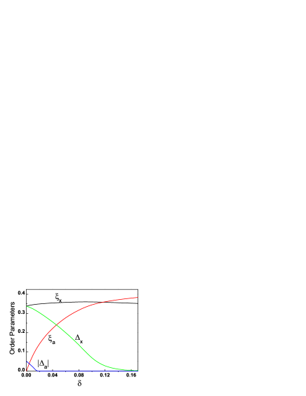
Figure 3: (Color online). Amplitudes of mean fields $\xi$ and $\Delta$ as functions of hole density $\delta$ for parameters $t=t^{\prime}=1,J=J^{\prime}=1/3$. The ground state has $d+id$ pairing (see Table 1) at $0<\delta<0.02$, and $d_{x^{-}y^{2}}$-wave pairing at $0.02<\delta<0.15$, and is a normal state at $\delta>0.15$.

In Fig. 3, we display the amplitudes of the mean field parameters as functions of $\delta$ at the symmetric point $t^{\prime}/t=1$. At very low hole density, the ground state has $d+id$-wave pairing symmetry, and $\Delta_{a}=i|\Delta_{a}|$, but $|\Delta_{a}|\ll\Delta_{x}$. As $\delta$ increases, the ground state becomes a $d$-wave, and $\Delta_{a}=\Delta_{b}$ vanishes. In comparison with the mean field amplitudes found in the $t$-$J$ model, $\xi_{x}$ is similar and insensitive to $\delta$, but $\Delta_{x}$ decreases more rapidly in the checkerboard model as $\delta$ increases. The latter may be understood as the consequence of the non-zero value of $\xi_{a}$ in the present case, which increases rapidly as $\delta$ increases. Note that the $s-s$ wave state has a very close energy, although it is slightly higher than either $d+id$- or $d$- wave states. Recently, Poilblanc Poil2 performed a finite cluster exact diagonalization study of the $t$-$J$ model on a checkerboard lattice. Some exotic states for positive $t$ are found to have $d_{x^{2}-y^{2}}$-, $s-s$- symmetries, which appears to be consistent with our results.

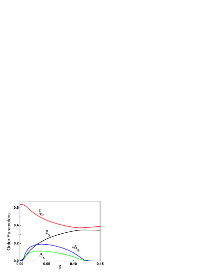
Figure 4: (Color online). Amplitudes of the mean fields $\xi$ and $\Delta$ as functions of $\delta$ for parameters $t=1,\,t^{\prime}/t=1.1,\,J=1/3,\,J^{\prime}/J=1.21$. The ground state is a $s-s$ wave at $0.02<\delta<0.12$, and a normal state otherwise.

The mean field amplitudes as functions of $\delta$ for the model at $t^{\prime}/t=1.1$ are depicted in Fig. 4. The ground state is a $s-s$ wave at $0.02<\delta<0.12$. The pairing amplitudes disappear around $\delta=0.12$, indicating the ground state to be a normal metallic state at $\delta>0.12$. As we can see, the correlations along the diagonal directions ($\hat{a}$ and $\hat{b}$) become more important than those along $\hat{x}$ and $\hat{y}$ directions at $t^{\prime}/t>1$. Note that the results near the half filled need to be cautious. At the half filling, the mean field ground state has only non-zero values of $\xi_{a}$ and $\xi_{b}$, indicating that the state is a collection of the decoupled chains along the directions of $\hat{a}$ and $\hat{b}$. This may attribute to the poor Gutzwiller approximation on 1D systemsZhang88 .

In Fig. 5 and Fig. 6, we show typical $\delta$ dependence of the mean field amplitudes for parameters $t^{\prime}/t<0$. In this case, $\xi_{a}$ and $\xi_{b}$ have the opposite sign with $\xi_{x}$ or $\xi_{y}$. At small value of $|t^{\prime}/t|$, the ground state is a $d$-wave state, the amplitudes of the mean fields are illustrated in Fig. 5 for $t^{\prime}/t=-0.5$. In that state, $\Delta_{a}=\Delta_{b}=0$, and $\xi_{a}=\xi_{b}$ are small and changes sign at $\delta>0.2$. Interestingly, $\Delta_{x}$ decreases much slower as $\delta$ increases, in comparison with that in the $t$-$J$ model. This suggests that the superconducting state may extend to a much larger hole density.

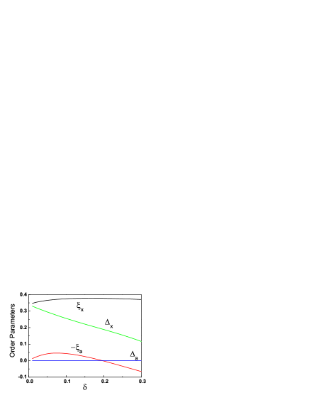
Figure 5: (Color online). Amplitudes of mean fields $\xi$ and $\Delta$ as functions $\delta$ in the case of $t=1,\,J=1/3,\,t^{\prime}/t=-0.5\,J^{\prime}/J=0.25$. $\Delta_{a}=\Delta_{b}=0$, and the ground state has a $d$-wave pairing symmetry(see Table 1).

In Fig. 6, we plot the mean field amplitudes for $t^{\prime}/t=-1$. Away from half-filling, the amplitudes of mean fields change nonmonotonically and there exist three distinct pairing symmetries with respect to different doping levels. As hole density increases, the ground state evolves from the $d+id$-wave state ($\Delta_{a}=-\Delta_{b}=i|\Delta_{a}|$) to the $d$-wave state and to $d+is$-wave state ($\Delta_{a}=\Delta_{b}=i|\Delta_{a}|$), as we can see from the figure that the amplitude of $\Delta_{a}$ decreases to zero around $\delta=0.02$ and arises again at $\delta=0.06$. In contrast to the $d+id$-wave state, the amplitude of $\Delta_{a(b)}$ is comparable to $\Delta_{x}$ in the $d+is$-wave state. In comparison with the case of positive $t^{\prime}/t$, we note that the suppression of $\Delta_{x}$ becomes much slower as $\delta$ increases and the superconductivity appears more favored for negative $t^{\prime}/t$. This result is in agreement with previous studies for a $t$-$J$ model on a triangular lattice Ogata03 ; d+id . An intuitive physical understanding of such effect can be given as follows: for positive $t^{\prime}/t$, the $t^{\prime}$ and $t$ terms in kinetic energy match quite well, so that $t^{\prime}$ term may enhance the kinetic energy (make it lower), hence suppress the pairing amplitude; for negative $t^{\prime}/t$, the $t^{\prime}$ term may introduce frustration in kinetic energy, hence enhances the pairing amplitude. The situation here is similar to that in cuprates, where the positive $t^{\prime}/t$ case corresponds to the electron-doped system while the negative $t^{\prime}/t$ case corresponds to the hole-doped system. It is well known that the hole-doped system has a higher transition temperature while the electron-doped system has a lower one and a substantial region in doping with antiferromagentic long range order which we have not considered in the present paper for simplicity.

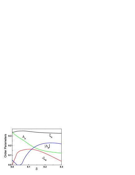
Figure 6: (Color online). Amplitudes of mean fields $\xi$ and $\Delta$ as functions $\delta$ for the parameters $t=1,\,J=J^{\prime}=1/3,\,t^{\prime}=-1$. The ground state is $d+id$-wave at $0<\delta<0.02$, $d$-wave at $0.02<\delta<0.06$, and $d+is$-wave at $\delta>0.06$.

IV Summary

We have applied the renormalized mean field theory to study the Gutzwiller projected BCS ground state for the $t$-$t^{\prime}$-$J$-$J^{\prime}$ model on a highly frustrated checkerboard lattice. As charge carriers are introduced, the half filled Mott insulator is evolved to resonating valence bond superconducting states, with four types of pairing symmetries depending on the hole density and the parameter $t^{\prime}/t$. We have found that the $d_{x^{2}-y^{2}}$ symmetry state previously obtained for the $t$-$J$ model is most stable in a large parameter region for small values of $|t^{\prime}/t|$. In this region, the $d$- wave pairing order parameter is suppressed for positive $t^{\prime}/t$ and enhanced for negative $t^{\prime}/t$. At large value of $|t^{\prime}/t|$, the ground state is found to be so-called $s-s$ wave. Around $|t^{\prime}/t|=1$, we have found the time reversal symmetry broken states. $d+id$- and $d+is$- symmetries states are the most stable. The appearance of the exotic superconducting pairing symmetry in the $t$-$t^{\prime}$-$J$-$J^{\prime}$ model on a checkerboard lattice may be viewed as the interplay between geometrically frustration and strong electron correlation. Our results may shed light on the understanding of the novel pairing symmetry features of highly frustrated systems.

HXH thanks X. Wan for numerical assistance. YC would like to thank Z.D. Wang and Q.H. Wang for helpful discussions. This research was supported by the RGC grants (HKU-3/05C, HKU7057/04P and HKU7012/06P) of Hong Kong SAR government, seed funding grant from the University of Hong Kong, and NSF in China No.10225419 and No.10674117.

V Appendix

In the appendix, we present detailed calculations of the mean field theory. We first diagonalize the mean field Hamiltonian (6) on the checkerboard lattice. We carry out the Fourier transformation of electron operator in the two sublattices $A$ and $B$,

$$c_{i\sigma}=\sum_{\vec{k}}\frac{1}{\sqrt{N}}a_{\vec{k}\sigma}\exp(i\vec{k}\cdot\vec{r}_{i}),\qquad i\in A$$ (14)

$$c_{i\sigma}=\sum_{\vec{k}}\frac{1}{\sqrt{N}}b_{\vec{k}\sigma}\exp(i\vec{k}\cdot\vec{r}_{i}),\qquad i\in B$$ (15)

The summation over $\vec{k}=(k_{x},k_{y})$ runs in the reduced Brillouin zone. $N$ is the number of sites in each sublattice. By using a spinor representation, the effective Hamiltonian can be written as

$$H_{eff}=\sum_{\vec{k}}\eta^{\dagger}_{\vec{k}}M_{\vec{k}}\eta_{\vec{k}}+const.,$$ (16)

where $\eta^{\dagger}_{\vec{k}}=(a^{\dagger}_{\vec{k}\uparrow},b^{\dagger}_{\vec{k}\uparrow},a_{-\vec{k}\downarrow},b_{-\vec{k}\downarrow})$ and the matrix $M_{\vec{k}}$ reads

$$M_{\vec{k}}=\left(\begin{array}[]{cccc}A(\vec{k})-\mu&B(\vec{k})\\ B^{\dagger}(\vec{k})&-A(\vec{k})+\mu\\ \end{array}\right)$$ (19)

where both $A(\vec{k})$ and $B(\vec{k})$ are $2\times 2$ matrices whose elements are given by

$$A_{11} = -(2g_{t}t^{\prime}+\frac{3}{4}g_{s}J^{\prime}\xi_{a})cos{k_{a}}$$

$$A_{22} = -(2g_{t}t^{\prime}+\frac{3}{4}g_{s}J^{\prime}\xi_{b})cos{k_{b}}$$

$$A_{12} = A_{21}=-2g_{t}t(cos{k_{x}}+cos{k_{y}})$$

$$-\frac{3}{4}g_{s}J(\xi_{x}cos{k_{x}}+\xi_{y}cos{k_{y}})$$

$$B_{11} = \frac{3}{4}g_{s}J^{\prime}\Delta_{a}\cos{k_{a}}$$

$$B_{22} = \frac{3}{4}g_{s}J^{\prime}\Delta_{b}\cos{k_{b}}$$

$$B_{12} = B_{21}=\frac{3}{4}g_{s}J(\Delta_{x}\cos{k_{x}}+\Delta_{y}\cos{k_{y}})$$

with $k_{\tau}=\vec{k}\cdot\vec{\tau}$. The matrix $M_{\vec{k}}$ can be diagonalized by employing an unitary transformation as

$$\left[{\begin{array}[]{*{20}c}{\gamma_{\vec{k}\uparrow}^{1{\dagger}}},&{\gamma_{\vec{k}\uparrow}^{2{\dagger}}},&{\gamma_{-\vec{k}\downarrow}^{1}},&{\gamma_{-\vec{k}\downarrow}^{2}}\\ \end{array}}\right]=$$ (21)

$$\left[{\begin{array}[]{*{20}c}{a^{\dagger}_{\vec{k}\uparrow}},&{b^{\dagger}_{\vec{k}\uparrow}},&{a_{-\vec{k}\downarrow}},&{b_{-\vec{k}\downarrow}}\\ \end{array}}\right]\left[{\begin{array}[]{*{20}c}{u_{1}^{1}}&{u_{1}^{2}}&{-v_{2}^{1*}}&{-v_{1}^{2*}}\\ {u_{2}^{1}}&{u_{2}^{2}}&{-v_{2}^{1*}}&{-v_{2}^{2*}}\\ {v_{1}^{1}}&{v_{1}^{2}}&{u_{1}^{1*}}&{u_{1}^{2*}}\\ {v_{2}^{1}}&{v_{2}^{2}}&{u_{2}^{1*}}&{u_{2}^{2*}}\\ \end{array}}\right]$$ (27)

where the $\vec{k}$ dependence of $u^{n}_{i}$ and $v^{n}_{i}$ are implied. The matrix element $u$ and $v$ satisfy the following conditions:

$$\begin{array}[]{l}\sum\limits_{i}{u_{i}^{1}}u_{i}^{2*}+v_{i}^{1}v_{i}^{2}=0\qquad\sum\limits_{i}{-u_{i}^{1}}v_{i}^{2}+v_{i}^{1}u_{i}^{2}=0\\ \sum\limits_{i}{u_{1}^{n}}u_{2}^{n*}+v_{1}^{n*}v_{2}^{n}=0\quad\sum\limits_{i}{u_{1}^{n}}v_{2}^{n*}-u_{1}^{n}v_{2}^{n}=0\end{array}$$ (30)

In terms of $u$’s and $v$’s the self-consistent equations for eight mean field and the hole density are given by,

$$\xi_{x(y)} = {2\over\textstyle N}\sum\limits_{k,n}{[fu_{1}^{n*}u_{2}^{n}+(1-f)v_{1}^{n}v_{2}^{n*}]\cos k_{x(y)}},$$

$$\xi_{a} = {2\over\textstyle N}\sum\limits_{k,n}{[f|u_{1}^{n}|^{2}+(1-f)|v_{1}^{n}|^{2}]\cos k_{a}},$$

$$\xi_{b} = {2\over\textstyle N}\sum\limits_{k,n}{[f|u_{2}^{n}|^{2}+(1-f)|v_{2}^{n}|^{2}]\cos(k_{b})},$$

$$\Delta_{x(y)} = {2\over\textstyle N}\sum\limits_{k,n}{[(1-f)u_{1}^{n}v_{2}^{n*}-fv_{1}^{n*}u_{2}^{n}]\cos k_{x(y)}},$$

$$\Delta_{a} = {2\over\textstyle N}\sum\limits_{k,n}{(1-2f)u_{1}^{n}v_{1}^{n*}\cos{k_{a}}},$$

$$\Delta_{b} = {2\over\textstyle N}\sum\limits_{k,n}{(1-2f)u_{2}^{n}v_{2}^{n*}\cos k_{b}},$$

$$1-\delta = {2\over\textstyle N}\sum\limits_{k,n}{f|u_{2}^{n}|^{2}+(1-f)|v_{2}^{n}|^{2}},$$

where the band index $n$ runs over $1,2$ and $f$ is the Fermi distribution function $f(E_{n})$ which is step function at zero temperature. The diagonalization of $M_{\vec{k}}$ and the self-consistent equations are carried out numerically to obtain the phase diagram and the results reported in the text.

References

• (1) H.T. Diep, Frustrated Spin Systems (World Scientific Publishing Co., Singapore, 2004).
• (2) H. Aoki, J. Phys. Cond. Matt. 16, V1 (2004).
• (3) P.W. Anderson, Science 235, 1196 (1987).
• (4) N. Read and S. Sachdev, Phys. Rev. Lett. 62 1694 (1989).
• (5) K. Takada, H. Sakurai, E. Takayama-Muromachi, F. Izumi, R.A. Dilanian and T. Sasaki, Nature 422, 53 (2003).
• (6) Y. Shimizu, K. Miyagawa, K. Kanoda, M. Maesato and G. Saito, Phys. Rev. Lett. 91, 107001 (2003).
• (7) P. Mendels, A. Keren, L. Limot, M. Mekata, G. Collin and M. Horvatic, Phys. Rev. Lett. 85, 3496 (2000).
• (8) S. Yonezawa, Y. Muraoka, Y. Matsushita and Z. Hiroi, J. Phys. Cond. Matt. 16, L9 (2004).
• (9) Y. Kasahara, Y. Shimono, T. Shibauchi, Y. Matsuda, S. Yonezawa, Y. Muraoka, and Z. Hiroi, Phys. Rev. Lett. 96, 247004 (2006).
• (10) S. Fujimoto, Phys. Rev. Lett. 89, 226402 (2002); Phys. Rev. B 67, 235102 (2003).
• (11) R.R.P. Singh, O.A. Starykh, and P.J. Freitas, J. Appl. Phys. 83, 7387 (1998).
• (12) O. Tchernyshyov, O.A. Starykh, R. Moessner, and A.G. Abanov, Phys. Rev. B 68, 144422 (2003).
• (13) M. Hermele, M.P.A. Fisher, and L. Balents, Phys. Rev. B 69, 064404 (2004).
• (14) O.A. Starykh, A. Furusaki, and Leon Balents, Phys. Rev. B 72, 094416 (2005).
• (15) M. Ogata, J. Phys. Soc. Jpn. 72, 1839 (2003).
• (16) B. Kumar and B.S. Shastry, Phys. Rev. B 68, 104508 (2003); G. Baskaran, Phys. Rev. Lett. 91, 097003 (2003).
• (17) C.H. Chung and Y.B. Kim, Phys. Rev. Lett. 93, 207004 (2004).
• (18) S.S Lee and P.A. Lee, Phys. Rev. Lett. 95, 036403 (2005).
• (19) J.Y. Gan, Y. Chen and F.C. Zhang, Phys. Rev. B 74, 094515 (2006).
• (20) A. Lauchli, D. Poilblanc, Phys. Rev. Lett. 92, 236404 (2004).
• (21) D. Poilblanc, Phys. Rev. Lett. 93, 197204 (2004).
• (22) D. Poilblanc, A. Lauchli, M. Mambrini, and F. Mila, Phys. Rev. B 73, 100403(R) (2006).
• (23) F.C. Zhang, C. Gros, T.M. Rice and H. Shiba, Supercond. Sci. Tech. 1, 36 (1988).
• (24) P.W. Anderson, P.A Lee, M. Randeria, T.M. Rice, N. Trivedi and F.C. Zhang, J. Phys. Cond. Matt. 24, R755 (2004).
• (25) M.C. Gutzwiller, Phys. Rev. 137, A1726(1965).
• (26) D. Vollhardt, Rev. Mod. Phys.56, 99 (1984).
• (27) G. Kotliar and J. Liu, Phys. Rev. B 38, 5142 (1988).