Level rearrangement in exotic atoms and quantum dots

Abstract

A presentation and a generalisation are given of the phenomenon of level rearrangement, which occurs when an attractive long-range potential is supplemented by a short-range attractive potential of increasing strength. This problem has been discovered in condensate-matter physics and has also been studied in the physics of exotic atoms. A similar phenomenon occurs in a situation inspired by quantum dots, where a short-range interaction is added to an harmonic confinement.

I Introduction

In 1959, Zel’dovich Zel59 discovered an interesting phenomenon while considering an excited electron in a semi-conductor. The model describing the electron–hole system consists of a Coulomb attraction modified at short-distance kolomeisky:022721 . A similar model is encountered in the physics of exotic atoms: if an electron is substituted by a negatively-charged hadron, this hadron feels both the Coulomb field and the strong interaction of the nucleus. The Zel’dovich effect has also been discussed for atoms in a strong magnetic field Karnakov .

Zel’dovich Zel59 and later Shapiro and his collaborators Kudryavtsev:1978af ; Shapiro:1978wi look at how the atomic spectrum evolves when the strength of the short-range interaction is increased, so that it becomes more and more attractive. The first surprise, when this problem is encountered, is that the atomic spectrum is almost unchanged even so the nuclear potential at short distance is much larger than the Coulomb one. When the strength of the short-range interaction reaches a critical value, the ground state of the system leaves suddenly the domain of typical atomic energies, to become a nuclear state, with large negative energy. The second surprise is that, simultaneously, the first radial excitation leaves the range of values very close to the pure Coulomb 2S energy and drops towards (but slightly above) the 1S energy. In other words, the “hole” left by the 1S atomic level becoming a nuclear state is immediately filled by the rapid fall of the 2S. Similarly, the 3S state replaces the 2S, etc. This is why the process is named “level rearrangement”. An illustration is given in Fig. 1, for a simple square well potential supplementing a Coulomb potential.

  

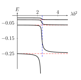
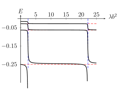
Figure 1: S-wave spectrum of the Coulomb potential (rescaled to $e^{2}=\hbar^{2}/(2\mu)=1$) modified by an attractive square well of radius $b=0.01$, and variable strength $\lambda$: first rearrangement (left) and second rearrangement (right). The dotted lines show the pure Coulomb energies and the coupling thresholds at which the square well alone supports one or two S-wave bound states.

In this article, the phenomenon of level rearrangement is reviewed and generalised, to account for cases where the narrow potential is located anywhere in a wide attractive well. An example is provided by a short-range pairwise interaction acting between two particles confined in an harmonic potential, a problem inspired by the physics of quantum dots. The basic quantum mechanics of exotic atoms will be briefly summarised, in particular with a discussion about the Deser–Trueman formula that gives the energy shift of exotic atoms in terms of the scattering length of the nuclear potential. A pedestrian derivation of this formula will be given in Appendix, which extents its validity beyond the case of exotic atoms. The link from the Coulomb to the harmonic cases will also be discussed in light of the famous Kustaanheimo–Stiefel (KS) transformation, which is reviewed in several papers (see, e.g., Mavromatis:1998 and refs. there) and finds here an interesting application.

The discussion is mainly devoted to one-dimensional problems or to S-states ($\ell=0$) in three dimensions. In Sec. VI, it is extended to the first P-state (2P), and it is shown that the rearrangement is much sharper for P and higher $\ell$ states than for S states.

II Coulomb potential plus short-range attraction

The simplest model of exotic atoms corresponds to the Hamiltonian

$$H=-\Delta-{1\over r}+\lambda v(r)~{},$$ (1)

where $v(r)$ has a range that is very short as compared to the Bohr radius of the pure Coulomb problem. Throughout this paper, the energy units are set such that $\hbar^{2}/(2\mu)=1$, where $\mu$ is the reduced mass. In (1) the scaling properties of the Coulomb interaction are also used to fix the elementary charge $e=1$, without loss of generality. The study will be restricted here to S-wave states. The case of P-states or higher waves is briefly discussed in Sec. VI.

As an example, a simple square well $v(r)=-\theta(b-r)$ is chosen in Fig. 1, with a radius $b=0.01$ which is small compared to the Bohr radius, which is $B=2$ in our units. If alone, this potential $\lambda v(r)$ requires a strength $\lambda_{n}b^{2}=(2n-1)^{2}\pi^{2}/4$ to support $n$ bound states in S-wave, with numerical values $\{\lambda_{n}b^{2}\}=\{2.46,22.2,\ldots\}$. These are precisely the values at which the atomic spectrum is rearranged in Fig. 1, with the $n$S state falling into the domain of nuclear energies and all other $i$S atomic states with $i>n$ experiencing a sudden change and drops to (but slightly above) the unperturbed $(i-1)$S energy.

The theory of level shifts of exotic atoms is rather well established, see e.g., (Ericson:1988gk, , Ch. 6). The discussion is restricted here to non-relativistic potentials, though exotic atoms have been more recently studied in the framework of effective field theory  Holstein:1999nq . Ordinary perturbation theory is not applicable here. For instance, a hard core of radius $b$ much smaller than the Bohr radius $B$ produces a tiny upward shift of the level, while first-order perturbation theory gives an infinite contribution! The expansion parameter here is not the strength of the potential, but the ratio $b/B$ of its range to the Bohr radius, and more precisely, the ratio $a/B$ of its scattering length to the Bohr radius. The scheme of this “radius perturbation theory” is outlined in Mandelzweig:1977cu . For the sake of this paper, the first order term of this new expansion is sufficient. It is due to Deser et al. Deser:1954vq , Trueman Trueman61 , etc., and reads

$${E_{n}-E_{0,n}\over E_{0,n}}\simeq-{4\over n}\left({a\over B}\right)~{},$$ (2)

where $a$ is the scattering length in the potential $\lambda v(r)$. Here, $E_{0,n}$ ($=-1/(4n^{2})$ in our units) is the pure Coulomb energy, and $E_{n}$ the energy of $n$S level of the modified Coulomb interaction ($n=1,2,\ldots$). Only in the case where $\lambda v(r)$ is very weak, the scattering length is given by the Born approximation, i.e., $a\propto\lambda$, and ordinary perturbation theory is recovered. A pedestrian derivation of (2) is given in Appendix A. The presence of $a$ instead of $\lambda$ in (2) indicates that the strong potential $\lambda v(r)$ acts many times, so that the shift is by no mean a perturbative effect.

The Deser–Trueman formula has sometimes been blamed for being inaccurate. In fact, if the scattering length is calculated with Coulomb interference effects, it is usually extremely good., see, e.g., Carbonell:1992wd for a discussion and Ericson:2003ju for higher-order corrections. However, this approximation obviously breaks down if the scattering length becomes very large, i.e., if the potential $\lambda v(r)$ approaches the situation of supporting a bound state.

Now the pattern in Fig. 1 can be read as follows. For small positive $\lambda$, the additional potential is deeply attractive but produces a small scattering length and hence a small energy shift. As the critical strength $\lambda=\lambda_{1}$ for binding in $\lambda v(r)$ is approached, the scattering length increases rapidly, and there is a sudden change of the energies. The ground-state of the system, which is an atomic 1S level for small $\lambda$ and a deeply bound nuclear state for $\lambda\gtrsim\lambda_{1}$ evolves continuously (from first principles it should be a concave function of $\lambda$, and monotonic if $v(r)<0$ Thirring:1979b3 ).

Beyond the critical region $\lambda\sim\lambda_{1}$, the scattering length $a$ becomes small again, but positive. Remarkably, the Deser–Trueman formula (2) is again valid, and accounts for the nearly horizontal plateau experienced by the second state near $E_{0,1}=-1/4$. A spectroscopic study near $\lambda\gtrsim\lambda_{1}$ would reveal a sequence of seemingly 1S, 2S, 3S, etc., states slightly shifted upwards though the Coulomb potential is modified by an attractive term. This is intimately connected with very low energy scattering: a negative phase-shift $\delta$ can be observed with an attractive potential which has a weakly-bound state, and mimics the effect of a repulsive potential. (The difference will manifest itself if energy increases: the phase-shift produced by a repulsive potential will evolve as $\delta(T)\to 0$ as the scattering energy $T$ increases, while for the attractive potential with a bound state, according to the Levinson theorem, $\delta(T)\to-\pi$.)

The occurrence of an atomic level near $E_{0,1}=-1/4$ for $\lambda\gtrsim\lambda_{1}$ can also be understood from the nodal structure. A deeply-bound nuclear state has a short spatial extension, of the order $b$. To ensure orthogonality with this nuclear state, the first atomic state should develop an oscillation at short distance, with a zero at $r_{0}\sim b/2$. This zero is nearly equivalent to the effect of a hard core of radius $r_{0}$. Hence, if $u(r)$ denotes the reduced radial wave function, the upper part of the spectrum evolves from the boundary condition $u(0)=0$ to $u(r_{0})=0$, a very small change if $r_{0}\ll B$.

As pointed out, e.g., in Refs. kolomeisky:022721 ; PhysRevC.26.2381 , the $\delta E_{n}\propto n^{-3}$ behaviour is equivalent to a constant “quantum defect”. For instance, the spectrum of peripheral S-waves excitations of Rydberg atoms is usually written as

$$E_{n}=-{\hbar^{2}\over 2\mu B^{2}}\,{1\over(n-\nu)^{2}}~{},$$ (3)

where $B$ is the Bohr radius, $\mu$ the reduced mass, and $\nu$ defines the quantum defect. A constant $\nu$ is equivalent to $\delta E_{n}\propto n^{-3}$, as for the Trueman formula (2). Indeed, if the excitation of the inner electron core is neglected, the dynamics is dominated by the Coulomb potential $-1/r$ felt by the last electron, which becomes stronger than $-1/r$ when this electron penetrates the core. Within this model, one can vary the strength of this additional attraction from zero to its actual value, or even higher, and it has been claimed that the Zel’dovich effect can be observed in this way, especially at high $n$ kolomeisky:022721 .

III The limit of a point interaction

The simplest solvable model of exotic atoms is realised with a zero-range interaction. The formalism of the so-called “point-interaction” is well documented, see, e.g., alb , where the case of a point-interaction supplementing the Coulomb potential is also treated, without, however, a detailed discussion of the resulting spectrum.

It is known that an attractive delta function leads to a collapse in the Schrödinger equation. In more rigorous terms, the Hamiltonian should be redefined to be self-adjoint. For S-wave, a point interaction of strength $g=1/a$, located at $r=0$, changes the usual boundary conditions $u(0)=0$, $u^{\prime}(0)=1$ (possibly modified by the normalisation) by $u^{\prime}/u=1/a$ at $r=0$. Note that $a$ is the Coulomb-corrected scattering length.

In this model, the S-wave eigenenergies are given by $u^{\prime}(0)/u(0)=1/a$ applied to the reduced radial wave function of the pure Coulomb problem, which results into alb

$$F(-2/k)=1/a~{},\quad F(x)=\Psi(1+x)-{1\over 2}\ln(x^{2})-{1\over 2x}~{},$$ (4)

in terms of the digamma function $\Psi(x)=\Gamma^{\prime}(x)/\Gamma(x)$. Using the reflection formula Abramovitz64 , the function $F$ can be rewritten as

$$F(-x)=\pi\cot(\pi x)+\Psi(x)-{1\over 2}\ln(x^{2})+{1\over 2x}~{},$$ (5)

explaining the behaviour observed on the left-hand side of Fig. 2.

Figure 2: Graph of the function $F$ used to calculate the spectrum for a Coulomb potential supplemented by a point interaction.

Equation (4) shows that $a\to-\infty$ corresponds to the plain Coulomb interaction, where $E_{n}=E_{0,n}$. For small deviations, the Trueman formula (2) can be recovered form Eq. (4), as shown in alb . The behaviour of the first $n$S levels is displayed in Fig. 3, for $a$ increasing from this limit: a sharp changes is clearly seen near $1/a=0$, beautifully illustrating the Zel’dovich effect.

Figure 3: First few energy levels in a Coulomb potential modified by a point interaction of strength $g$. The dotted lines correspond to the pure Coulomb levels $E_{0,n}$.

A comprehensive analytic treatment of the Zel’dovich effect has been given by Kok et al. PhysRevC.26.2381 using a delta-shell interaction $v(r)\propto-\delta(r-R)$, both for S-waves and higher waves ($\ell>0$).

IV Rearrangement with square wells

IV.1 Model

The patterns of energy shifts experienced by exotic atoms when the strength of nuclear potential increases can be studied in a simplified model where the three-dimensional Coulomb interaction is replaced by a one-dimensional square well supplemented by a narrow square well in the middle: the odd-state sector has the same type of rearrangement as the exotic atoms, while the even sector shows a new type of rearrangement. The effect of symmetry breaking can be studied by moving the attractive spike aside from the middle.

The potential, shown in Fig. 4, reads

$$V(x)=-V_{1}\theta(R_{1}^{2}-x^{2})-V_{2}\,\theta(R_{2}^{2}-x^{2})~{},$$ (6)

with value $-V_{1}-V_{2}$ for $0<|x|<R_{1}$, and $-V_{2}$ for $R_{1}<|x|<R_{2}$ and 0 for $|x|>R_{2}$, see Fig. 4. Slightly simpler would be the case of an infinite square well in which an additional well is digged: it can be proposed as an exercise.

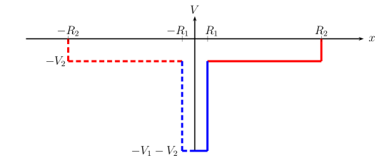
Figure 4: One-dimensional double square-well

The starting point $V_{1}=0$ with the model (6) is an one-dimensional square well of depth $V_{2}$ and radius $R_{2}$. Its intrinsic spectral properties depends only on the product $R_{2}^{2}V_{2}$. With a value 80, which is realised in the following examples with $R_{2}=1$ and $V_{2}=80$, there are six bound states, three even levels and three odd ones. See, e.g., bonfim:43 for solving the square well problem.

IV.2 Odd states in a symmetric double well

Besides a normalisation factor $\sqrt{2}$, the odd sector is equivalent to the S-wave sector in a central potential $V(r)$. The radial wave function $u(r)$ is thus $u(r)=u_{1}(r)=\sin(r\sqrt{V_{1}-k^{2}})$ for $r<R_{1}$, and $u(r)=u_{2}(r)=u_{1}(R_{1})\cos[k^{\prime}(r-R_{1})]+u^{\prime}_{1}(R_{1})\sin[k^{\prime}(r-R_{1})]/k^{\prime}$ if $R_{1}<r<R_{2}$ with $k^{\prime 2}=V_{2}-k^{2}$, and suitable changes $\sin\to\sinh$ and $\cos\to\cosh$ if $k^{2}>V_{2}$. The eigenenergies can be obtained by matching this intermediate solution $u_{2}$ to the external solution $u_{3}(r)=\exp(-kr)$ at $r=R_{2}$ , i.e., imposing $u_{2}(R_{2})u^{\prime}_{3}(R_{2})-u^{\prime}_{2}(R_{2})u_{3}(R_{2})=0$. The calculation involves only elementary trigonometric functions, and the spectrum can be computed easily.

The energy levels as functions of $V_{1}$ are displayed in Fig. 5. The rearrangement pattern is clearly seen, and is especially pronounced if $R_{1}\ll R_{2}$. The difference from the Coulomb case is that, for the square well, when a bound state collapses from the “atomic” to the “nuclear” energy range, a new state is created from the continuum.

   

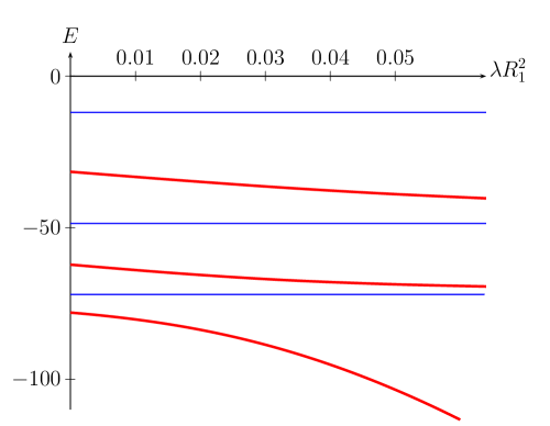
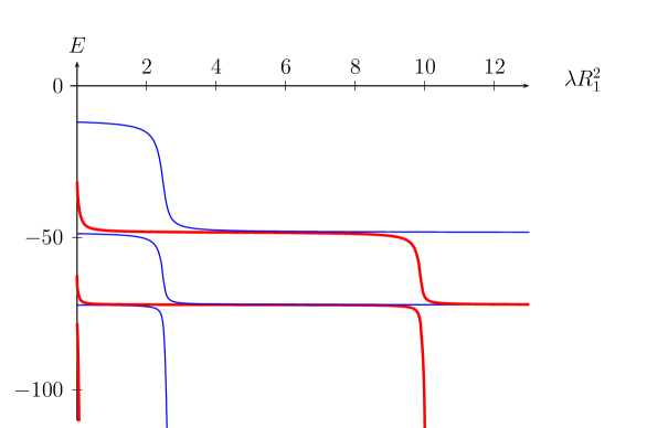
Figure 5: Level rearrangement of the odd (thin line) and even (thick line) states of the double square-well, with $R_{2}=1$, $V_{2}=80$, $R_{1}=0.01$ and increasing $V_{1}$.

IV.3 Even states in a double well

The even spectrum of the potential (6) is given by $w(x)=w_{1}(x)=\cos(x\sqrt{V_{1}-k^{2}})$ for $0\leq x<R_{1}$, and $w(x)=w_{2}(x)=w_{1}(R_{1})\cos[k^{\prime}(x-R_{1})]+w^{\prime}_{1}(R_{1})\sin[k^{\prime}(x-R_{1})]/k^{\prime}$ if $R_{1}<x<R_{2}$ with $k^{\prime 2}=V_{2}-k^{2}$, and suitable changes $\sin\to\sinh$ and $\cos\to\cosh$ if $k^{2}>V_{2}$. Then the matching to $w(x)=w_{3}(x)=\exp(-kx)$ gives the eigenenergies.

The results are shown in Fig. 5, with the same parameters as for the odd part. The same pattern of “plateaux” is seen as for the odd parts, with, however, some noticeable differences:

• In quantum mechanics with space dimension $d=1$ (actually for any $d\leq 2$), any attractive potential supports at least one bound state. In particular, a nuclear state develops in the narrow potential of width $2R_{1}$ even for arbitrarily small values of its depth $V_{1}$. Hence the ground-state level starts immediately falling down as $V_{1}$ increases from zero,

• The first even excitation does not stabilise near the value of the unperturbed even ground state, it reaches a plateau corresponding to the first unperturbed odd state.

• Similarly, each higher even level acquires an energy corresponding to the neighbouring unperturbed odd level.

• When $V_{1}R_{1}^{2}$ reaches about 2.46, enabling the narrow square well to support a second state, a new rearrangement is observed, with, again, values close to these of the unperturbed odd spectrum.

In short, the energies corresponding to the even states of the initial spectrum quickly disappear. The energies corresponding to the odd states remain, and become almost degenerate, except when a rearrangement occurs.

The degeneracy observed in Fig. 5 depends crucially on the addtional potential being of very short range. For comparison the case of a wider range $R_{1}=0.1$ is shown in Fig. 6. Though the rearrangement pattern is clearly visible, the transition is much smoother, and the almost degeneracy limited to smaller intervals of the coupling constant $V_{1}$, and less pronounced.

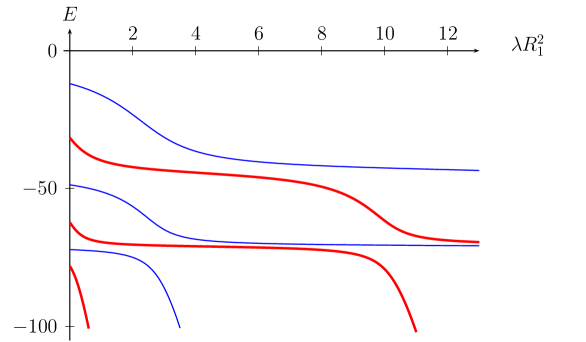
Figure 6: Same as Fig. 5, but for a wider range $R_{1}=0.1$ for the additional potential.

IV.4 Spectrum in an asymmetric potential

To check the interpretation of the patterns observed for the odd and even parts of the spectrum, let us break parity and consider the asymmetric double well of Fig. 7. For the sake of illustration, the centre of the spike is taken at $R_{0}=0.1$. The spectrum, as a function of $V_{1}$, is displayed in Fig. 8: Plateaux are observed, again, with energy values corresponding approximately to the combination of $(i)$ the spectrum in a well of depth $-V_{2}$ between $x=R_{0}+R_{1}$ and $x=R_{2}$ and a hard core on the left, i.e., a boundary condition $w(R_{0}+R_{1})=0$, and $(ii)$ the spectrum in a well of depth $-V_{2}$ between $x=-R_{2}$ and $x=R_{0}-R_{1}$ with $w(R_{0}-R_{1})=0$.

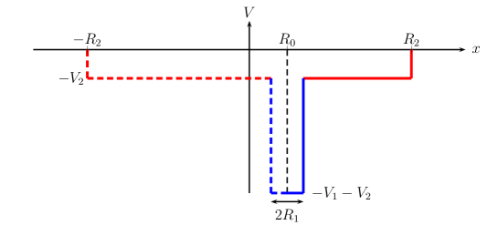
Figure 7: Asymmetric double square-well

   

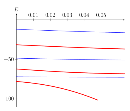
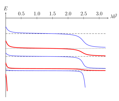
Figure 8: Spectrum in the asymmetric double square-well of Fig. 7, with $R_{2}=1$, $V_{2}=50$, $R_{1}=0.01$, $R_{0}=0.1$ and variable $V_{1}$. The dotted lines correspond to the states in the box $[-R_{2},R_{0}]$, and the dashed ones to those in the box $[R_{0},R_{2}]$, all with depth $V_{2}$ and hard wall at $R_{0}$.

It is interesting to follow how the wave function evolves when a rearrangement occurs. In Fig. 9, the third level is chosen. For $V_{1}=0$, it is the first even excitation with energy $E_{3}\simeq-62.18$, and the wave function $u(x)$ is the usual sinus function matching exponential tails. On the first plateau, with energy near $-70$, this wave function is almost entirely located on the right. As rearrangement takes place, the probability is shared by both sides. On the second plateau, with a energy near $-73$ corresponding to the ground state in the wider part with hard wall at $R_{0}$, the wave function is mostly on the left.

   

   

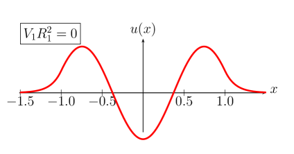
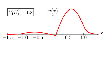
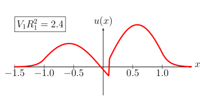
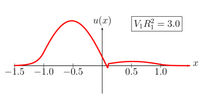
Figure 9: Wave function of the third level in the asymmetric double square-well of Fig. 7, with $R_{2}=1$, $V_{2}=80$, $R_{1}=0.01$, $R_{0}=0.1$ and variable $V_{1}$ near a rearrangement. An enlargement of the region near $x=0.1$ would confirm that the wave function and its derivative are continuous.

When the narrow well has only deeply bound states, it acts as an effective hard wall between the two boxes, at the right and and the left of $R_{0}$. However, when a new state occurs with a small energy and an extended wave function, it opens the gate, and states can move from the right to the left, or vice-versa.

It is possible to study how the spectrum in Fig. 8 evolves if the centre of the spike moves to the right, i.e., $R_{0}\to R_{2}-R_{1}$: the dotted line move up and disappear, while the dashed lines move down and become more numerous. Eventually, if the depth $V_{1}$ is large, the spectrum becomes very similar to the odd part of the spectrum in Figs. 4, 5, except for a change $R_{1}\to 2R_{1}$ and $R_{2}\to 2R_{2}$.; This illustrates again that for the upper part of the spectrum, a deep hole is equivalent to a hard wall.

V Rearrangement in quantum dots

V.1 Level rearrangement in an harmonic well

There is a considerable recent literature on quantum dots 0034-4885-64-6-201 , usually dealing with many particles in a trap, with a magnetic field. Let us consider the simplified problem of two particles confined by a wide harmonic trap, and interacting with short-range forces,

$$H={\boldsymbol{p}_{1}^{2}\over 2m}+{\boldsymbol{p}_{2}^{2}\over 2m}+Kr_{1}^{2}+Kr_{2}^{2}+\lambda v(|\boldsymbol{r}_{2}-\boldsymbol{r}_{1}|)~{}.$$ (7)

The centre-of-mass oscillates in a pure harmonic potential, and the separation $\boldsymbol{r}=\boldsymbol{r}_{2}-\boldsymbol{r}_{1}$ is governed by

$$h={\boldsymbol{p}^{2}\over m}+Kr^{2}+\lambda v(r)~{},$$ (8)

If $v(r)$ is attractive or, at least, has attractive parts, $\lambda v(r)$ will support bound states for large enough $\lambda$. The same phenomenon of level rearrangement is observed, as shown in the simple example of harmonic oscillator and square well. As for the case of exotic atoms, the effect of “level repulsion” is observed, that ovoids any crossing of trajectories corresponding to the same orbital momentum.

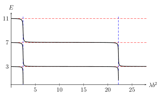
Figure 10: First few S-wave energy levels for an harmonic oscillator supplemented by a square well of variable strength, i.e., $V(r)=r^{2}-\lambda\Theta(b-r)$ and radius $b=0.01$. The vertical lines correspond to the coupling $\lambda_{1}=\pi^{2}/4$ and $\lambda_{2}=9\lambda_{1}$ at which a first and a second S-wave bound state occurs in the square well alone.

V.2 Dependence upon the radial number

As for the theory, it is similar to that of exotic atoms. The analogue of the Trueman–Deser formula, for any long-range potential combined with a short-rangfe potential, reads

$$\delta E_{n}\simeq 4\pi a\,|\phi_{n}(0)|^{2}~{},$$ (9)

indicating that the energy shift is proportional to the square of the value at the origin of the wave function of the pure long-range potential. It is worth pointing that the dependence upon the radial number $n$ is different for the Coulomb and the oscillator problems:

• For a narrow pocket of attraction added to an harmonic confinement, the energy shifts at large $n$ increase as $n^{1/2}$, since the square of the wave function at the origin is $|\phi_{n}(0)|^{2}=8/[\sqrt{\pi}B(n+1,1/2)]$, where $B$ is the beta function. But for very arge enough $n$, the first nodes of the radial function come in the range of $v(r)$, and then $\delta E$ decreases with $n$. Moreover, for very large $n$, the radial Schrödinger equation is dominated at short distance by the energy term.

• For a Coulomb interaction, $|\phi_{n}(0)|^{2}\propto n^{-3}$, and hence $\delta E_{n}\propto n^{-3}$, a well-known property of exotic atoms. As explained, e.g., in a review article on protonium Klempt:2002ap and briefly explained in Appendix, the first node of the $n$S radial function, as $n$ increases, does not go to $0$. In the case $\hbar^{2}/(2\mu)=e^{2}=1$, the node of the 2S level is at $r=4$, while the first node of $n$S at large $n$ is at $r\simeq 3.67$. Hence the Coulomb wave function never exhibits nodes within the range of the nuclear potential. Moreover, the energy term is always negligible in comparison with $\lambda v(r)$ at short distances.

V.3 From Coulomb to harmonic rearrangement

The KS transformation Mavromatis:1998 relates Coulomb and harmonic-oscillator potentials. The radial equation for a Coulomb system in three dimension (with $\hbar=2\mu=1$) reads

$$-u^{\prime\prime}(r)+{\ell(\ell+1)\over r^{2}}u(r)-{\alpha\over r}u(r)-Eu(r)=0~{},$$ (10)

with $u(0)=0$ and $u(r)\to 0$ as $r\to\infty$ becomes

$$-\phi^{\prime\prime}(\rho)+{L(L+1)\over\rho^{2}}\phi(\rho)+4(-E)\rho^{2}\phi(\rho)-4\alpha\phi(\rho)=0~{},$$ (11)

if $r=\rho^{2}$, $u(r)=\rho^{1/2}\phi(\rho)$, and $L=2\ell+1/2$. The modified angular momentum can be interpreted as relevant in a higher-dimensional world Mavromatis:1998 . But Eq. (11) is precisely the Schrödinger equation for the three-dimensional oscillator with (fixed) energy $4\alpha$ and oscillator strength $4(-E)$ (which is positive), i.e.,

$$4\alpha=\sqrt{-4E}(3+4n+2L)~{},\quad n=0,\,1,\ldots~{},$$ (12)

which is equivalent to the Bohr formula

$$E=-{\alpha^{2}\over 4(1+n+\ell)^{2}}~{},$$ (13)

where $1+n+\ell$ is the usual principal quantum number of atomic physics.

Now, an additional potential $\lambda v(r)$ in the Coulomb equation results into a short-range term $4\lambda\rho^{2}v(\rho^{2})$ added to the harmonic oscillator, and all results obtained for exotic atoms translate into the properties listed for a narrow hole added to an harmonic well.

Note that the $n$ dependence is also explained. In the KS transformation, the energy $E$ ($E<0$) in the Coulomb system becomes the strength $-4E$ of the oscillator, while four times the fine structure constant, i.e., $4\alpha$ ($\alpha>0$ for attraction) becomes the energy eigenvalue of the oscillator with angular momentum $L$. If $n$ increases, the oscillator deduced from the KS transformation becomes looser, and hence less sensitive to the short range attraction $4\lambda\rho^{2}v(\rho^{2})$. To maintain a fixed oscillator strength, one should imagine a different Coulomb system for each $n$, with $\alpha\propto n$, hence a Bohr radius independent of $n$, and a wave function at the origin $|\phi(0)|^{2}\propto n^{-1}$ instead of $n^{-3}$ in the usual case. Then, in this situation, $\delta E\propto n^{-1}$ for the Coulomb system, and $\delta\epsilon\propto n^{1/2}$ for the harmonic oscillator.

VI Rearrangement and level ordering

In the above examples, there is an interesting superposition of potentials with different level-ordering properties. A square well potential, if deep enough to support many bound states, has the ordering Landau

$$1S<2P<3D<2S<\ldots~{}.$$ (14)

We are adopting here the same notation as in atomic physics is adopted, i.e., 2P is the first P-state, 3D the first D-state, etc. The Coulomb potential, on the other hand, exhibits the well-known degeneracy

$$1S<2S=2P<3S=3P=3D<\ldots~{},$$ (15)

while for the harmonic-oscillator case,

$$1S<2P<2S=3D<\ldots~{},$$ (16)

with equal spacing.

The pattern of 1S, 2S and 2P levels for Coulomb (left) or harmonic oscillator (right) supplemented by a short-range square well of increasing strength is given in Fig. 11.

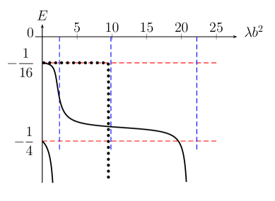
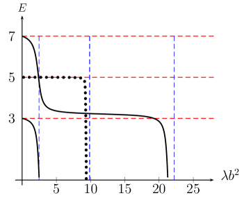
Figure 11: 1S and 2S levels (solid line) and 2P level (dotted line), for Coulomb (left) or harmonic-oscillator (right) potential plus a square well of radius $b=0.1$ of increasing strength $\lambda$. The horizontal lines are the unperturbed values, the vertical ones indicate the strength $\lambda$ at which the square well alone starts supporting a new bound state.

In the Coulomb case, the degeneracy is broken at small $\lambda$ as $E(2S)<E(2P)$ since the 2P wave function vanishes at $r=0$. The 2S drops when the 1S state falls into the region of deep binding. However, the 2P state becomes bound into the square well near $\lambda b^{2}=\pi^{2}$, earlier than the 2S for which this occurs near $\lambda b^{2}=9\pi^{2}/4$. This explains the observed crossing.

In the harmonic oscillator case, there is a remarkable double crossing. The 2S drops by the phenomenon of rearrangement, and crosses the 2P level which is first almost unchanged. When the 2P level becomes bound by the square-well, it crosses again the 2S, which falls down for higher strength.

Note that those patterns do not contradict the general theorems on level ordering, which have been elaborated in particular for understanding the quarkonium spectra in potential models Quigg:1979vr ; Grosse:1997xu . If the square well $\lambda v$ is considered as the large $n$ limit of $\lambda v_{n}(r)=-\lambda/[1+(r/b)^{n}]$, the Laplacian $\Delta v_{n}=(rv_{n})^{\prime\prime}/r$ can be calculated explicitly, and is easily seen to be positive for small $r$ and negative for large $r$. Hence the theorem Quigg:1979vr ; Grosse:1997xu stating that $E(2P)<E(2S)$ if $\Delta V>0$ and vice-versa cannot be applied here. In our case $V=-1/r+\lambda v$, with the Coulomb part having a vanishing Laplacian, or $V=r^{2}+\lambda v$, with $\Delta(r^{2})>0$.

Figure 11 clearly indicates that the rearrangement is much sharper for P-states that for S-states. The study could be pursued for higher value of the orbital momentum and the rearrangement would be observed to become even shaper.

VII Outlook

In this article, some remarkable spectral properties of the Schrödinger equation have been exhibited, which occur when a strong short-range interaction is added to a wide attractive well. When the short-range part is deep enough to support one or more bound states, it acts as repulsive barrier on the upper part of the spectrum. Thus the low-lying levels are approximately those which are in wide well, with, however, the condition that the wave function vanishes in the region of strong attraction.

It is interesting to follow the spectrum as a function of the strength of the additional short-range attraction. The energy curve exhibit sharp transitions from intervals where they vary slowly. This is the phenomenon of level-rearrangement, discovered years ago, and generalised here.

It is worth pointing out an important difference between one and higher dimensions regarding rearrangement phenomenon. Since in one dimension, one has the inequality $E_{n-1}<E_{n}$, there cannot be any crossing of levels during rearrangement. However, while in higher dimensions, there cannot be any crossing between levels with same angular momentum, several crossings of levels with different angular momentum will normally occur.

Most applications in the literature deal with exotic atoms, but the phenomenon was first revealed in the context of condense-matter physics, and could well find new applications there. Layers could be combined, with a variety of voltages, and a variety of interlayer distances, and the situation can perhaps be realised where a tiny change of one of the voltage could provoke a sudden change of the bound state spectrum.

The problem of particles in a trap, with individual confinement and an additional pairwise interaction, has stimulated a copious literature, but the level rearrangement occurring at the transition from individual binding to pairwise binding was never underlined, at least to our knowledge.

Several further investigations could be done. The problem of absorption has already been mentioned, and it is our intent to study it in some detail. The subject is already documented in the case of exotic atoms, as pions, kaons and especially antiprotons have inelastic interaction with the nucleus. It has been shown that the phenomenon of rearrangement disappears if the absorptive component of the interaction becomes too strong. See, e.g., Badalyan:1982 ; Gal:1996pr and refs. there.

It could be also of interest to study how the system behave, as a function of the coupling factors, if two or more attractive holes are envisaged inside a single wide well.

Appendix A Trueman–Deser formula

We give here a pedestrian derivation of the Trueman–Deser formula. Consider a repulsive interaction added to a long-range attractive potential $V_{0}(r)$ in unit such that $\hbar^{2}/(2m)=1$. This short-range repulsion, at energy $E\simeq 0$ is equivalent to a hard core potential of radius $a$, where $a$ is the scattering length of $V$. Hence the pure Coulomb and the modified Coulomb problems results for orbital momentum $\ell=0$ into

$$-u_{0}^{\prime\prime}(r)+V_{0}(r)u_{0}(r)=E_{0}u_{0}(r)~{},\quad u_{0}(0)=0~{},\quad u_{0}(\infty)=0~{},$$ (17)

$$-u^{\prime\prime}(r)+V_{0}(r)u(r)=Eu(r)~{},\quad u(a)=0~{},\quad u(\infty)=0~{}.$$

After multiplication by $u$ and $u_{0}$, respectively, the difference leads to

$$(E-E_{0})\int_{a}^{\infty}u_{0}(r)u(r)\,\mathrm{d}r=u^{\prime}(a)u_{0}(a)~{}.$$ (18)

In the LHS, the integral is close to the normalisation integral of $u_{0}$ or $u$, i.e., close to unity. If $V_{0}(r)$ is smooth, then $u(r)$ does not differ much from the shifted version $u_{0}(r+a)$ of the unperturbed solution. Hence $u^{\prime}(a)\simeq u_{0}(0)$. Also $u_{0}$ is nearly linear near $r=0$, and $u_{0}(a)\simeq u^{\prime}(0)a$, and eventually

$$E-E_{0}\simeq u^{\prime}(0)^{2}a~{}.$$ (19)

which reduces to (2) if $V_{0}(r)=-1/r$. For a moderately attractive potential, $a$ is negative, but the formula and its derivation remain valid.

For a Coulomb potential, the square of wave function at the origin of the $n$S state, $|\phi_{n}(0)|^{2}=u^{\prime}_{n}(0)^{2}$, decreases like $1/n^{3}$, and so does the energy shift, a property which is well known for exotic atoms.

The $n$-dependence of $|\phi_{n}(0)|^{2}$ has been discussed, e.g., in the context of charmonium physics Quigg:1979vr ; Grosse:1997xu . For power-law potentials $\epsilon(\alpha)r^{\alpha}$ ($\epsilon$ is the sign function), $|\phi_{n}(0)|^{2}$ increases with $n$ if $\alpha<1$, and decreases if $\alpha>1$. If $\alpha=1$, then $|\phi_{n}(0)|^{2}$ is independent of $n$ (after normalisation). This can be seen from the Schwinger formula Quigg:1979vr ; Grosse:1997xu

$$u^{\prime}(0)^{2}=\int_{0}^{\infty}V^{\prime}(r)u^{2}(r)\mathrm{d}r~{},$$ (20)

which is also useful for numerical calculations.

For the harmonic oscillator (rescaled to $-u^{\prime\prime}(r)+r^{2}u(r)=E\,u(r)$ for S waves), it can be shown that

$$u_{n}^{\prime}(0)^{2}=1/B(3/2,3/2+n/2)\sim\sqrt{n}~{},$$ (21)

in terms of the Euler function $B(x,y)=\Gamma(x)\Gamma(y)/\Gamma(x+y)$.

Note that the question of a large $n$ limit has a different answer for the Coulomb and oscillator cases. In the former case, the $n$-S radial wave function $u_{n}(r)$ extends outside when $n$ increases, with an asymptotic decrease (in our normalisation) $\exp(-r/(2n)$. The $2$S state is $u_{2}(r)\propto r(4-r)\exp(-r/4)$ has its first (an unique) node at $r_{1}(2)=4$. As $n$ increases, this first node $r_{1}(n)$ necessarily decreases, as a consequence of the interlacing theorem, however, $\lim_{n\to\infty}\simeq 3.67$, the first node of the Bessel function which satisfies $y^{\prime\prime}+y/r=0$, $y(0)=0$. Hence if a potential is short-ranged for 1S, it is also short-ranged for all $nS$ states, and also for states with orbital momentum $\ell>0$. On the other hand, for the harmonic oscillator, all $n$S states have about the same size, with the same asymptotic fall-off $\exp(-r^{2}/2)$. As $n$ increases, the radial equation is approximately $u^{\prime\prime}+4nu=0$, with first node $r_{1}(n)\sim\pi/\sqrt{4n}$. Hence an additional potential whose range is short but finite will feel the node structure of states with very high $n$, and the approximation leading to the generalised Deser–Trueman formula (2) ceases to be valid. These considerations hold for an harmonic oscillator with fixed strength.

- (1) Ya.B. Zel’dovich, “Energy levels in a distorted Coulomb field”, Sov. J. Solid State, 1 (1960) 1497.
- (2) E. B. Kolomeisky, and M. Timmins, Physical Review A (Atomic, Molecular, and Optical Physics) 72, 022721 (2005).
- (3) B. M. Karnakov, and V. S. Popov, JETP 97, 890–914 (2003).
- (4) A. E. Kudryavtsev, V. E. Markushin, and I. S. Shapiro, Zh. Eksp. Teor. Fiz. 74, 432–444 (1978).
- (5) I. S. Shapiro, Phys. Rept. 35, 129–185 (1978).
- (6) H. A. Mavromatis, Am. J. Phys. 66, 335–337 (1998).
- (7) T. E. O. Ericson, and W. Weise, Pions and nuclei, vol. 74 of The international series of monographs on physics, Clarendon, Oxford, UK, 1988.
- (8) B. R. Holstein, Phys. Rev. D60, 114030 (1999).
- (9) V. B. Mandelzweig, Nucl. Phys. A292, 333–349 (1977).
- (10) S. Deser, M. L. Goldberger, K. Baumann, and W. E. Thirring, Phys. Rev. 96, 774–776 (1954).
- (11) T. Trueman, Nucl. Phys. 26, 57 (1961).
- (12) J. Carbonell, J.-M. Richard, and S. Wycech, Z. Physik A 343 (1992).
- (13) T. E. O. Ericson, B. Loiseau, and S. Wycech (2003).
- (14) W. E. Thirring, Quantum Mechanics of Atoms and Molecules, vol. 3 of A Course in Mathematical Physics, Springer-Verlag (New-York), 1979.
- (15) L. P. Kok, J. W. de Maag, H. H. Brouwer, and H. van Haeringen, Phys. Rev. C 26, 2381–2396 (1982).
- (16) S. Albeverio, F. Getztesy, R. Høegh-Krohn and H. Holgen, Solvable Models in Quantum Mechanics, Springer-Verlag, New-York, 1988.
- (17) M. Abramovitz and I.A. Stegun (eds.), Handbook of Mathematical Functions with Formulas, Graphs and Mathematical Tables (Dover, N.Y., 1964).
- (18) O. F. de Alcantara Bonfim, and D. J. Griffiths, American Journal of Physics 74, 43–48 (2006).
- (19) L. P. Kouwenhoven, D. G. Austing, and S. Tarucha, Reports on Progress in Physics 64, 701–736 (2001).
- (20) E. Klempt, F. Bradamante, A. Martin, and J. M. Richard, Phys. Rept. 368, 119–316 (2002).
- (21) L. Landau, and E. Lifchitz, Quantum Mechanics), vol. 3 of A Course in Theoretical Physics, Pergamon-Press, New-York, 1955.
- (22) H. Grosse, and A. Martin, Particle physics and the Schrödinger equation, vol. 6 of Camb. Monogr. Part. Phys. Nucl. Phys. Cosmol., Cambridge University Press, Cambridge, UK, 1997.
- (23) C. Quigg, and J. L. Rosner, Phys. Rept. 56, 167–235 (1979).
- (24) A. Badalyan, L. Kok, M. Polikarpov, and Y. Simonov, Phys. Rept. 82, 31–177 (1982).
- (25) A. Gal, E. Friedman, and C. J. Batty, Nucl. Phys. A606, 283–291 (1996).