Quantitative analysis of several random lasers

Abstract

We prescribe the minimal set of experimental data and parameters that should be reported for random-laser experiments and models. This prescript allows for a quantitative comparison between different experiments, and for a criterion whether a model predicts the outcome of an experiment correctly. In none of more than 150 papers on random lasers that we found these requirements were fulfilled. We have nevertheless been able to analyze a number of published experimental results and recent experiments of our own. Using our method we determined that the most intriguing property of the random laser (spikes) is in fact remarkably similar for different random lasers.

The research on strongly scattering media with optical gain, i.e. random lasers, was initiated in 1968 by a pioneering paper of Lethokov [1]. He predicted that amplification through stimulated emission is possible in a random medium with gain. Since this prediction many papers on random lasers have been published, of which we mention only a few experimental [2, 3, 4, 5, 6, 7, 8, 9, 10] and theoretical[11, 12, 13, 14, 15, 16, 17, 18] papers. Typical laser phenomena, like a threshold in the power conversion and spectral narrowing, have been observed in random lasers. In some cases, sharp features (spikes) in the emitted spectrum occurred. The width of these spikes resembles the width of the output of cavity lasers.

Models that have been proposed to explain spikes in the emitted spectrum include a local cavity model with interference in a random laser [5], also referred to as the local mode model, and the lucky-photon model without interference taken into account [3], also referred to as the open mode model. As of yet, no consensus exists which physical mechanisms underly spike formation in random lasers, and it is therefore not clear which parameters influence this formation most.[19] A comparison between different experimental studies is very difficult, as the experiments have many parameters not all of which are described completely in literature.

In this Letter we propose a set of experimental data and parameters to be reported in publications on random laser experiments. This set of data allows for a comparison between different experiments, between different theories, and between experiments and theory. The set of data we suggest can be divided in sample properties and experimental data. After we describe this set of data we will report on an analysis of published experimental results, new experiments of our own, and models using our prescript.

no. [ref.] $\ell$ $\ell_{a}$ scatt. scatt. density gain $\ell_{g}$ $A$ $\lambda_{p}$ $t_{p}$ $I$ [$\mu$m] [$\mu$m] [m^-3] ^∗ [$\mu$m] [mm²] [nm] [ps] [MW/mm²] 1 [2] 200 172 .5 TiO₂ 2 .8 $\times$ 10¹⁰ R640P n.p. 2 .5 532 7000 0 .15 2 [3] 87 .8 18 .0 ZnO n.p. R6G n.p. 0 .0035 532 25 n.p. 3 [3] 538 18 .0 ZnO n.p. R6G n.p. 0 .0035 532 25 n.p. 4 [4] 9 .5 n.a. ZnO 6 .55 $\times$ 10¹⁹ ZnO n.p. 5 248 5 13 .4 5 [5] 8 .5 86 .3 ZnO 2 .5 $\times$ 10¹¹ R640P n.p. n.p.^♭ 532 25 36000 6 [5] 3 .0 86 .3 ZnO 1 $\times$ 10¹² R640P n.p. n.p.^♭ 532 25 20714 7 [5] 4 .9 86 .3 ZnO 6 $\times$ 10¹¹ R640P n.p. n.p.^♭ 532 25 24286 8 [6] 2 n.p. ZnO 3 .66 $\times$ 10¹⁸ ZnO n.p. 0 .00005 355 20 11 9 [7] $\geq$ 500 89 .8 SiO₂ 5 .23 $\times$ 10¹⁹ R6G n.p. var. 532 var. 0 .1 10 [7] $\geq$ 500 89 .8 SiO₂ 5 .23 $\times$ 10¹⁹ R6G n.p. var. 532 var. 0 .15 11 [8] 12 89 .8 TiO₂ 8 .6 $\times$ 10⁹ R6G n.p. var. 532 100 n.p. 12 [8] 12 89 .8 TiO₂ 8 .6 $\times$ 10⁹ R6G n.p. var. 532 100 n.p. 13 [9] n.p. 15 Al₂O₃ n.p. R6G n.p. n.p. 532 10000 n.p. 14 [19] 0 .6 22 GaP ^♯ R640P 12 0 .000003 567 3000 0 .016

n.p. : not presented, var.: different values were listed, introducing ambiguity about what value is relevant
^∗ R640P = Rhodamine 640 perchlorate, and R6G = Rhodamine 6G. All the dyes are dissolved in methanol, except for numbers 9 and 10, here ethylene glycol is used. ^♯ Porosity GaP 45% air ^♭ Based on the used lens and pump wavelength we estimate $A=5.6\times 10^{-6}$ mm²

Table 1: The sample properties and experimental details of several random lasers from literature. Listed are the transport mean free path $\ell$, absorption length $\ell_{a}$, the scatter material and the density of the scatterers, the gain material and the gain length $\ell_{g}$, the size of the focus of the pump light on the sample $A$, the pump wavelength $\lambda_{p}$, the pulse duration of the pump pulse $t_{p}$ and the pump fluence of the spectrum under consideration $I$.

At least the following optical and material properties of the sample are needed for a comparison:

• transport mean free path $\ell$ (including the measurement method), as it provides key information about the strength of scattering

• absorption length of the pump light $\ell_{a}$, as it provides information about how far the pump light can travel inside the random laser

• characterization of the scatterers (material, density, and thickness of the sample), for information about, e.g., damage threshold and heat conductivity

• gain material (material, and minimum gain length)

• presence (absence) of window or substrate surrounding the sample

At least the following experimental details are required:

• focus area $A$ of the pump beam on the sample, as it provides information of the size and shape (together with $\ell$ and $\ell_{a}$) of the amplified volume

• wavelength of the pump laser $\lambda_{p}$

• duration of the pump pulse $t_{p}$, as studies have shown that pulse duration is an important parameter[4, 20]

• repetition rate of the pump laser

• pump fluence $I$ for every published spectrum

• integration time for every published spectrum

Before we list the required experimental data, we briefly elaborate on two key criteria: the occurrence of spikes and gain narrowing. The occurrence of spikes in an emission spectrum of a random laser is a central issue. To determine if an emission spectrum contains spikes we take the pump fluence at a peak height (A in Fig. 1) and at the highest shoulder of this peak (B in Fig. 1). If the difference is more than 5% of the highest shoulder value, we count a spike. Smaller features cannot be resolved reliably in many experiments. The width of the spike is derived from a Lorentzian fit to the data. We analyze each emission spectrum, count the number of spikes, and determine the height and width of each spike. From these heights and widths we calculate their mean value and standard deviation.

no.	[ref]	spikes	NF		$I_{th}$		$w$		$\sigma$($w$)		$h$		$\sigma$($h$)♯		$\lambda_{e}$	Q
					[MW/mm2]		[cm-1]		[cm-1]		[%]		[%]		[nm]
2	[3]	13	n.p.		n.p.		13	.7	8	.3	27		24		585	1250
3	[3]	11	n.p.		n.p.		9	.6	3	.5	28		28		585	1780
6	[5]	12	3		7143		12	.2	7	.2	30		16		608	1350
7	[5]	8	3	.4	11429		18	.4	10	.7	18		6		608	894
8	[6]	10	3	.4	9		50	.7	20	.2	37		21		375	526
9	[7]	3	4	.4	0	.01	17	.8	17	.8	122		114		565	994
10	[7]	13	4	.4	0	.01	10	.1	1	.6	107		159		565	1750
11	[8]	12	10		n.p.		15	.2	10	.4	46		29		562	1170
12	[8]	13	10		n.p.		10	.2	3	.7	35		30		562	1740
14	[19]	9	13	.3	0	.008	3	.0	1	.4	102		170		607	5490

n.p. : not presented.

Table 2: The experimental results for different published experimental emission spectra of random lasers that feature spikes, and our own emission spectrum. Listed are the number of spikes, the narrowing factor of the spectrum NF, the threshold of the pump fluence $I_{th}$, the mean value of the width $w$ and the standard deviation of the distribution of spikes, the mean value of the relative height $h$ and the standard deviation of the height distribution of spikes, the central wavelength of the emission spectrum under consideration $\lambda_{e}$, and the Q factor.

Gain narrowing can be quantified by the narrowing factor NF, defined as the spectral width of the emitted light far above threshold divided by the spectral width far below threshold.

In conclusion, for a thorough quantitative analysis at least the following experimental data of the random laser are needed:

• number of spikes

• fixed spectral position of spikes

• average width $w$ and standard deviation of width distribution (preferably in units of energy) of spikes

• average relative height $h$ and standard deviation of height distribution of spikes

• emission spectrum around the central emission wavelength $\lambda_{e}$.

• narrowing factor NF

• pump fluence at threshold, $I_{th}$

With this quantitative framework in mind, we have done a specific literature search to compare a number of different published experimental results. Out of the more than 150 publications on random lasers, we found only 8 that were complete enough for this analysis, resulting in 13 spectra (number 1-13). The properties of each sample and the corresponding experimental details were taken and, where possible, translated to the properties described above. We analyzed experimental results by scanning the published emission spectra of the several random lasers. In addition, we analyzed our own experimental data on a gallium phosphide random laser[19], the analyzed single-shot spectrum (number 14) is shown in Fig. 1.

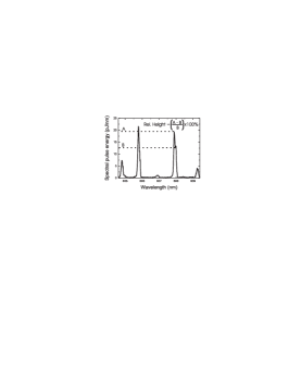
Figure 1: A measured emission spectrum of a gallium phosphide random laser. Our method to determine whether or not a sharp feature is a spike is displayed. We take the spectral pulse energy A at a peak height and the spectral pulse energy B at the highest shoulder of this peak. The formula for the relative height is displayed in the figure. If the relative height is more than 5%, the feature is counted as a spike.

The sample properties and experimental details of our compilation are listed in table 1. The experimental data is presented in table 2 for experiments where spikes occurred in the emission spectrum. When we compare the different experimental data in table 2, we notice that the average Q factor of the laser modes (defined as $\lambda_{e}/w$, with $\lambda_{e}$ in units of energy) is very much alike. Only our own measurement on a porous gallium phosphide random laser (no. 14) has an average Q-factor that is a factor 3 larger. When we compare the heights, we observe that all the height distributions are similar, except for number 9, 10 and 14. The spectra 9 and 10 are from a very special random laser: a photonic crystal with disorder. We conclude that, surprisingly, all experimental results are similar within the uncertainty, except for our own. The reason for this difference could be the very low mean free path $\ell$ of our sample.

	$\ell$		spikes	$w$		$\sigma(w)$		$h$		$\sigma(h)$
	[$\lambda_{e}$]			[cm-1]		[cm-1]		[%]		[%]
Exp.∗	150	.1	13	13	.7 $\pm$	8	.3	27	.3 $\pm$	23	.9
Mod.♮	150	.1	11	13	.9 $\pm$	5	.4	176	$\pm$	380
Exp.∗	920		11	9	.62 $\pm$	3	.49	27	.6 $\pm$	28	.3
Mod.♮	920		6	11	.0 $\pm$	6	.9	199	$\pm$	317

^∗ Exp. = Experiment, ^♮ Mod. = Model.

Table 3: Characterization of the spikes from the experiments and the open-mode model by Mujumdar et al. [3] . The width of the spikes predicted by the model is within one standard deviation of the experimental width. The prediction of the height distribution differs substantially from their experimental result.

Now we will proceed to analyze the models together with the experimental data the apply to. We only found one paper by Mujumdar et al. [3], that showed both the outcome of experiment and a model (the open-mode model). We determined the characteristics of the spikes in both the experimental and theoretical published spectra. The result is listed in table 3. Our comparison between their model and their experiments shows that the width distribution of their experimental spikes extracted by us is predicted correctly by their model. The width is not discussed explicitly in their paper. However, the height distribution extracted by our analysis of their model differs substantially from their experimental result.

In conclusion we have prescribed in this Letter the sets of data needed for a thorough quantitative analysis for both random-laser experiments and models. With these sets a comparison is possible between experiments, and between experiments and models. Surprisingly, all experimental results are similar within the experimental uncertainty except for our own porous gallium phosphide random laser.

This work is part of the research program of the Stichting voor Fundamenteel Onderzoek der Materie (FOM), which is financially supported by the Nederlandse Organisatie voor Wetenschappelijk Onderzoek (NWO). K. van der Molen’s email-address is k.l.vandermolen@utwente.nl.

References

- [1] V. S. Letokhov. Soviet Physics JETP, 26(4):835, 1968.
- [2] N. M. Lawandy, R. M. Balachandran, A. S. L. Gomes, and E. Sauvain. Nature, 368:436, 1994.
- [3] S. Mujumdar, M. Ricci, R. Torre, and D. S. Wiersma. Phys. Rev. Lett., 93(5):053903, 2004.
- [4] D. Anglos, A. Stassinopoulos, R. N. Das, G. Zacharakis, M. Psyllaki, R. Jakubiak, R. A. Vaia, E. P. Giannelis, and S. H. Anastasiadis. J. Opt. Soc. Am. B, 21(1):208, 2004.
- [5] H. Cao, J. Y. Xu, S. H. Chang, and S. T. Ho. Phys. Rev. E, 61(2):1985, 2000.
- [6] X. H. Wu, A. Yamilov, H. Noh, H. Cao, E. W. Seelig, and R. P. H. Chang. J. Opt. Soc. Am. B, 21(1):159, 2004.
- [7] S. V. Frolov, Z. V. Vardeny, A. A. Zakhidov, and R. H. Baughmann. Opt. Comm., 162:241, 1999.
- [8] R. C. Polson and Z. V. Vardeny. Phys. Rev. B, 71:045205, 2005.
- [9] M. A. Noginov, H. J. Caufield, N. E. Noginova, and P. Venkateswarlu. Opt. Comm., 118:430, 1995.
- [10] V. Milner and A. Z. Genack. Phys. Rev. Lett., 94:073901, 2005.
- [11] A. L. Burin, M. A. Ratner, H. Cao, and R. P. H. Chang. Phys. Rev. Lett., 87(21):215503, 2001.
- [12] C. W. J. Beenakker, J. C. J. Paaschens, and P. W. Brouwer. Phys. Rev. Lett., 76:1368, 1996.
- [13] L. Florescu and S. John. Phys. Rev. E, 69:046603, 2004.
- [14] X. Jiang, S. Feng, C. M. Soukoulis, J. Zi, J. D. Joannopoulos, and H. Cao. Phys. Rev. B, 69:104202, 2004.
- [15] M. Patra. Phys. Rev. A, 65:043809, 2002.
- [16] L. I. Deych. Phys. Rev. Lett., 95:043902, 2005.
- [17] L. Angelani, C. Conti, G. Ruocco, and F. Zamponi. Phys. Rev. Lett., 96:065702, 2006.
- [18] A. Yamilov, X. Wu, H. Cao, and A.L. Burin. Opt. Lett., 30:2430, 2005.
- [19] K. L. van der Molen, R. W. Tjerkstra, A. P. Mosk, and A. Lagendijk. arXiv, cond-mat/0612328, 2006.
- [20] K. L. van der Molen, A. P. Mosk, and A. Lagendijk. Phys. Rev. A, 74:053808, 2006.