Influence of symmetry and Coulomb-correlation effects on the optical properties of nitride quantum dots

Abstract

The electronic and optical properties of self-assembled InN/GaN quantum dots (QDs) are investigated by means of a tight-binding model combined with configuration interaction calculations. Tight-binding single particle wave functions are used as a basis for computing Coulomb and dipole matrix elements. Within this framework, we analyze multi-exciton emission spectra for two different sizes of a lens-shaped InN/GaN QD with wurtzite crystal structure. The impact of the symmetry of the involved electron and hole one-particle states on the optical spectra is discussed in detail. Furthermore we show how the characteristic features of the spectra can be interpreted using a simplified Hamiltonian which provides analytical results for the interacting multi-exciton complexes. We predict a vanishing exciton and biexciton ground state emission for small lens-shaped InN/GaN QDs. For larger systems we report a bright ground state emission but with drastically reduced oscillator strengths caused by the quantum confined Stark effect.

I Introduction

The great topical interest in semiconductor nanostructures is not only based on the realization of some of the paradigm of elementary quantum mechanics Michler (2003); Grundmann (2002), but also by the wide range of possible applications, ranging from new Gerard and Gayral (1999); Michler et al. (2000); Santori et al. (2001) and extremely efficient light sources Reithmaier and Forchel (2003) to building blocks for quantum information technology Bouwmeester et al. (2000); Zrenner et al. (2002); Rossi (2004). Further motivation is provided by the possibility to study the effect of reduced dimensions on carrier transport Kouwenhoven et al. (2001) and optical properties Dekel et al. (1998a); Landin et al. (1998); Bayer et al. (2000).

The confinement of the carriers in all three dimensions on a nanometer scale is achieved, for example, by embedding regions of a material with a smaller bandgap in a matrix of a wider bandgap material. A widespread method of creating such quantum dots (QDs) is the Stranski-Krastanow growth mode Nötzel (1996); Jacobi (2003); Stangl et al. (2004).

In this fast evolving research field, nanostructures based on conventional group-III nitrides like AlN, GaN, and InN gained more interest in recent years. Compared to group-III arsenide semiconductor materials, nitride-based nanostructures have the advantage that it is possible to span a much larger spectral range, presently from amber to ultraviolet, by properly alloying together the three building blocks and thereby engineering the direct band gap of these materials Vurgaftman and Meyer (2003).

Nevertheless and despite the intense research on nitride QDs over the last decade the understanding of this material system is – compared to other III-V materials – still in its infancy.

From the theoretical point of view, one challenge is the proper inclusion of effects that stem from the altered atomistic structure of the underlying lattice. While most of the nitrides can crystallize both in the zinc-blende and the wurtzite phase, the latter is by far more stable Morkoc (1999). Additionally, the strong built-in field needs to be considered for, the mostly applied growth along the $c$-axis. In contrast to many other III-V semiconductors, the spin-orbit coupling in the nitrides is rather weak Vurgaftman and Meyer (2003) so that the calculation of the electronic states in terms of a simple effective-mass approximation is not possible due to strong valence band mixing effects. Instead, especially for small nanostructures, a microscopic description of the single-particle states based on, for example, a tight-binding model or pseudo-potential calculation is necessary.

In the past many experimental and theoretical investigations addressed the optical properties of III-V and II-VI QD structures based on, e. g., InGaAs/GaAs or CdSe/ZnSe. One important aspect concerned the analysis of absorption and emission spectra of QDs as a function of the excitation density Barenco and Dupertuis (1995); Hawrylak and Wojs (1996); Dekel et al. (1998a, b); Hawrylak (1999); Bayer et al. (2000); Hohenester and Molinari (2000); Bayer et al. (2002); Bester et al. (2003); Michler (2003). A common result is that the optical processes mainly involve ’diagonal’ transitions, that are connecting, for example, $s$-shell electrons with $s$-shell holes or $p$-shell electrons with $p$-shell holes. In envelope-function approximation this is traced back to dipole matrix elements calculated from the Bloch functions, and interband transition amplitudes determined by the product of dipole matrix elements and the overlap of the electron and hole envelope functions. This picture has been proven to be very fruitful for conventional III-V materials and is oftentimes carried over to the nitride system where emission spectra are then calculated using these ‘diagonal’ excitons. Martin and O’Donnell (1999); Hohenester et al. (1999); DeRinaldis et al. (2002); Shi (2002); Chow and Schneider (2002); DeRinaldis et al. (2004) Our analysis shows, however, that for nitride QDs deviations from this picture are possible. We identify situations, in which the emission is dominated by recombination of ‘skew’ excitons, that are excitons which consist of $s$-shell electrons and $p$-shell holes or vice versa. This led to the prediction of dark exciton and biexction ground state emission. Baer et al. (2005) Such a modified selection rule cannot be explained in an simple effective-mass picture but requires the inclusion of band-mixing effects in a way that properly accounts for the symmetry of the underlying atomic lattice. In addition to the important changes of the optical properties involving one and two excitons, the transitions that occur in systems with a higher population of excitons differ strongly from those known from the InGaAs/GaAs system. While for smaller nitride QDs the “skew” excitons are predicted, we find that in large nitride QDs the energetic order of the $s$-shell and $p$-shell for holes is interchanged, with the $p$-shell being lowest in energy. This leads to optically active exciton transitions. Schulz et al. (2006) However, as a result of the quantum confined Stark effect (QCSE), with increasing height of the QDs the corresponding dipole matrix elements decrease drastically Andreev and O’Reilly (2001); DeRinaldis et al. (2002); Schulz et al. (2006) due to the separation of the electron and hole wave functions in the strong internal electric field. In combination with the dark exciton state in small nitride QDs, this makes the application of nitride QDs more challenging.

In this work we study the multi-exciton emission spectra in nitride QDs and discuss the resulting complicated peak structure in detail. Restricting ourselves to the two lowest shells allows even a semi-analytic description of the problem. The single-particle states are deduced from an atomistic tight-binding model as briefly outlined in Sec. II. Even without a detailed calculation of the single-particle states, the symmetry considerations of Sec. III can be used to draw conclusions regarding the dipole-matrix elements and the multi-exciton spectra. In Sec. IV the Hamiltonian of the interacting charge carrier system and the configuration interaction (CI) scheme are presented. Results for an initial filling with up to six excitons are provided in Section V.2 and major trends are discussed in Section V.3 in terms of an approximate Hamiltonian. Further details of the multi-exciton spectra are analyzed in Section VI In the subsequent Section VII the influence of the strong built-in field is investigated. Finally, the spectra for a larger nitride QD are presented in Section VIII and compared to those found for the smaller structure.

II Electronic structure

For a proper treatment of the single particle states in nitride systems, an atomistic multiband approach, like pseudopotential or tight-binding (TB) models, is required. General aspects for the developement of such a TB approach and the calculation of dipole and Coulomb matrix elements are discussed in detail in Ref. Schulz et al., 2006. In the following Section II.1, we briefly summarize the main ingredients of the subsequently used TB model, while Sections II.2 and  II.3 are devoted to details of the calculation of single-particle states and interaction matrix elements.

II.1 Tight-Binding model and built-in field

For the calculation of the single-particle states we use a TB model with an $sp^{3}$ basis $|\alpha\rangle_{\mathbf{R}}$, that contains one $s$-state ($\alpha=s$) and three $p$-states ($\alpha=p_{x},p_{y},p_{z}$) per spin direction at each atomic site $\mathbf{R}$. The $i^{\mathrm{th}}$ TB single-particle wave function is given by

$$|\phi_{i}\rangle=\sum_{\alpha,\mathbf{R}}|\alpha\rangle_{\mathbf{R}}\,c^{i}_{\alpha}(\mathbf{R})$$

with the expansion coefficients denoted by $c^{i}_{\alpha}(\mathbf{R})$. We assume a lens-shaped InN QD, grown in (0001)-direction on top of an InN wetting layer (WL), that is embedded in a GaN matrix. For the numerical evaluation, a finite wurtzite lattice within a supercell with fixed boundary conditions is chosen. The small spin-orbit coupling and crystal-field splitting are neglected Vurgaftman and Meyer (2003). Furthermore, we neglect the strain induced displacement of the atoms. For the used QD geometry, a more realistic inclusion of strain effects does not change the symmetry of the system and henceforth the general statements discussed in this paper should not be affected. In the following we consider two different QD sizes with diameters $d=4.5,5.7$ nm and heights $h=1.6,2.3$ nm, respectively. In both cases a WL thickness of one lattice constant $c$ is assumed.

In contrast to cubic III-V semiconductor heterostructures, e.g., InAs or GaAs, the III-V wurtzite nitrides exhibit considerable larger built-in fields Bernardini et al. (1997), which can significantly modify both the electronic and the optical properties. This field enters via the electrostatic potential as a site-diagonal contribution $V_{p}(\mathbf{R})=-e\phi_{p}(\mathbf{R})$ to the TB Hamiltonian. Sala et al. (1999); Saito and Arakawa (2002)

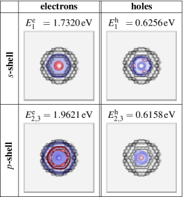
Figure 1: (color online). Top view of the QD structrue with the first two bound shells for electrons (left) and holes (right). Depicted are isosurfaces of the probability density with 20% (blue) and 80% (red) of the maximum value are shown. Only one state is visualized for the two-fold degenerate $p$-shell, as the other looks alike. The corresponding energies ($E^{e,h}_{1,2,3}$) are measured relative to the valence band maximum of the bulk GaN.

II.2 Single-particle states

The small QD ($d=4.5$ nm, $h=1.6$ nm) confines three bound states for the electrons. The corresponding probability densities of the first two bound shells for electrons and holes are presented in Fig. 1. In the calculation, the influence of the built-in field was included. The dominant contribution for the electron single-particle states stems from the atomic $s$-orbitals, while for the hole states a strong intermixing of the atomic $p$-orbitals is observed. This is indicative for the fact that a suitable description of the one-particle states and the resulting optical properties requires a multi-band approach and cannot be accounted for in a one-band effective mass approximation.

If one compares the single-particle states with and without the inclusion of the built-in field, Schulz et al. (2006) one finds that, in the presence of the field, the electron states are squeezed into the cap of the QD while the hole states are constraint to a few atomic layers at the bottom near the WL. This effect is even more pronounced for the larger QD ($d=5.7$ nm, $h=2.3$ nm). In this case a clear spatial separation of electron and hole wave functions is observed, which lowers the direct spatial overlap between the two and leads to strongly reduced dipole matrix elements. Furthermore, as known from the QCSE, the built-in field leads to an overall red-shift in the single-particle transition energies. In addition, we find for the large QD, that the ordering of the energy levels is affected by the built-in field. Specifically we obtain that in the presence of the built-in field the level ordering for the holes is reversed so that the ground state is formed by the two-fold degenerate states $\phi^{h}_{2,3}$ ($p$-shell in Fig. 1) while the first excited state $\phi^{h}_{1}$ (s-shell in Fig. 1) is nondegenerate. This is in contrast to the observed level ordering of the large QD in the absence of the built-in field or of the small QD with and without the field. In these cases, the ground state is nondegenerate ($\phi^{h}_{1}$) and the first two excited states are degenerate ($\phi^{h}_{2,3}$). Such a behavior has been reported before for other QD systems and a detailed discussion can be found in Ref. Schulz et al., 2006.

II.3 Evaluation of dipole- and interaction matrix elements

Based on the TB single-particle wave-functions one can determine dipole- and Coulomb matrix elements that are crucial for the calculation of optical properties. As emphasized above, a TB model represents an atomistic approach to describe the electronic structure of low-dimensional heterostructures. Explicit knowledge about a basis set of localized (Wannier) states is not required for the calculation of one-particle energies and wave functions, because the Hamiltonian matrix elements between the different orbitals are treated as parameters within the TB model. What enters the TB calculation are only the basic assumptions about the localized (atomic) orbitals: symmetry, spatial orientation Slater and Koster (1954), and orthogonality.

For the calculation of interaction matrix elements one needs – at least in principle – the localized basis states. For the Coulomb matrix elements, however, the explicit knowledge of the atomic orbitals is not required in practice, as these matrix elements are dominated by long-range contributions in which the local orbitals act as point charges. The structure of the localized orbitals is of significance only for on-site and nearest-neighbor interactions, which in our calculation contribute less than $5\,\%$ to the total Coulomb matrix elements. These findings are in agreement with Ref. Sun and Chang, 2000. Thus, the matrix elements are approximated by a sum over the TB coefficients $c_{\alpha}^{i}(\mathbf{R})$ at atom sites $\mathbf{R},\mathbf{R}^{\prime}$ with orbital indices $\alpha,\beta$:

$$V_{ij,kl} =\int d^{3}r\int d^{3}r^{\prime}\;\phi_{i}^{*}(\mathbf{r})\phi_{j}^{*}(\mathbf{r}^{\,\prime})V(\mathbf{r}-\mathbf{r}^{\,\prime})\phi_{k}(\mathbf{r}^{\,\prime})\phi_{l}(\mathbf{r})$$

$$\approx\sum_{\mathbf{R}\mathbf{R}^{\prime}}\sum_{\alpha\beta}c_{\alpha}^{i\ast}(\mathbf{R})c_{\beta}^{j\ast}(\mathbf{R}^{\prime})c^{k}_{\beta}(\mathbf{R}^{\prime})c^{l}_{\alpha}(\mathbf{R})\,V(\mathbf{R}-\mathbf{R}^{\prime})$$

with $$\quad V(\mathbf{R}-\mathbf{R}^{\prime})=\frac{e^{2}}{4\pi\varepsilon_{0}\varepsilon_{r}|\mathbf{R}-\mathbf{R}^{\prime}|}\quad\text{for}\quad\mathbf{R}\not=\mathbf{R}^{\prime}$$

and $$\quad V(0)=\frac{1}{v^{2}_{uc}}\int_{uc}d^{3}r\,d^{3}r^{\prime}\frac{e^{2}}{4\pi\varepsilon_{0}\varepsilon_{r}|\mathbf{r}-\mathbf{r}^{\prime}|}\;.$$

The labels $i,j,k,l$ refer either to electron or to hole states in order to consider the repulsive electron-electron and hole-hole interaction, as well as the attractive electron-hole interaction. The considerably smaller matrix elements of the electron-hole exchange interaction are neglected. The calculation of the onsite integrals $V(0)$ involves the integration over the volume of the unit cell $v_{uc}$ and can be done quasi-analytically by expansion of the Coulomb interaction in terms of spherical harmonics. Schnell et al. (2002) The electronic charge and the vacuum dielectric constant are denoted by $e$ and $\epsilon_{0}$, respectively. We use the InN dielectric constant $\varepsilon_{r}=8.4$ according to Ref. Shi and Gan, 2003 since the wave functions are almost completely confined inside the QD.

For the calculation of dipole matrix elements $\mathbf{d}^{eh}_{ij}\propto\langle\phi^{e}_{i}|\mathbf{r}|\phi^{h}_{j}\rangle$, the explicit structure of the localized orbitals is needed as the dipole-operator is dominated by short-range contributions. Though being not orthogonal at different sites, standard Slater orbitals Slater (1930) have been used in earlier calculations Lee et al. (2001, 2002) within orthogonal TB models. While they include the correct symmetry properties, the missing orthogonality limits their applicability. To overcome this problem, we use numerically orthogonalized Slater orbitals Schulz et al. (2006) and account for the slight non-locality of the dipole operator Leung et al. (1998) and the underlying anion-cation structure of the crystal by including also contributions from up to second-nearest neighbors.

III Symmetry considerations

The specific symmetry of the system under consideration plays an important role in the prediction of energy degeneracies and optical selection rules. The overall symmetry of the problem is determined by two factors: (i) the crystal symmetry of the underlying lattice and (ii) the symmetry of the QD geometry or, more generally, the geometry of the heterostructure.Bester and Zunger (2005)

The interplay between the dot geometry and the underlying lattice is well illustrated by the example of the lens-shaped QD. The geometry of the QD has a $C_{\infty v}$ symmetry.Wilson et al. (1955) In the effective mass approximation or in the $\mathbf{k}\cdot\mathbf{p}$ theory the underlying atomic structure is not resolved, so that one obtains degenerate energies for the lens-shaped QD. Wojs et al. (1996); Jacak et al. (1998); Bester and Zunger (2005) However, if one takes the crystal structure into account, as it is done, in a TBSchulz and Czycholl (2005); Schulz et al. (2006) or pseudo-potential calculation Bester and Zunger (2003), the symmetry will be reduced and degeneracies can be lifted.Bester and Zunger (2005) For a lens-shaped QD grown on a wurtzite lattice along the (0001)-direction, the symmetry is reduced to $C_{3v}$. If a QD with the same geometry is grown in the zinc-blende phase in (001)-direction, one is left with an even lower $C_{2v}$ symmetry. As we will discuss in the next subsection, the former group is still rich enough to predict degeneracies, while the latter is too small to support degenerate eigenstates.

III.1 Energy spectrum

The $C_{3v}$ group is generated by the rotation around the $z$-axis with an angle of $2\pi/3$, denoted by $C_{3z}$, together with a mirror reflection at a plane perpendicular to the $y$-axis, denoted by $IC_{2y}$. Cornwell (1969) These operations commute with the Hamiltonian, but not among themselves. From this non-abelian character of the group one can immediately conclude that there must exist energetically degenerate states. In the case of the wurtzite QD under consideration, one example of such degenerate states are the $p$-shell levels given in Fig. 1.

This degeneracy in the wurtzite structure is especially worth mentioning in view of a recent paper Bester and Zunger (2005) in which it is argued that a description at the atomic level in zinc-blende-based QDs should remove the $p$-shell degeneracy. The argument is essentially the following: the four-fold rotation is part of the zinc-blende point group only if followed by the inversion, but many high symmetry (lens-shaped, pyramidal) QDs forbid the inversion and with it the $C_{4v}$ symmetry. One is therefore left with a $C_{2v}$ point group, which is abelian and therefore insufficient for $p$-degeneracy.

This conclusion is correct, but it cannot be carried over to the wurtzite QDs, because in wurtzite crystals the three-fold rotation holds without inversion. If the QD geometry is sufficiently symmetric (lens-shaped, hexagonal pyramids) then the problem retains the $C_{3v}$ symmetry, which leads to $p$-degeneracy. In papers predicting $p$-shell splitting for QDs in wurtzite lattices and neglecting the spin-orbit coupling Andreev and O’Reilly (2000); Fonoberov and Balandin (2003), either boundary conditions or discretization meshes spoil the correct $C_{3v}$ symmetry of the problem. Therefore the small $p$-shell splitting obtained there is a numerical artefact. On the contrary the splitting induced by the inclusion of the spin-orbit coupling Winkelnkemper et al. (2006), albeit quite small, is physically correct.

To summarize the discussion, for a lens-shaped QD and in the absence of the spin-orbit coupling a degeneracy of the $p$-shell is expected in the wurtzite phase but not in a zinc-blende structure.

III.2 Single-particle states

So far we discussed only the role of symmetry on the energy spectrum. Turning now to the dipole selection rules, one should consider the symmetry properties of the wave functions. In the TB description the wave functions are expanded in the atomic orbital basis according to

$$|\phi\rangle=\sum_{\mathbf{R}}|s\rangle_{\mathbf{R}}\;a(\mathbf{R})+\sum_{\mathbf{R},j}|{p_{j}}\rangle_{\mathbf{R}}\;b_{j}(\mathbf{R})\,\,,$$ (1)

where $|s\rangle_{\mathbf{R}}$ denotes the atomic $s$-orbital centered around the site $\mathbf{R}\>$ with $\langle\mathbf{r}|s\rangle_{\mathbf{R}}=\psi_{s}(\mathbf{r}-\mathbf{R})$, and the corresponding $p$-orbitals follow similarly from $|p_{j}\rangle_{\mathbf{R}}$ with $j=x,y,z$. The expansion coefficients are given by $a(\mathbf{R})$ and $b_{j}(\mathbf{R})$, respectively.

The action of a symmetry operation $T$ on the wave function is defined via Inui et al. (1990); Cornwell (1969)

$$(T\phi)(\mathbf{r})=\phi(T^{-1}\mathbf{r}).$$ (2)

In the case of the TB wave function, Eq. (1), this amounts to a simultaneous transformation of the orbitals and of their centers. Instead of the original orbitals $p_{x}$ and $p_{y}$, it is more convenient to work with the complex combinations $p_{\pm}=(p_{x}\pm ip_{y})/\sqrt{2}$ which are angular-momentum eigenstates.

For a wurtzite QD with $C_{3v}$ symmetry one has to consider the transformation properties of the orbitals under the discrete $2\pi/3$ rotation $C_{3z}$ around the $z$-axis and the mirror reflection $IC_{2y}$, defined by $(x,y,z)\rightarrow(x,-y,z)$. While the atomic $s$ and $p_{z}$ orbitals do not change under these transformations, the remaining $p_{\pm}$ orbitals transform like

$$C_{3z}|p_{+}\rangle =e^{-i\frac{2\pi}{3}}|p_{+}\rangle\;,\quad IC_{2y}|p_{+}\rangle =|p_{-}\rangle\;,$$ (3)

$$C_{3z}|p_{-}\rangle =e^{+i\frac{2\pi}{3}}|p_{-}\rangle\;,\quad IC_{2y}|p_{-}\rangle =|p_{+}\rangle.$$

Using Eq. (2) these transformation properties of the local orbitals under the group basic rotations are carried over to the total wave function, given by Eq. (1). This defines the action of the group on the TB basis and allows the classification of the eigenstates according to the irreducible representations of the $C_{3v}$ group. States which are invariant under the action of the group will be called $s$-states and will be denoted by $|\phi_{s}\rangle$. This terminology and notation are somewhat lax since according to it a $p_{z}$-orbital is also an $s$-state. Nevertheless we use them for the sake of simplicity and in agreement with the literature. Similarly, the basis vectors of a two-dimensional representation changing under the group operations like in Eq. (3) will be called $p_{\pm}$-states and will be denoted $|\phi_{p_{\pm}}\rangle$.

As an example, it can be shown that an $s$-state wave function must have the form

$$|\phi_{s}\rangle = \sum_{\mathbf{R}}\big{[}\;|s\rangle_{\mathbf{R}}\;\alpha(\mathbf{R})+|p_{z}\rangle_{\mathbf{R}}\;\beta_{z}(\mathbf{R})\;\big{]}$$

$$+\sum_{\mathbf{R}}\big{[}\;|p_{+}\rangle_{\mathbf{R}}\;\mathcal{Z}^{*}_{\mathbf{R}}\;\beta(\mathbf{R})+|p_{-}\rangle_{\mathbf{R}}\;\mathcal{Z}_{\mathbf{R}}\;\beta^{*}(\mathbf{R})\big{]}$$

where the coefficients $\alpha(\mathbf{R})$, $\beta_{z}(\mathbf{R})$, and the real part of $\beta(\mathbf{R})$ are invariant under all rotations of $C_{3v}$, while the imaginary part of $\beta(\mathbf{R})$ is invariant under the proper rotation $C_{3z}$ but changes sign under the action of the improper rotation $IC_{2y}$. The quantity $\mathcal{Z}_{\mathbf{R}}$ is defined as ${X}_{\mathbf{R}}+i{Y}_{\mathbf{R}}$ or in polar coordinates $\sqrt{X_{\mathbf{R}}^{2}+Y_{\mathbf{R}}^{2}}e^{i\xi_{\mathbf{R}}}$, where ${X}_{\mathbf{R}}$ and ${Y}_{\mathbf{R}}$ denote the in-plane cartesian coordinates of the lattice site $\mathbf{R}$ and $\xi_{\mathbf{R}}$ is the polar angle of the point $\mathbf{R}$ in cylindrical coordinates. It is clear that with $\alpha(\mathbf{R})$, $\beta_{z}(\mathbf{R})$ rotation invariant the first sum in Eq. (III.2) is $s$-like. In the second sum one has a compensation between the $p$-behavior of the orbitals and that of the $\mathcal{Z}_{\mathbf{R}}$ coefficients leading to a combination which is left invariant by the rotations. The equivalent of this situation in a $\mathbf{k}\cdot\mathbf{p}$ approach would be expressed by the $p$-character of the envelopes multiplying to the $p_{\pm}$-type Bloch functions and compensating the phase factor acquired under rotation in order to produce full invariance. In this way, the coefficients of the expansion Eq. (III.2) can be seen as discretized versions of the envelope function components.

For the electron and hole wave functions whose modulus square is depicted in Fig. 1 the lowest-lying levels are indeed invariant under the action of the elements of the discrete group and therefore represent $s$-states. As expected, the electron $s$-state consists mainly of $s$ atomic orbitals, i. e. the dominant coefficient is $\alpha(\mathbf{R})$, which is $C_{3v}$-invariant as stated above. This state looks very similar to what would be expected for an $s$-state in the effective mass approximation: it is symmetric under rotation, has a single maximum at the center and decays to the boundaries. In contrast, the shape of the ground state of the holes does not show the same behavior. It shows the (discrete) rotational symmetry, but has a node at the center. This state is expected to consist mainly of $p$ atomic orbitals and indeed, an inspection of its coefficients shows that the second sum in Eq. (III.2) is dominant. Since  Fig. 1 displays the sum of the modulus square of the expansion coefficients, one obtains $2|\mathcal{Z}^{*}_{\mathbf{R}}\;\beta(\mathbf{R})|^{2}=2(X_{\mathbf{R}}^{2}+Y_{\mathbf{R}}^{2})|\beta(\mathbf{R})|^{2}$, which explains both the rotational symmetry and the vanishing value at the origin. In other words the unexpected node at the origin stems from the $p$-character of the coefficients.

A similar analysis of the coefficients can be carried out for the excited states ($p$-shell), and reveals that these states have indeed the $|\phi_{p_{\pm}}\rangle$ symmetry.

III.3 Dipole-matrix elements

The numerical evaluation of the dipole-matrix elements shows that the non-zero values of the in-plane dipole matrix elements $\mathbf{e}\mathbf{d}^{eh}_{ij}$ with $\mathbf{e}$ in the $x$-$y$-plane are much larger than those with $\mathbf{e}$ in $z$-direction. Therefore we consider here only the in-plane matrix elements with $\mathbf{e}=1/\sqrt{2}(1,1,0)$ and denote the corresponding dipole-matrix elements by $d^{eh}_{ij}$. Furthermore the matrix elements ${d}^{eh}_{p_{i}p_{j}}$, with $i,j\in\{x,y\}$ are more than one order of magnitude smaller than the other non-vanishing matrix elements. As a consequence, these contribution can safely be neglected in the calculation of optical spectra, in which the absolute value of the dipole-matrix elements enters even quadratically. As explained below, it turns out that these results can be understood on symmetry grounds.

To this end we consider the matrix elements $\langle\l_{z}|x\pm iy|\l^{\prime}_{z}\rangle$, from which all the in-plane dipole matrix elements can be deduced by linear combinations and are characterized by simple transformation properties. Here we denote the states $|l_{z}\rangle$ by the phase factor $e^{-i\l_{z}\theta}$ they pick up under a rotation around the $z$-axis of the angle $\theta$, that is, $\l_{z}=0$ for the $s$-state and $\l_{z}=\pm 1$ for the $p_{\pm}$-states. Using the transformation properties of the wave functions and those of $x\pm iy$ under rotation, one can rewrite the matrix elements as

$$\langle\l_{z}|x\pm iy|\l^{\prime}_{z}\rangle=e^{i(\l_{z}-\l_{z}^{\prime}\mp 1)\theta}\langle\l_{z}|x\pm iy|\l_{z}^{\prime}\rangle{.}$$ (5)

In a $C_{\infty v}$ group the angle $\theta$ is arbitrary and one would obtain the familiar result that the dipole matrix elements $d^{eh}_{\l_{z},\l_{z}^{\prime}}$ can only be non-zero for $\l_{z}-\l_{z}^{\prime}=\pm 1$. In particular one has $d^{eh}_{ss}=0=d^{eh}_{p_{i},p_{j}}$ with $i,j\in\{\pm 1\}$ and only $d^{eh}_{s,p_{i}}$ and $d^{eh}_{p_{i},s}$ can be non-zero.

In case of the $C_{3v}$ symmetry the allowed values for the angle $\theta$ are only the integer multiples of $2\pi/3$. Then one finds the weaker result that the condition for non-zero dipole matrix elements is $\l_{z}-\l_{z}^{\prime}=\pm 1\text{ modulo }3$. This means that the discussed symmetry reduction opens additional decay channels. One still has $d^{eh}_{ss}=d^{eh}_{p_{+}p_{+}}=d^{eh}_{p_{-}p_{-}}=0$ but, in addition to $d^{eh}_{p_{\pm},s}$, $d^{eh}_{s,p_{\pm}}$, now also the matrix elements $d^{eh}_{p_{+}p_{-}}$ and $d^{eh}_{p_{-}p_{+}}$ can be non-zero. Nevertheless, since the last two are vanishing in case of a continuous rotation symmetry, it is quite plausible that they remain small even in the case of a three-fold axis. This behavior is found by the numerical evaluation of the dipole matrix elements. In our example of the small QD we find $|d^{eh}_{p_{+}p_{-}}|^{2}=4.84\times 10^{-4}$ $(\text{\AA})^{2}$, which is negligible in comparison with $|d^{eh}_{sp_{\pm}}|^{2}=4.73$ $(\text{\AA})^{2}$.

As we will see in Section V these selection rules, and in particular the vanishing dipole matrix element $d^{eh}_{ss}$, have very important consequences for the optical properties of nitride QDs.

III.4 Coulomb matrix elements

Table 1: All nonzero electron-electron Coulomb matrix elements determined numerically from the TB-wave functions. The index 0 denotes the $s$-state $|\phi_{s}\rangle$ and $\pm$ denote the states $|\phi_{p_{\pm}}\rangle$. The matrix elements below the horizontal double line would be zero in the case of a $C_{\infty v}$ symmetry. Explicit values are given for of the small the small QD but without the inclusion of the internal electrostatic field.

(i,j,k,l)	$V^{ee}_{ijkl}$ [meV]
(0,0,0,0)	93.8459
(0,+,+,0) , (0,-,-,0) , (+,0,0,+) , (-,0,0,-)	81.6389
(-,-,-,-) , (+,+,+,+) , (+,-,-,+) , (-,+,+,-)	75.8542
(0,0,+,-) , (0,0,-,+) , (+,-,0,0) , (-,+,0,0)	17.0949
(0,+,0,+) , (+,0,+,0) , (0,-,0,-) , (-,0,-,0)	17.0949
(+,-,+,-) , (-,+,-,+)	9.3997
(+,0,-,-) , (+,+,0,-) , (-,0,+,+) , (-,-,0,+)	-0.1972
(0,+,-,-) , (+,+,-,0) , (0,-,+,+) , (-,-,+,0)	-0.1972

It is possible to use the same kind of symmetry arguments for the calculation of the Coulomb matrix elements. Again we find that a three-fold symmetry axis allows for more non-zero elements than a $C_{\infty z}$-axis. Nevertheless, these additional matrix elements are rather small. If the entire system is rotated by an angle $\theta=\frac{2\pi}{3}$, each single-particle wave function acquires a phase factor, while the distance $|\mathbf{r}-\mathbf{r}^{\prime}|$ is not affected by this rotation. Therefore we find for the interaction matrix elements:

$$V_{ijkl}=e^{i(\lambda^{z}_{i}+\lambda^{z}_{j}-\lambda^{z}_{k}-\lambda^{z}_{l})\theta}V_{ijkl}\quad.$$ (6)

From this one can deduce that $V_{ijkl}$ must be zero if $\lambda^{z}_{i}+\lambda^{z}_{j}-\lambda^{z}_{k}-\lambda^{z}_{l}\neq 0\;\text{modulo}\;3$. The $z$-projection of the angular momentum is conserved only modulo 3, and not exactly, as it would be in the case for a continuous rotation axis $C_{\infty z}$. Baer et al. (2004). This gives rises to additional non-zero matrix elements $V_{ijkl}$. Examples for the electron-electron $V_{ijkl}$ are given in Tab. 1 using here the ($s$,$p_{+}$,$p_{-}$) representation. Clearly these additional matrix elements are rather small. This is in accordance with our expectation about matrix elements that would altogether vanish in a system with a higher symmetry.

Symmetry is also responsible for some Coulomb matrix elements having equal values. Such cases are grouped in Tab. 1 between horizontal lines.

IV Many Body Problem

IV.1 Hamiltonian

So far we discussed only the single-particle properties. However, the investigation of optical properties is an inherent many-particle problem. The Hamiltonian $H$ that describes the system of interacting electrons and holes in a QD consists of two parts:

$$H_{0}= \sum_{i\sigma}\varepsilon^{e}_{i}e^{{\dagger}}_{i\sigma}e_{i\sigma}+\sum_{i\sigma}\varepsilon^{h}_{i}h^{{\dagger}}_{i\sigma}h_{i\sigma}\quad,$$

$$H_{\text{Coul}}= \frac{1}{2}\sum_{ijkl\atop\sigma\sigma^{\prime}}V^{ee}_{ij,kl}\;e^{{\dagger}}_{i\sigma}e^{{\dagger}}_{j\sigma^{\prime}}e_{k\sigma^{\prime}}e_{l\sigma}$$

$$+\frac{1}{2}\sum_{ijkl\atop\sigma\sigma^{\prime}}V^{hh}_{ij,kl}\;h^{{\dagger}}_{i\sigma}h^{{\dagger}}_{j\sigma^{\prime}}h_{k\sigma^{\prime}}h_{l\sigma}$$

$$-\sum_{ijkl\atop\sigma\sigma^{\prime}}V^{he}_{ij,kl}\;h^{{\dagger}}_{i\sigma}e^{{\dagger}}_{j\sigma^{\prime}}e_{k\sigma^{\prime}}h_{l\sigma}\quad.$$ (7)

The free part $H_{0}$ contains information about the single-particle spectrum $\varepsilon_{i}^{(e,h)}$ and describes a system of non-interacting charge carriers. Here $e_{i\sigma}$ ($e^{{\dagger}}_{i\sigma}$) are annihilation (creation) operators of electrons with spin $\sigma$ in the one-particle states $|i\rangle$ of energy $\varepsilon^{e}_{i}$. The corresponding operators and single-particle energies for holes are $h_{i\sigma}$ ($h^{{\dagger}}_{i\sigma}$) and $\varepsilon^{h}_{i}$, respectively. The electron-electron, hole-hole and electron-hole Coulomb interaction between the charged carriers is included in $H_{\text{Coul}}$. The Coulomb matrix elements $V_{ij,kl}$ are determined from the TB single particle wave functions, as described in Sec. II.3.

IV.2 Configuration interaction (CI)

In a semiconductor QD the finite height of the confinement potential leads to a finite number of localized states as well as to a continuum of energetically higher delocalized states. If one considers only the energetically lowest single-particle states, the eigenvalue problem for a given number of electrons and holes has a finite (albeit large) dimension and can be solved without further approximations.

As the Hamiltonian $H$ conserves the total number of electrons $N_{e}$ and holes $N_{h}$, the Hamiltonian matrix falls into subblocks with basis states corresponding to uncorrelated many-particle states of the form

$$|\phi\rangle=\prod_{\begin{subarray}{c}i\end{subarray}}(e^{{\dagger}}_{i})^{n^{e}_{i}}\prod_{\begin{subarray}{c}j\end{subarray}}(h^{{\dagger}}_{j})^{n^{h}_{j}}\,\,|0\rangle\quad,$$ (8)

with the occupancy numbers $n^{e,h}_{i}=0,1$ and $\sum_{i}n_{i}^{e}=N_{e}$, $\sum_{j}n_{j}^{h}=N_{h}$. In order to find the eigenvalues and eigenfunctions of the interacting problem, the Hamiltonian $H$, Eq. (IV.1), is expressed in terms of the uncorrelated basis states $|\phi\rangle$, Eq. (8). The resulting Hamiltonian matrix is then diagonalized numerically. In this way one finds an expansion of the interacting eigenstates for a given number of electrons and holes in terms of the uncorrelated basis states of the system. These states can be used to calculate, for example, the interband emission spectra between the interacting Coulomb correlated eigenstates of the QD system using Fermi’s golden rule:

$$I(\omega)={2\pi\over\hbar}\sum_{f}|\langle\phi_{f}|H_{\text{d}}|\phi_{i}\rangle|^{2}\,\,\delta(E_{i}-E_{f}-\hbar\omega)\quad.$$ (9)

Here $|\phi_{i}\rangle$ denotes the correlated initial state with energy $E_{i}$ and $|\phi_{f}\rangle$ and $E_{f}$ the corresponding quantities of the final states. A similar equation holds for the absorption spectrum. The Hamiltonian $H_{\text{d}}$ describes the light matter interaction in dipole approximation

$$H_{\text{d}}=-e|\mathbf{E}|\sum_{n,m}\langle n|\mathbf{r}\mathbf{e}_{p}|m\rangle h^{{\dagger}}_{n,\sigma}e^{{\dagger}}_{m,-\sigma}+\text{h.c.}{,}$$ (10)

with $\mathbf{E}$ being the electric field at the position of the QD, $\mathbf{e}_{p}$ is the polarization vector, and $e$ is the elementary charge. Furthermore the states $|n\rangle$ and $|m\rangle$ denote hole and electron single-particle states, respectively. Fermi’s golden rule, Eq. (9), implies that the optical field always creates or destroys electron-hole pairs. Hence the initial and final states differ by exactly one electron-hole pair. For the following discussion it is convenient to express the dipole Hamiltonian in terms of the interband polarization operator $\mathcal{P}$ according to $H_{\text{d}}=-e|\mathbf{E}|(\mathcal{P}+\mathcal{P}^{\dagger})$.

If the analysis is restricted to $s$- and $p$-shells and the small dipole matrix elements $d^{eh}_{p_{-}p_{+}}$ and $d^{eh}_{p_{+}p_{-}}$ are neglected, one can split $\mathcal{P}$ into $\mathcal{P}_{\text{low}}$ and $\mathcal{P}_{\text{high}}$ according to:

$$\mathcal{P}_{\text{high}} =\sum_{\sigma}\Big{(}d^{eh}_{ps}\;e_{p_{+},\sigma}h_{s,-\sigma}+d^{eh*}_{ps}\;e_{p_{-},\sigma}h_{s,-\sigma}\Big{)}\,,$$ (11)

$$\mathcal{P}_{\text{low}} =\sum_{\sigma}\Big{(}d^{eh}_{sp}\;e_{s,\sigma}h_{p_{+},-\sigma}+d^{eh*}_{sp}\;e_{s,\sigma}h_{p_{-},-\sigma}\Big{)}\,.\;\;$$

This is motivated by the fact that the single-particle energy separation for the electrons is larger than for the holes.

V Optical Properties

To be able to distinguish between effects stemming from the symmetry group of the QD and those additionally introduced by the internal electric field, we will first present the results where the built-in field is artificially switched off. In a second step, we will discuss the influence of this field on the multi-exciton spectra.

V.1 Excitonic and biexcitonic properties

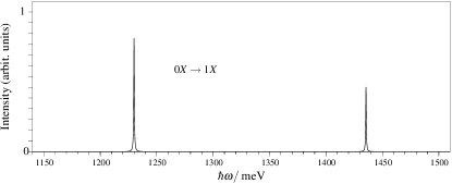
Figure 2: Absorption spectrum of the initially empty nitride QD. The high-energy side stems from a transition in which mainly the $s$-shell of the hole and the $p$-shell for the electrons is occupied. For the low-energy side the $s$-shell of the electrons and the $p$-shell of the holes yield the main contribution.

The considered small QD confines only three bound electron states ($s$- and $p$-shell) for each spin polarization. These states enter the CI approach, together with the hole $s$- and $p$-shells, which are energetically well separated from the other localized states. The corresponding excitonic absorption spectrum shows the two lines depicted in Fig. 2. Here we denote an electron-hole pair, in which the electron has mainly $\alpha$ and the hole mainly $\beta$ character, as an $\alpha\beta$-exciton with $\alpha,\beta\in\{s,p\}$. We found in Section III.3 that in the nitride case the transitions do not originate from ’diagonal’ $ss$- and $pp$-excitons, as one may expect, but from $sp$- and $ps$-excitons. Because of the large energy splitting between the $s$- and the $p$-shell of the electrons, the $ps$-excitonic transition is well separated from the $sp$ transition. Without Coulomb interaction, these transitions can be found at the sum of the single-particle energies $\epsilon_{p}^{e}+\epsilon_{s}^{h}$ and $\epsilon_{s}^{e}+\epsilon_{p}^{h}$, respectively. For the absorption spectrum the unusual selection rules described in Sec. III.3 and the resulting “skew” excitons lead only to quantitative changes. Even if the optical spectra could be described in terms of diagonal excitons, one would still obtain two lines in the absorption spectrum Hawrylak (1999), one from the $s$-shell and one involving the $p$-shell carriers. However, for the emission spectrum the changes are quite important. Most importantily the exciton and biexciton ground state for small InN/GaN QDs remain dark. Baer et al. (2005) This is the case because the excitonic and biexcitonic ground states are dominated by those configurations where all the carriers are in their energetically lowest shell together with the fact that the dipole-matrix element $d^{eh}_{ss}$ involving these states vanishes.

V.2 CI results for multi-exciton emission spectra

Only for more than two excitons the CI calculation provides significant population of the electron and hole $p$-shells. Then emission processes involving the ‘skew’  excitons can take place. As mentioned above the low- and high-energy side of the spectrum can be attributed to processes where an $s$-electron or a $p$-electron is dominantly involved in the recombination process, respectively. A schematic representation of the level-structure and electron-hole pairs typically involved in high- and low-energy transitions is depicted in Fig. 3.

An inspection of the emission-spectra reveals a blue-shift as the number of excitons is increased. This is in strong contrast to the results known from the InGaAs system Bayer et al. (2000); Dekel et al. (2000); Baer et al. (2004) but can be explained in terms of the diagonal Hamiltonian, discussed in the next section, and the fact that the envelopes for the electrons and holes differ strongly. Also it can be seen that, with the exception of the $5X\rightarrow 4X$ transition, all spectra are rather similar if one compares the line structure of the low- and high-energy side. On the other hand, the oscillator strengths of the peaks on the high-energy side are systematically weaker than the corresponding ones at the low-energy side. These aspects will be addressed in the following in detail.

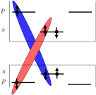
Figure 3: (color online) For the example of a three exciton state, the light (red) and dark (blue) shaded areas connect the carriers that will lead to an emission at the low- and high-energy side of the spectrum, respectively.

V.3 Diagonal approximation

As discussed in Ref. Baer et al., 2004, an approximate description using a Hamiltonian that is diagonal in the free states can be motivated by inspecting the relative importance of the various Coulomb matrix element. The eigenvalues of this approximate Hamiltonian are then the non-selfconsistent Hartree-Fock energies. This approximation has successfully been used to describe the dominant trends in multi-exciton spectra in III-V systems. Dekel et al. (2000); Franceschetti et al. (2000); Shumway et al. (2001); Bester and Zunger (2003); Ulrich et al. (2005)

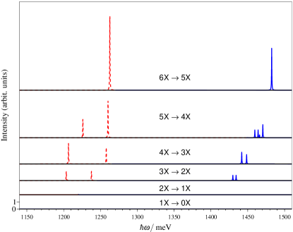
Figure 4: (color online) Ground state emission spectra for a QD with different number of excitons. The high-energy side is shown in blue (solid lines), the low-energy side in red (dashed lines). For the studied system almost no ground state emission is observed for exciton and biexciton. As initial states the ground states with $S^{tot}_{z}=0$ are chosen and the internal electric field is switched off.

In a ground state emission spectrum, without Coulomb interaction, one would observe one line at the high-energy side at $\epsilon^{e}_{p}+\epsilon^{h}_{s}$ and one at $\epsilon^{e}_{s}+\epsilon^{h}_{p}$ on the low-energy side for an initial filling from three to six excitons. With Coulomb interaction, one observes instead of single lines clusters of peaks as shown in Fig. 4. These clusters blue-shift as the number of excitons is increased. The approximate position of the clusters can already be explained by considering only the diagonal elements of the Hamiltonian matrix, see Fig. 5. Note that non-identical envelopes lead to additional interaction terms in comparison to Refs. Hawrylak, 1999; Dekel et al., 2000; Baer et al., 2004. The transition energy $\Delta E^{\text{diag}}_{A\rightarrow B}$ from a many-particle configuration $|A\rangle$ to a configuration $|B\rangle$ is given to a first approximation by Baer et al. (2004)

$$\Delta E^{\text{diag}}_{A\rightarrow B} =\epsilon^{e}_{\bar{e}}+\epsilon^{h}_{\bar{h}}-D^{eh}_{\bar{e}\bar{h}}\;$$ (12)

$$+\sideset{}{}{\sum}_{i\neq\bar{e},\bar{h}}\big{(}D^{ee}_{\bar{e}i}\,n_{i}^{e}-D^{eh}_{\bar{e}i}\,n_{i}^{h}-X^{ee}_{\bar{e}i}\,n_{i}^{e}\big{)}$$

$$+\sideset{}{}{\sum}_{i\neq\bar{e},\bar{h}}\big{(}D^{hh}_{i\bar{h}}\,n_{i}^{h}-D^{eh}_{i\bar{h}}\,n_{i}^{e}-X^{hh}_{i\bar{h}}\,n_{i}^{h}\big{)}\;\;.$$

Here $\bar{e}$ and $\bar{h}$ denote the single-particle states of the electrons and holes, respectively, that are depopulated in the emission process. The index $i$ involves all single-particle states except $\bar{e}$ and $\bar{h}$. The quantity $D^{\lambda\lambda^{\prime}}_{ij}$ stands for the direct Coulomb matrix elements $V^{\lambda\lambda^{\prime}}_{ijji}$, while the exchange matrix elements $X^{\lambda\lambda^{\prime}}_{ij}$ are given by $V^{\lambda\lambda^{\prime}}_{ijij}$. Of course, these exchange terms contribute only if the spin of $\bar{e}$ or $\bar{h}$ agrees with the electron or hole state $i$. The first line of Eq. (12) contains the free particle energies $\epsilon^{e}_{\bar{e}}$ and $\epsilon^{h}_{\bar{h}}$ of the recombining carriers together with the attractive Coulomb interaction matrix element $-D^{eh}_{\bar{e}\bar{h}}$. All terms that stem from the interaction of the electron in state $\bar{e}$ with all the other electrons and holes have been grouped in the second line. Similarly, the third line contains the interaction between the hole labeled with $\bar{h}$ and all the other carriers. Explicitly, one obtains for the high-energy transition of the $3X$ configuration:

$$E^{\text{diag}}_{3X\rightarrow 2X} =\epsilon^{e}_{p}+\epsilon^{h}_{s}-D^{eh}_{ps}$$ (13)

$$+2D^{ee}_{sp}-D^{eh}_{ps}-D^{eh}_{pp}-X^{ee}_{sp}$$

$$+D^{hh}_{ss}+D^{hh}_{sp}-2D^{eh}_{ss}-X^{hh}_{sp}\;\;.$$

Figure 5: (color online) Comparison of QD ground state emission spectra using the CI-approach (solid lines) and the diagonal Hamiltonian (dashed lines) for various multi-exciton transitions. In case of six excitons the two results practically coincide. All data are calculated in the absence of the piezo electric field.

Similarly, one finds from Eq. (12) for the ground state transitions on the high-energy side for more than three excitons:

$$E^{\text{diag}}_{4X\rightarrow 3X} =E^{\text{diag}}_{3X\rightarrow 2X}+\Delta E_{\text{Hartree}}-X^{ee}_{pp}-X^{hh}_{sp}\,,$$ (14)

$$E^{\text{diag}}_{5X\rightarrow 4X} =E^{\text{diag}}_{4X\rightarrow 3X}+\Delta E_{\text{Hartree}}\,,$$

$$E^{\text{diag}}_{6X\rightarrow 5X} =E^{\text{diag}}_{5X\rightarrow 4X}+\Delta E_{\text{Hartree}}\,.\;\;$$

Note that the Hartree-shift $\Delta E_{\text{Hartree}}$, defined by $(D^{ee}_{pp}-D^{eh}_{pp})+(D^{hh}_{ps}-D^{eh}_{ps})$ , would be zero for identical envelopes of electrons and holes. The matrix element $X^{ee}_{pp}$ is given by $V^{ee}_{p_{+}p_{-}p_{+}p_{-}}$. The peaks obtained from the diagonal description provide the approximate position of the clusters calculated by the CI, see Fig. 5. In particular the smaller shift of the $4X$ spectrum relative to the $3X$ spectrum as compared to the shifts involving more excitons is well described in terms of the exchange matrix elements present in the first line of Eq. (14). The corresponding transition energies of the low-energy side can be found by changing $e\leftrightarrow h$ in the equation above.

While the central position of the clusters is well reproduced by the diagonal treatment, the different splitting within each cluster is not explained. A detailed analysis of the states involved in the different emission processes shows that a semi-analytic description of the spectrum is possible. Such a description will be given in the following sections.

VI Semi-Analytic Discussion of the Multi-Exciton Spectra

In the past, optical multi exciton spectra for nitride QDs have only been discussed with selection rules carried over from the InGaAs system. Hohenester et al. (1999); Shi (2002); DeRinaldis et al. (2004) Additionally, the diagonal treatment, which is often suitable for the description of major trends in the InGaAs system Dekel et al. (2000); Franceschetti et al. (2000); Shumway et al. (2001); Bester and Zunger (2003); Ulrich et al. (2005), can in the present case reproduce only the overall position of the clusters, but is by no means sufficient to explain the multiplets. Therefore we will discuss in the following the different multi-exciton spectra of Fig. 4 in detail.

VI.1 $\mathbf{3X\rightarrow 2X}$ Emission spectrum

The ground state emission spectrum with an initial filling of three excitons, is dominated by pairs of lines on the high- and on the low-energy side, see Fig. 6. We will analyze only the low-energy side, as the same line of arguments can be carried out for the high-energy side.

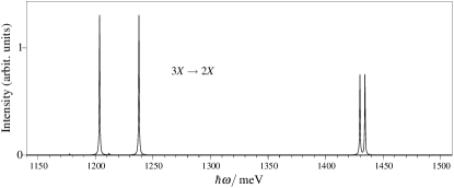
Figure 6: Ground state emission spectrum for an initial filling of three excitons. As initial states the ground states with $S^{tot}_{z}=0$ are chosen.

Due to the spin symmetry we can restrict ourselves to one of the two possible ground states, for which the dominant configuration (according to the CI calculation) is shown in Fig. 7. A linear combination of configuration $|A\rangle$ and $|B\rangle$, enters the $3X$-ground state with the same amplitude but opposite sign. Nevertheless, one can restrict the discussion to either $|A\rangle$ or $|B\rangle$, because they individually produce the same spectrum and possible interference terms in the expansion of the coupling matrix elements appearing in Fermi’s golden rule are zero.

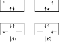
Figure 7: One of the two configurations dominating the three-exciton ground states with $S^{tot}_{z}=0$.

In Fig. 8 configuration $|A\rangle$ is shown together with the $2X$-configuration (in black) that can be reached via the action of $\mathcal{P}_{\text{low}}$. Note that the latter is not an eigenstate of the Hamiltonian. Instead it will be mixed with other states by Coulomb interaction. The predominant contribution to this mixture is shown in Fig. 8 in light grey. Together these two states either form a spin triplet state for the electrons and a spin singlet for the holes ($ts$) or a singlet-singlet ($ss$) state. These $ss$ and $ts$ states are split by the exchange Coulomb matrix element $2X_{sp}^{ee}$ and can both be observed in the spectrum. The oscillator strengths of the corresponding transitions are equal since both final states contain the bright $2X$-exciton state with the same probability amplitude. Along the same line one finds for the high-energy side an approximate splitting of $2X_{sp}^{hh}$ which is, however, considerably smaller. Both splittings are in good agreement with the CI result and explain the dominant peak structure in Fig. 6. The ratio of the peak heights on the low- and the high-energy side is given in terms of the dipole-matrix elements by $d^{eh}_{sp}/d^{eh}_{ps}$.

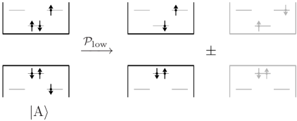
Figure 8: One part of the dominant configuration of the $3X$-ground state characterized by $S_{z}^{e}=+\frac{1}{2}$ and $S_{z}^{h}=-\frac{1}{2}$, together with the $2X$ configuration (in black) that is created by removing the $sp$-exciton via the action of $\mathcal{P}_{\text{low}}$. Additionally the most important dark configuration to which the bright $2X$-state couples via Coulomb interaction is shown in light grey.

VI.2 $\mathbf{4X\rightarrow 3X}$ Emission spectrum

The ground state emission spectrum of $4X$ looks similar to the $3X$ emission spectrum. However, the energetic splitting within the cluster is larger and the oscillator strength of the two lines of the cluster differs from each other. By considering the involved states, we find that the difference can be explained by the fact that the final states are now doublet-doublet ($dd$) and quadruplet-doublet ($qd$) states and no longer simple $ss$ and $ts$ states as in the $3X$ case. The corresponding quadruplet-doublet splitting, which determines the energy difference within the cluster, is larger than the singlet-triplet splitting. Evaluating the contribution of the three different $S_{z}^{\text{tot}}=0$ states, yields an approximate ratio of 5 to 4 for the different oscillator strengths within the cluster and is in good agreement with the CI result.

VI.3 $\mathbf{5X\rightarrow 4X}$ Emission spectrum

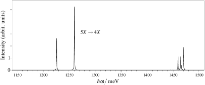
Figure 9: Ground state emission spectrum for an initial filling of five excitons. As initial states the ground states with $S^{tot}_{z}=0$ are chosen.

In contrast to the other multi-exciton spectra, Fig. 9 shows a clear asymmetry and additional lines at the high-energy side of the spectrum.

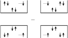
Figure 10: Dominant ground state configuration for five excitons with $S^{tot}_{z}=0$. By flipping all spins a second, degenerate ground state is produced.

One of the $5X$ ground states is depicted in Fig. 10. Taking this as the initial state, the main contribution to the final states for the high-energy side stem from the $6\times 6$ block generated by the configurations schematically represented in Fig. 11. These states have the lowest non-interacting energy amongst those states that can be reached by a removal of one $ps$-exciton from the configurations shown in Fig. 10. Their electronic configuration is given by $2e_{s}2e_{p}1h_{s}3h_{p}$. A similar block with configurations $1e_{s}3e_{p}2h_{s}2h_{p}$ is found for the low-energy transitions. Due to this symmetry one would expect the same number of lines on the high- and on the low-energy side of the spectrum. This expectation is fulfilled for all but the $5X\rightarrow 4X$ transitions.

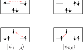
Figure 11: (color online) Main contribution to the final states of the high-energy side of the $5X\rightarrow 4X$ transition with classification $S^{\text{tot}}_{z}=0$ and, assuming full angular momentum conservation, $l^{\text{tot}}_{z}=0$. The arrow between electrons or holes indicates that additional states can be derived from the displayed configuration by flipping the spins of the connected carriers simultaneously. This way one can create four different states from the first configuration and two from the second one.

By combining the first four states $|\psi_{1,\ldots,4}\rangle$ in Fig. 11 one can form ss, st, ts and tt spin states. The last two states $|\psi_{5,6}\rangle$ in Fig. 11 allow the formation of an st and ss state. While the electrons of the first four states always occupy both $p_{+}$ and $p_{-}$, they occupy only the $p_{-}$ state in the last two configurations. Therefore one expects that the energy of the $ss$ state formed by the states $\psi_{1}$ to $\psi_{4}$ differs from the energy of the eigenstate created by combining $\psi_{5}$ and $\psi_{6}$. By the same token one expects two different energies for the two possible $st$-states. Therefore six different energies can be expected. On the high energy side of the spectrum four lines are clearly visible and another two may be identified on the left side of the cluster. For the low-energy side, however, only two lines can be observed.

To obtain further insight, we construct the Hamiltonian matrix generated from the states $\{|\psi_{i}\rangle\}^{6}_{i=1}$ and block-diagonalize it by transforming to spin-eigenstates. This way one obtains four subblocks:

$$H_{\text{ts}} =-\frac{3}{2}\;, \qquad H_{\text{{ss}}}=\frac{1}{2}\begin{pmatrix}-1&t\\ t&1\end{pmatrix}\;,$$ (15)

$$H_{\text{st}} =-2\tilde{t}\underline{\underline{1}}-H_{ss}\;, \qquad H_{\text{tt}}=-2\tilde{t}-\frac{3}{2}\;,\;\;\;\;$$ (16)

where we introduced the dimensionless parameters $t=2\sqrt{2}X^{eh}_{pp}/X^{ee}_{pp}$ and $\tilde{t}=X^{eh}_{pp}/X^{ee}_{pp}$ and measured all energies in units of $X^{ee}_{pp}$ relative to $E^{\text{diag}}+\tilde{t}+\frac{1}{2}$ with $E^{\text{diag}}$ being the energy of the configurations in the diagonal approximation. The six eigenvalues of these blocks are $E_{\text{ts}}=-\frac{3}{2}$, $E_{\text{ss}}=\pm\frac{1}{2}\sqrt{1+t^{2}}$, $E_{\text{st}}=-2\tilde{t}\mp\frac{1}{2}\sqrt{1+t^{2}}$, and $E_{\text{tt}}=-2\tilde{t}-\frac{3}{2}$. From these expression one can read off that the st and tt spectrum is shifted by $-2\tilde{t}$ relative to the $ss$ and $ts$ spectrum, respectively.

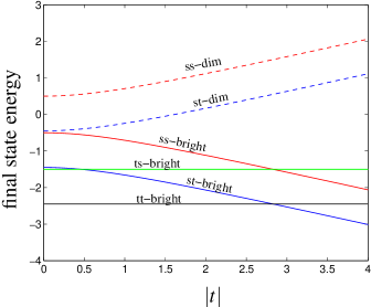
Figure 12: (color online) Energies of the final states involved in the high-energy transition measured in units of $X^{ee}_{pp}$ relative to $E^{\text{diag}}+\tilde{t}+\frac{1}{2}$ as a function of the dimensionless parameter $t=2\sqrt{2}{X^{eh}_{pp}}/{X^{ee}_{pp}}$ for fixed $\tilde{t}\approx 0.47$. The labeling refers to the spin configuration of the final states and whether the states are ’bright’ or ’dim’.

In order to obtain the corresponding oscillator strengths of the transitions, one has to calculate the matrix elements $|\langle 4X,i|\mathcal{P}_{\text{high}}|5X,\text{gs}\rangle|^{2}$, where $|4X,i\rangle$ denotes the $i$-th eigenstate of the four exciton problem and $|5X,\text{gs}\rangle$ refers to the ground states schematically shown in Fig. 10 of the five exciton problem. Because the eigenstate within the one-dimenstional subspaces of the ts- and tt-states is not affected by a varied parameter $t$, the oscillator strength does not depend on the value of $t$. In contrast, the heights of the ss- and st-lines depend strongly on $t$ as the amplitude of the different states in the linear combination varies with $t$. Denoting the eigenstates of $H_{\text{ss}}$ with $(\alpha_{i},\beta_{i})^{t}$ the oscillator strength $\Sigma$ of the ss transition is given by

$$\Sigma=|d^{eh}_{ps}|^{2}\;\Big{|}\frac{\alpha_{i}}{\sqrt{2}}+\frac{\beta_{i}}{2}\Big{|}^{2}\;\;.$$ (17)

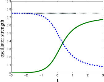
Figure 13: (color online) Oscillator strengths, shown in green (solid line) and blue (dashed line), of the two $ss$ transitions as a function of the dimensionless parameter $t$. A clear redistribution of oscillator strength from one to the other transition is visible. The total oscillator strength, red (dotted line), however, remains unchanged. The same behavior is found for the st transition.

A similar analysis can be performed for the $st$ transition. In this case one finds

$$\Sigma=|d^{eh}_{ps}|^{2}\;\Big{|}\frac{\alpha_{i}}{2}-\frac{\beta_{i}}{\sqrt{2}}\Big{|}^{2}\;\;$$ (18)

for the oscillator strength. As $H_{\text{ss}}$ and $H_{\text{st}}$ have the same eigenvectors and if $v=(\alpha,\beta)^{t}$ is an eigenvector, so is $v^{\prime}=(-\beta,\alpha)^{t}$, one finds for the $st$-transitions the same dependency of the oscillator strength as for the $ss$ transition. For the analysis of the low-energy cluster, only the labels $e\leftrightarrow h$ have to be changed in all the derived equations.

The dependence of the transition energies and the oscillator strengths on the parameter $t$ are depicted in Fig. 12 and Fig. 13, respectively. For above discussed QD example, one obtains $t\approx-1.2$ for the high-energy side and $t\approx-2.8$ for the low energy side. Therefore we expect from Fig. 13 that one will only be able to observe in the spectrum one of the $ss$ and one of the $st$ lines in addition to the $ts$ and $tt$ line. This explains the four clearly visible lines in Fig. 9 of the high energy side. In contrast, for the low-energy side only two peaks are visible. This can be traced back to the fact that one has in this case $X^{eh}_{pp}\approx X^{ee}_{pp}$ or $t\approx 2\sqrt{2}$. According to Fig. 12 this means that the $ss$ and $st$ as well as $ts$ and $tt$ have almost identical transition energies. As a consequence of this degeneracy only two distinct lines can be observed on the low-energy side of the spectrum.

VI.4 $\mathbf{6X\rightarrow 5X}$ Emission spectrum

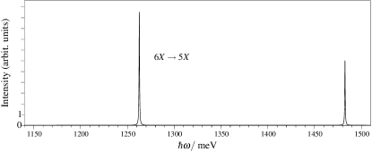
Figure 14: Ground state emission spectrum for an initial filling of six excitons.

In the case of two shells for each type of carrier, the QD is completely filled with six excitons and there is only one ground state possible. By removing one $sp$-exciton or one $ps$-exciton from this configuration, we find that the possible final states are exactly those for the $0X\rightarrow 1X$ transitions, only that the occupied sites in the $0X\rightarrow 1X$ problem are now the unoccupied ones. Therefore the $6X\rightarrow 5X$ emission spectrum, see Fig. 14, is very similar to the $0X\rightarrow 1X$ absorption spectrum, with the main difference being that the lines are shifted due to the interaction with the ’background’ carriers.

VII Influence of the Built-In Field

Nitride QDs grown along the $c$-axis are characterized by the presence of a strong internal electrostatic field which has a component stemming from the spontaneous polarization and a part generated by strain. When this field is included in the calculation of the single-particle properties, the electron and hole wave functions are spatially separated from each other which leads to a reduction of the oscillator strength. Andreev and O’Reilly (2001); DeRinaldis et al. (2002); Schulz et al. (2006) Furthermore the single-particle gap and the Coulomb matrix elements are altered. The resulting multi-exciton spectra with and without the inclusion of the built-in field are compared in Fig. 15.

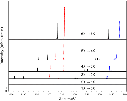
Figure 15: (color online) Ground state emission spectra for the smaller QD ($d=4.5$ nm and $h=1.6$ nm)with (solid lines) and without (dashed lines) the inclusion of the internal field. Different number of excitons with $S^{tot}_{z}=0$ are chosen as initial states. For the studied system almost no ground state emission is observed for the exciton and biexciton.

The reduced oscillator strength and the overall red-shift of the spectra due to the QCSE are clearly visible. In addition to these results of the modified single-particle properties, we find a stronger shift of the lines with increasing number of excitons in the presence of the internal field. This is another result of the strong separation of the electron and hole wave functions which also introduces Hartree-shifts in the spectrum. Indeed, if the diagonal approximation is applied as outlined in Section V.3, one obtains again the position of the cluster to a good approximation. Another difference can be observed in the $5X\rightarrow 4X$ spectrum: The number lines changes in the presence of the intrinsic field. Since for all other excitonic populations the spectra are only altered quantitatively this is a rather surprising result. But this is resolved by noting that the situation without the intrinsic field is rather special as one had $X^{eh}_{pp}\approx X^{ee}_{pp}$. Including the built-in field leads to a significant deviation of the two matrix elements and henceforth to a clear splitting of the previously degenerate lines.

VIII Multi-Exciton Emission for a Larger Quantum Dot

In order to give a more representative overview, we additionally investigate a larger QD with diameter $d=5.7\text{nm }$ and height $h=2.3\text{nm }$. It turns out, that in this case the energetic order of the two energetically lowest hole levels is reversed in the presence of the internal electrostatic field. A schematic picture of this situation is shown in Fig. 16. In the absence of the built-in field, one still has the ‘usual’  order with the $s$-shell being lower in energy than the $p$-shell. Hence, the spectrum looks similar to those previously discussed and is here therefore omitted. However, in the presence of the built-in field the two-fold degenerate $p$-shell constitutes the hole ground states and has, according to the symmetry considerations of Section III, non-vanishing dipole matrix elements with the electron ground state. This is in agreement with recent $\mathbf{k}\cdot\mathbf{p}$ calculations Bagga et al. (2005) and experimental results for CdSe QDs Nirmal et al. (1995) grown in the wurtzite phase. As an immediate consequence the excitonic and biexcitonic ground state is bright. However, the corresponding $d^{eh}_{sp}$ dipole-matrix elements are strongly reduced in comparison with the smaller QD due to the stronger separation of the electron and hole wave function in this larger structure.

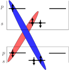
Figure 16: (color online) Schematic representation of a three exciton configuration. The light (red) and dark (blue) shaded areas connect the carriers that will lead to a emission at the low- and high-energy side of the spectrum, respectively.

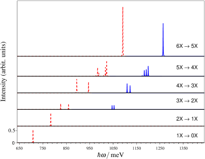
Figure 17: (color online) Emission spectra for a larger quantum dot (d = 5.7 nm and h = 2.3 nm) with different number of excitons and in the presence of the internal field. For the emission of each multi-exciton complex the high-energy side is shown in blue (solid lines), the low-energy side in red (dashed lines). Due to the reversed level structure for the holes a ground state emission is observed for exciton and biexciton. As initial states the ground states with $S^{\text{tot}}_{z}=0$ are chosen.

The resulting multi-exciton spectra are shown in Fig. 17. In contrast to the intuitive picture in which first the states with lowest single-particle energy are occupied, a strong population of the hole $s$-shell for more than one exciton is found. The ground states are therefore not given by those states with lowest non-interacting energy. This is already confirmed by a calculation that contains only the Hartree Coulomb terms and can qualitatively be explained as follows: The attraction between the electron and hole being in their respective $s$-shells is stronger than the attraction in the case of $s$- and $p$-shell carriers. Therefore it can compensate the higher single-particle energy of the hole in the $s$-shell. This leads already for the biexciton to an occupation of the hole $s$-shell. However, an additional promotion of the other hole is not favored in this case because the increase in energy due to the stronger repulsive interaction between the holes in their $s$-shell is higher than the energy reduction due to the stronger attraction between $s$-electrons and $s$-holes. As a consequence, the $s$- and $p$-shell for the holes are equally populated in the biexciton ground state. Therefore the biexcitonic line has approximately the same oscillator strength as the excitonic one.

From three excitons on, the ground states are dominated by configurations in which both the $s$-shell for electrons and the $s$-shell for holes are fully populated. As a consequence, one obtains qualitatively the same spectra as in the case of the smaller dot with the ‘normal’  order of the shells. However, one finds that the oscillator strengths are strongly reduced in the larger system and that the Hartree shifts are even more pronounced, due to the strong separation of electron and hole wave functions.

IX Conclusion

In this work we have investigated the electronic and optical properties of lens-shaped InN/GaN QDs. Employing a tight-binding model where the weak crystal-field splitting and spin-orbit coupling for the system studied here are neglected, we found an exactly degenerate single-particle $p$-shell. This degeneracy originates from the $C_{3v}$-symmetry of the underlying wurtzite lattice. This result is in particular intriguing in view of recent discussions in the literature about the $p$-shell degeneracy in zinc-blende QDs. Based on the microscopically determined single-particle wave functions, the dipole and Coulomb matrix elements were evaluated. These matrix elements served as input parameters for configuration interaction calculations and allowed the determination and further analysis of optical properties. Our prediction of dark exciton and biexciton ground state for small dots is confirmed by symmetry considerations. In contrast to other III-V material systems, the emission from nitride-based QDs is dominated by ’skew’ excitons, so that completely different multi-exciton spectra arise. For larger QDs, we found that the strong internal electric built-in field can reverse the energetic order of the hole states, which results in a bright exciton and biexciton ground state. However, the oscillator strength is strongly reduced in these structures due to the quantum confined Stark effect. By restricting the analysis to the energetically lowest shells, a semi-analytic description of the optical properties was possible, leading to a deeper insight into the origin of the various emission lines.