Family of Commuting Operators for the Totally Asymmetric Exclusion Process

Abstract

The algebraic structure underlying the totally asymmetric exclusion process is studied by using the Bethe Ansatz technique. From the properties of the algebra generated by the local jump operators, we explicitly construct the hierarchy of operators (called generalized hamiltonians) that commute with the Markov operator. The transfer matrix, which is the generating function of these operators, is shown to represent a discrete Markov process with long-range jumps. We give a general combinatorial formula for the connected hamiltonians obtained by taking the logarithm of the transfer matrix. This formula is proved using a symbolic calculation program for the first ten connected operators.

Keywords: ASEP, Algebraic Bethe Ansatz.

Pacs numbers: 02.30.Ik, 02.50.-r, 75.10.Pq.

1 Introduction

The Asymmetric Simple Exclusion Process (ASEP) is a driven lattice gas of particles that hop on a lattice and interact through hard-core exclusion. Originally, the ASEP was proposed as a minimal model in one-dimensional transport phenomena with geometric constraints, such as hopping conductivity, motion of RNA templates and traffic flow. The exclusion process displays a rich phenomenological behaviour and its relative simplicity has allowed to derive many exact results in one dimension. For these reasons, the ASEP has become one of the major models in the field of interacting particle systems both in the mathematical and the physical literature and plays the role of a paradigm in non-equilibrium statistical mechanics (for reviews, see e.g., Spohn 1991, Derrida 1998, Schütz 2001).

It has been shown that the evolution operator (or Markov matrix) of the exclusion process can be mapped into a non-hermitian Heisenberg spin chain of the XXZ type (Gwa and Spohn, 1992; Essler and Rittenberg 1996). This mapping allows the use of the techniques of integrable systems such as the coordinate Bethe Ansatz (for a review see, e.g., Golinelli and Mallick, 2006b). Spectral information about the evolution operator (Dhar 1987; Gwa and Spohn 1992; Schütz 1993; Kim 1995; Golinelli and Mallick 2005) and large deviation functions (Derrida and Lebowitz 1998) can be derived with the help of coordinate Bethe Ansatz. Besides, using the more elaborate algebraic Bethe Ansatz technique, the eigenstates of the Markov matrix can be represented as Matrix Product states over finite dimensional quadratic algebra (Golinelli and Mallick, 2006a). The algebraic Bethe Ansatz also plays a fundamental role in the derivation of the Bethe equations for ASEP with open boundaries (de Gier and Essler, 2005, 2006).

The aim of the present work is to explore the algebraic properties of the totally asymmetric exclusion process (TASEP) that stem from the algebra generated by the local jump operators that build the Markov matrix. The algebraic Bethe Ansatz technique allows to construct a hierarchy of generalized hamiltonians that contain the Markov matrix and commute with each other. The generating operator for this family, called the transfer matrix, defines therefore a commuting family of operators that can be simultaneously diagonalized. We derive, using the local jump operators algebra, explicit formulae for the transfer matrix and the generalized hamiltonians and characterize their action on the configuration space. These generalized hamiltonians are non-local because they act on non-connected bonds of the lattice. However, connected operators are generated by taking the logarithm of the transfer matrix. We study these connected operators and give an explicit formula for them.

The outline of this work is as follows : in Section 2, we describe the basic algebraic properties of the totally asymmetric exclusion process and define the associated algebra. In Section 3, we give explicit formulae for the transfer matrix and for the generalized hamiltonians that commute with the Markov matrix $M$. In particular, we show that the transfer matrix can be interpreted as a discrete time Markov process and we describe the non-local actions of the generalized hamiltonians. In Section 4, we study the connected operators obtained by taking the logarithm of the transfer matrix and propose a conjectured general formula for these local operators. The actions of these operators are described explicitly. Some mathematical proofs are given in the appendices.

2 Algebraic properties of the TASEP

2.1 Definition of the model

The simple exclusion process is a continuous-time Markov process (i.e., without memory effects) in which indistinguishable particles hop from one site to another on a discrete lattice and obey the exclusion rule which forbids to have more than one particle per site. In this work, we shall study the case of particles hopping on a periodic 1-d ring (see figure 1) with $L$ sites labelled $i=1,\dots,L$ (sites $i$ and $i+L$ are identical due to periodic boundary conditions). The particles move according to the following dynamics: during the time interval $[t,t+dt]$, a particle on a site $i$ jumps with probability $dt$ to the neighboring site $i+1$, if this site is empty. This model is called ‘totally asymmetric’ because the particles can jump only in one direction. The exclusion rule forbids particles to overtake each other and their ordering remains unchanged. Moreover, as the system is closed, the number of particles is constant.

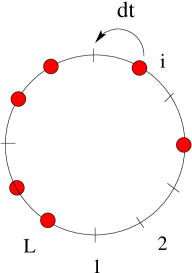
Figure 1: The totally asymmetric exclusion process on a ring. Sites are labelled from 1 to $L$; a particle jumps with probability $dt$ to the neighbouring forward site if this site is vacant.

The state of a site $i$ is encoded in a boolean variable $\tau_{i}$, where $\tau_{i}=1$ if $i$ is occupied and $\tau_{i}=0$ otherwise. The two-dimensional state space of the site $i$ is noted $V_{i}$ (we have $V_{i}=\mathbb{C}^{2}$) and its basis is given by $(|1_{i}\rangle,\ |0_{i}\rangle)$. A configuration $C$ of the system of $L$ sites is written as

$$C=|\tau_{1},\tau_{2}\dots\tau_{L}\rangle\,.$$ (1)

The state space $\mathcal{H}_{L}$ of the ring is therefore a $2^{L}$ dimensional vector space given by

$$\mathcal{H}_{L}=V_{1}\otimes V_{2}\otimes\dots\otimes V_{L}\,.$$ (2)

Due to the conservation of the number $n$ of particles, $\mathcal{H}_{L}$ splits into invariant spaces ${\mathcal{H}}_{L}^{(n)}$ of dimension $L!/[n!(L-n)!]$, characterized by $\sum_{i=1}^{n}\tau_{i}=n$.

The probability distribution of the system at time $t$ can be represented as a vector $\psi(t)\in\mathcal{H}_{L}$, where the component $\psi_{C}(t)$ is the probability of being in the configuration $C$ at time $t$. The vector $\psi(t)$ evolves according to the master equation

$$\frac{d\psi(t)}{dt}=M\psi(t)\,,$$ (3)

where $M$ is a $2^{L}\times 2^{L}$ Markov matrix acting on $\mathcal{H}_{L}$. For $C\neq C^{\prime}$, $M(C^{\prime},C)$ is the transition rate from configuration $C$ to configuration $C^{\prime}$: it is equal to 1 if $C^{\prime}$ is obtained from $C$ by an allowed jump of a particle, and 0 otherwise. The diagonal elements are negative and $-M(C,C)$ is the exit rate from $C$, i.e., the number of allowed jumps from $C$. The sums over columns of $M$ vanish, $\sum_{C^{\prime}}M(C^{\prime},C)=0$. This property ensures probability conservation : $\sum_{C}\psi_{C}(t)=\sum_{C}\psi_{C}(0)=1$.

In the case of the TASEP on a periodic ring, sums over rows of $M$ also vanish. This implies that the stationary probability, obtained for $t\to\infty$, is uniform over each subspace ${\mathcal{H}}_{L}^{(n)}$.

2.2 The algebra of jump matrices

The Markov matrix can be written as

$$M=\sum_{i=1}^{L}M_{i}\,,$$ (4)

where the local jump operator $M_{i}$ represents the contribution to the dynamics of jumps from the site $i$ to $i+1$. Thus, the action of the $2^{L}\times 2^{L}$ operator $M_{i}$ affects only the sites $i$ and $i+1$ and is non-zero only if $\tau_{i}=1$ and $\tau_{i+1}=0$ :

$$M_{i}|\tau_{1}\dots 1,0\dots\tau_{L}\rangle = |\tau_{1}\dots 0,1\dots\tau_{L}\rangle-|\tau_{1}\dots 1,0\dots\tau_{L}\rangle\ ,$$ (5)

$$M_{i}|\tau_{1}\dots\tau_{i},\tau_{i+1}\dots\tau_{L}\rangle = 0,\ \ \ \ \mbox{if}\ \tau_{i}=0\ \mbox{or}\ \tau_{i+1}=1\,.$$ (6)

The operator $M_{L}$ corresponds to jumps from site $L$ to 1 (the site $L+1$ is identical to the site 1 because of the periodic boundary conditions).

Using this definition of the local jump operators, it can be verified that the $M_{i}$ satisfy the following relations :

$$M_{i}^{2} = -M_{i},$$ (7)

$$M_{i}\ M_{i+1}\ M_{i}=M_{i+1}\ M_{i}\ M_{i+1} = 0,$$ (8)

$$\left[M_{i},M_{j}\right] = 0\ \ \ \mathrm{if}\ |i-j|>1.$$ (9)

As we consider a periodic system, we use the convention $M_{L+1}\equiv M_{1}$ in the above relations. We emphasize that $[M_{L},M_{1}]\neq 0$ and $M_{1}M_{L}M_{1}=M_{L}M_{1}M_{L}=0$.

The algebra generated by the $M_{i}$ operators will be called here the TASEP algebra. We remark that the $M_{i}$ operators can be obtained as a limit of the Temperley-Lieb algebra generators. We shall call, by definition, a word, any product of the $M_{i}$’s; any element of the algebra can be written as a linear combination of words. The length of a word is the minimal number of operators $M_{i}$ required to write it.

Each word acts on the configuration space $\mathcal{H}_{L}$ and can be described as a series of jumps. For example, the word $M_{1}M_{2}$ describes a jump of a particle from site 2 to 3, followed by a jump of another particle from site 1 to the site 2; the action of $M_{1}M_{2}$ on a configuration vanishes unless $\tau_{1}=1,\,\tau_{2}=1,\,\tau_{3}=0$ and we have

$$M_{1}M_{2}|1,1,0,\tau_{4}\dots\tau_{L}\rangle=|0,1,1,\tau_{4}\dots\tau_{L}\rangle-|1,0,1,\tau_{4}\dots\tau_{L}\rangle\,.$$ (10)

Similarly, the word $M_{2}M_{1}$ represents a jump of a particle from site 1 to 2 followed by a jump of the same particle from 2 to 3 :

$$M_{2}M_{1}|1,0,0,\tau_{4}\dots\tau_{L}\rangle=|0,0,1,\tau_{4}\dots\tau_{L}\rangle-|0,1,0,\tau_{4}\dots\tau_{L}\rangle\,.$$ (11)

Clearly, $M_{1}$ and $M_{2}$ do not commute because the jumps on two adjacent sites are not independent.

2.3 Ring-ordered product of jump matrices

We define here the ring-ordered product of jump matrices which will be used in the following sections.

The ring-ordered product $\mathcal{O}\left(\right)$ acts on words of the type

$$W=M_{i_{1}}M_{i_{2}}\dots M_{i_{k}}\,\hbox{ with }\,1\leq i_{1}<i_{2}<\dots<i_{k}\leq L\,,$$ (12)

by changing the positions of matrices that appear in $W$ according to the following rules :

(i) If $i_{1}>1$ or $i_{k}<L$, we define $\mathcal{O}\left(W\right)\ =W$. The word $W$ is well-ordered.

(ii) If $i_{1}=1$ and $i_{k}=L$, we first write $W$ as a product of two blocks, $W=AB$, such that $B=M_{b}M_{b+1}\dots M_{L}$ is the maximal block of matrices with consecutive indices that contains $M_{L}$, and $A=M_{1}M_{i_{2}}\dots M_{i_{a}}$, with $i_{a}<b-1$, contains the remaining terms. We then define

$$\mathcal{O}\left(W\right)=\mathcal{O}\left(AB\right)=BA=M_{b}M_{b+1}\dots M_{L}M_{1}M_{i_{2}}\dots M_{i_{a}}\,.$$ (13)

(iii) The previous definition makes sense only for $k<L$. Indeed, when $k=L$, we have $W=M_{1}M_{2}\dots M_{L}$ and it is not possible to split $W$ in two different blocks $A$ and $B$. For this special case, we define

$$\mathcal{O}\left(M_{1}M_{2}\dots M_{L}\right)\ =|1,1,\dots,1\rangle\langle 1,1,\dots,1|\,,$$ (14)

which is the projector on the ‘full’ configuration with all sites occupied.

The ring-ordering $\mathcal{O}\left(\right)$ is extended by linearity to the vector space spanned by words of the type described above.

Let us give some examples. For $k=0$ or 1, the ring-ordered product acts trivially: $\mathcal{O}\left(1\right)=1$ and $\mathcal{O}\left(M_{i}\right)=M_{i}$. For $k=2$ , we have $\mathcal{O}\left(M_{i}M_{j}\right)=M_{i}M_{j}$ when $1\leq i<j\leq L$; however, for the special case when $i=1$ and $j=L$, $\mathcal{O}\left(M_{1}M_{L}\right)=M_{L}M_{1}$.

The ring-ordered product embodies the periodic boundary conditions. On a ring, the natural order between integers is not valid. Indeed, $M_{L}$ and $M_{1}$ act as neighbouring bonds and site $L$ should be viewed as being ’behind’ site 1, just as site 1 is behind site 2. The ring-order product restores the correct order on a ring and allows to construct operators that are translation invariant. For example, for $L=3$, the operator $U=M_{1}M_{2}+M_{2}M_{3}+M_{1}M_{3}$ is not well-ordered and does not commute with translations. But, $\mathcal{O}\left(U\right)=M_{1}M_{2}+M_{2}M_{3}+M_{3}M_{1}$ is well-ordered and does commute with translations. Finally, we remark that when a ring-ordered product acts on a configuration, each particle advances by at most one lattice unit : indeed, because terms such as $M_{i+1}M_{i}$ do not appear in a ring-ordered product, no particle can perform multiple jumps.

3 Transfer matrix and generalized hamiltonians

The algebraic Bethe Ansatz is a method for diagonalizing the hamiltonian of integrable models (for a review, see, e.g., Korepin et al. 1993; for a pedagogical introduction, see, e.g., Nepomechie 1999). This technique can be applied to the Markov matrix $M$ of the TASEP (Golinelli and Mallick, 2006b). The key step is to construct a family of transfer matrices, $t(\lambda)$, which act on the configuration space $\mathcal{H}_{L}$. For any value $\lambda$ and $\nu$ of the spectral parameter, we have

$$[t(\lambda),t(\nu)]=0\,.$$ (15)

Thus, the operators $t(\lambda)$ form a one-parameter family of commuting operators which depend on a real number $\lambda$, called the spectral parameter. This family contains the Markov matrix $M$ as will be shown below. Therefore, all the $t(\lambda)$’s share with $M$ a common eigenvector basis independent of $\lambda$. For the TASEP, these eigenvectors are determinants of matrices involving the roots of the Bethe equations and the corresponding eigenvalues are functions of $\lambda$ (see e.g., Golinelli and Mallick 2006b for an explicit formula).

The transfer matrix $t(\lambda)$ is a polynomial in $\lambda$ of degree $L$ : we can thus define $H_{1},H_{2},\dots H_{L}$ as follows

$$t(\lambda)=t(0)\ \left(1+\sum_{k=1}^{L}\lambda^{k}H_{k}\right)\ .$$ (16)

The $H_{k}$ operators are $2^{L}\times 2^{L}$ matrices acting on the configuration space $\mathcal{H}_{L}$. The $H_{k}$’s will be called ‘generalized hamiltonians’ by analogy with quantum spin systems (Arnaudon et al. 2005). As the $H_{k}$’s are derivatives of $t(\lambda)$, they also commute with each other :

$$[H_{k},t(\lambda)]=0,\ \ \ \ [H_{j},H_{k}]=0$$ (17)

for all $j$, $k$ and $\lambda$. More generally, any operator generated from $t(\lambda)$, or equivalently from the generalized hamiltonians, belongs to the same commuting family.

The above considerations are familiar in the framework of algebraic Bethe Ansatz. In Appendix A, we explain how the transfer matrix can be constructed using this method.

3.1 Expressions of the $H_{k}$’s

In this section we describe our results which are specific to the TASEP and give explicit formulae for the generalized hamiltonians $H_{k}$. The calculations leading to these expressions are carried out in detail in Appendix B.

The $t(0)$ operator appearing in equation (16) is the translation operator on the ring and is defined as

$$t(0)|\tau_{1},\tau_{2},\dots,\tau_{L}\rangle=|\tau_{2},\dots,\tau_{L},\tau_{1}\rangle\ .$$ (18)

The operator $H_{1}$ given by

$$H_{1}=t^{\prime}(0)/t(0)=\sum_{i=1}^{L}M_{i}=M\,,$$ (19)

is precisely the Markov matrix $M$ which thus belongs to the commuting family generated by $t(\lambda)$.

All the $H_{k}$’s can be explicitly calculated. By using the “ring-ordered product” defined in section 2.3, we find in Appendix B that for $1\leq k\leq L$,

$$H_{k}=\sum_{1\leq i_{1}<i_{2}<\dots<i_{k}\leq L}\mathcal{O}\left(M_{i_{1}}M_{i_{2}}\dots M_{i_{k}}\right)\ .$$ (20)

In particular, we have

$$H_{2}=\sum_{1\leq i<j\leq L}\ \mathcal{O}\left(M_{i}M_{j}\right)\ ,$$ (21)

and according to equation (14),

$$H_{L}\ =|1,1,\dots,1\rangle\langle 1,1,\dots,1|\ .$$ (22)

For $k<L$, all the terms in $H_{k}$ are products of $k$ jump matrices which, because of ring-ordering, correspond to $k$ different particles jumping simultaneously one step forward. Thus, $H_{k}$ has a non-vanishing action only on configurations with at least $k$ particles.

In the case with $L=4$, for example, the generalized hamiltonians are given by

$$H_{1} = M_{1}+M_{2}+M_{3}+M_{4}=M\ ,$$ (23)

$$H_{2} = M_{1}M_{2}+M_{2}M_{3}+M_{3}M_{4}+M_{4}M_{1}+M_{1}M_{3}+M_{2}M_{4}\ ,$$ (24)

$$H_{3} = M_{1}M_{2}M_{3}+M_{2}M_{3}M_{4}+M_{3}M_{4}M_{1}+M_{4}M_{1}M_{2}\ .$$ (25)

Using Eqs. (16) and (20), we conclude that the generating function of the $H_{k}$ is given by

$$t_{g}(\lambda)=\frac{t(\lambda)}{t(0)}=1+\sum_{k=1}^{L}\lambda^{k}H_{k}=\mathcal{O}\left(\prod_{i=1}^{L}(1+\lambda M_{i})\right)\,.$$ (26)

Although the operator $H_{1}$ is the Markov matrix $M$ of the TASEP, we emphasize that when $k\geq 2$, $H_{k}$ cannot be interpreted as a Markov matrix because it contains negative non-diagonal matrix elements. However, we shall now prove that the matrix $t(\lambda)$ is the Markov matrix of a discrete time process when $0\leq\lambda\leq 1$.

3.2 Action of the transfer matrix on a given configuration

We describe now the action of $t(\lambda)$ on a given configuration $|\tau_{1},\tau_{2},\dots,\tau_{L}\rangle$. Using equation (26), we observe that

$$t_{g}(\lambda)|\tau_{1},\tau_{2},\dots,\tau_{L}\rangle=\mathcal{O}\left(\prod_{\stackrel{{\scriptstyle i=1}}{{\tau_{i}=1}}}^{L}(1+\lambda M_{i})\right)|\tau_{1},\tau_{2},\dots,\tau_{L}\rangle\,,$$ (27)

where the product runs only over occupied sites. This expression shows that the action of $t_{g}(\lambda)$ is factorized block by block. We consider first the simple block $|01^{p}\rangle$ (the notation $|01^{p}\rangle$ means that a hole is followed by $p$ particles). We have

$$t(\lambda)|01^{p}\rangle=t_{g}(\lambda)|1^{p}0\rangle=(1+\lambda M_{1})\ldots(1+\lambda M_{p})|1^{p}0\rangle=\sum_{k=0}^{p}f_{k,p}|1^{k}01^{p-k}\rangle\,,$$

$$\hbox{ with }f_{0,p}=\lambda^{p}\,\hbox{ and }\,f_{k,p}=(1-\lambda)\lambda^{p-k}\hbox{ for }1\leq k\leq p\,.$$ (28)

More generally, for a configuration $C$ of the form $|0^{q_{1}}1^{p_{1}}0^{q_{2}}1^{p_{2}}\dots 0^{q_{s}}1^{p_{s}}\rangle$ with $p_{i},q_{i}\geq 1$, we obtain

$$t(\lambda)C=t_{g}(\lambda)|0^{q_{1}-1}1^{p_{1}}\dots 0^{q_{s}}1^{p_{s}}0\rangle=$$ (29)

$$|0^{q_{1}-1}\rangle\otimes\left(\sum_{k_{1}=0}^{p_{1}}f_{k_{1},p_{1}}|1^{k_{1}}01^{p_{1}-k_{1}}\rangle\right)\otimes|0^{q_{2}-1}\rangle\otimes\ldots$$

$$\otimes\left(\sum_{k_{s}=0}^{p_{s}}f_{k_{s},p_{s}}|1^{k_{s}}01^{p_{s}-k_{s}}\rangle\right)\,.$$

Except for the full configuration $|1^{L}\rangle$ for which $t(\lambda)|1^{L}\rangle=t_{g}(\lambda)|1^{L}\rangle=(1+\lambda^{L})\ |1^{L}\rangle$ and the void configuration $|0^{L}\rangle$ for which $t(\lambda)\ |0^{L}\rangle=t_{g}(\lambda)\ |0^{L}\rangle=|0^{L}\rangle$, any configuration $C$ has at least one particle and one hole. By using the translation operator $t(0)$ that commutes with $t(\lambda)$, it is possible to bring $C$ to a form to which equation (29) can be applied.

We notice that $t(1)$ is the identity operator. Consequently $t_{g}(1)$ is the forward translation operator, $t_{g}(1)=t(0)^{-1}$.

We illustrate these results with an example of 3 particles on a ring of 5 sites:

$$t(\lambda)\ |10101\rangle=t_{g}(\lambda)\ |01011\rangle=$$ (30)

$$(1-\lambda)^{2}\ |01011\rangle+\lambda(1-\lambda)\ |00111\rangle+\lambda(1-\lambda)^{2}\ |11010\rangle$$

$$+\lambda^{2}(1-\lambda)\ |10110\rangle+\lambda^{2}(1-\lambda)\ |11001\rangle+\lambda^{3}\ |10101\rangle\ .\,\,\,\,$$

By considering the action of the operators $t(\lambda)$ and $t_{g}(\lambda)$, we remark that for $0\leq\lambda\leq 1$, $f_{k,p}\geq 0$ and that $\sum_{k}f_{k,p}=1$. The quantities $f_{k,p}$ can thus interpreted as probabilities. The operators $t(\lambda)$ and $t_{g}(\lambda)$ are then Markov matrices of discrete time exclusion processes with parallel dynamics, in which different holes can jump simultaneously through clusters of particles.

With $t(\lambda)$, a hole located on the left of a cluster of $p$ particles can jump a distance $k$ in the forward direction, $1\leq k\leq p$, with probability $\lambda^{p-k}(1-\lambda)$. The probability that this hole does not jump at all is $\lambda^{p}$.

With $t_{g}(\lambda)$, a hole located on the right of a cluster of $p$ particles can jump a distance $k$ in the backward direction, with probability $\lambda^{k}(1-\lambda)$ for $1\leq k<p$, and with probability $\lambda^{p}$ for $k=p$. The probability that this hole does not jump at all is $1-\lambda$.

The $t_{g}(\lambda)$ Markov process is equivalent to a 3-D anisotropic percolation model and a 2-D five-vertex model (Rajesh and Dhar 1998). It is also an adaptation on a periodic lattice of the ASEP with a backward-ordered sequential update (Rajewsky et al. 1996, Brankov et al. 2004), and equivalently of an asymmetric fragmentation process (Rákos and Schütz 2005). Consequently Markov matrices of these models on a periodic lattice form a commutating family.

3.3 Invariance properties of the transfer matrix

We describe here the symmetries of the transfer matrix $t(\lambda)$ and of the operators $H_{k}$. Translation invariance is obvious because $t(0)$ is the translation operator and commutes with $t(\lambda)$ and $H_{k}$. From Eqs. (20, 26), we observe that $t(\lambda)$ and $H_{k}$ conserve the number $n$ of particles because each jump matrix $M_{i}$ does so. For a given value of $n$, $t(\lambda)$ is a polynomial of degree $n$.

The Markov matrix $M$ is symmetric under lattice reflection $R$ (obtained by exchanging sites $i$ and $L-i+1$) followed by particle-hole conjugation $C$ (Golinelli and Mallick 2004). This $CR$ symmetry acts on a configuration as follows

$$CR|\tau_{1},\tau_{2},\dots,\tau_{L}\rangle=|1-\tau_{L},\dots,1-\tau_{2},1-\tau_{1}\rangle\,.$$ (31)

The $CR$ symmetry does not commute with the translation operator $t(0)$ because $CR\ t(0)=t(0)^{-1}\ CR$. The following property

$$CR\ M_{i}\ CR=M_{L-i}\,,$$ (32)

implies that $CR$ is a symmetry of the Markov matrix, i.e., $(CR)M(CR)=M$. However, $CR$ is not a symmetry of $H_{k}$ for $k\geq 2$ because the orientation of matrices along the ring is inverted by Eq. (32). More precisely, $H_{k}$ and $t(\lambda)$ are transformed as follows

$$\tilde{H}_{k}=CR\ H_{k}\ CR\ ,\ \ \tilde{t}(\lambda)=CR\ t(\lambda)\ CR\ ,$$ (33)

where $\tilde{H}_{k}$ and $\tilde{t}(\lambda)$ are given by formulae similar to Eqs. (20, 26) but with an anti-ring-ordered product $\tilde{\mathcal{O}}$ instead of the ring-ordered product $\mathcal{O}$. With the $\tilde{H}_{k}$ operator, $k$ different holes jump simultaneously one step backward. For $k\geq 2$, one can verify that the action of $\tilde{H}_{k}$ and of $H_{k}$ on a given configuration are different.

The $CR$ symmetry allows us to construct two different families $t(\lambda)$ and $\tilde{t}(\lambda)$ of commuting operators, i.e., $[t(\lambda),t(\nu)]=0$ and $[\tilde{t}(\lambda),\tilde{t}(\nu)]=0$. Both families contain the Markov matrix $M=H_{1}=\tilde{H}_{1}$. However, $t(\lambda)$ and $\tilde{t}(\nu)$ do not commute with each other for generic values of $\lambda$ and $\nu$.

4 Connected Operators

In the previous section, we have defined a set of commuting operators, the generalized hamiltonians $H_{k}$, that act on $k$ different particles. However, these actions are generally not local because they involve particles with arbitrary distances between them. Moreover, as can be seen from Eq. (20), the number of terms in $H_{k}$ for a large system of size $L$ grows as $L^{k}/k!$. In statistical physics, quantities that are local and extensive are preferred. Such “connected” (or local) operators are usually built from the logarithm of the generating function (Lüscher, 1976). Therefore, for $k\geq 1$, we define the connected hamiltonians $F_{k}$ as follows :

$$\ln t_{g}(\lambda)=\sum_{k=1}^{\infty}\frac{\lambda^{k}}{k}F_{k}\ .$$ (34)

The $F_{k}$’s can be expressed from the $H_{k}$’s using definition (26). Because the $H_{k}$’s are commuting matrices, the $F_{k}$’s are also a set of commuting operators and moreover they commute with $t(\lambda)$ and with all the $H_{k}$’s, i.e. $[F_{k},H_{j}]=0$. Consequently the $F_{k}$’s can be calculated with the usual moments-cumulants transformation,

$$F_{k}=kH_{k}-\sum_{i=1}^{k-1}F_{i}\ H_{k-i}$$ (35)

which is obtained from the derivative of $\ln t_{g}(\lambda)$.

We now show that $\ln t_{g}(\lambda)$ and the $F_{k}$’s are linear combinations of connected words, i.e., words which cannot be factorized in two (or more) commuting words. Consider a word $W$ of $\ln t_{g}(\lambda)$ made of jump matrices $M_{i}$ with $i\in\mathcal{I}\subset\{1,2,\dots,L\}$. This word must also appear in $\ln t_{\mathcal{I}}(\lambda)$ with

$$t_{\mathcal{I}}(\lambda)=\mathcal{O}\left(\prod_{i\in\mathcal{I}}(1+\lambda M_{i})\right)\ .$$ (36)

Assume that the set of indices $\mathcal{I}$ can be split into two disjoint subsets, $\mathcal{I}_{1}$ and $\mathcal{I}_{2}$, such that $[M_{a},M_{b}]=0$ for all $a\in\mathcal{I}_{1}$ and all $b\in\mathcal{I}_{2}$. Then the ring-ordered product in equation (36) can be factorized in two non-connected products and we have

$$\ln t_{\mathcal{I}}(\lambda)=\ln t_{\mathcal{I}_{1}}(\lambda)+\ln t_{\mathcal{I}_{2}}(\lambda)\ .$$ (37)

Therefore $W$ must be made of jump matrices $M_{i}$ with indices $i$ all belonging either to $\mathcal{I}_{1}$ or to $\mathcal{I}_{2}$. Applying this reasoning recursively, we deduce that $W$ is connected. We emphasize that connected words remain connected after the use of the simplification rules (7-9).

4.1 Calculation of $F_{k}$ for small $k$

We first remark that Eq. (34) defines an infinity of operators $F_{k}$ but we have seen that there are only $L$ operators $H_{k}$ for a system of size $L$. Therefore, the $F_{k}$’s are not all independent and the knowledge of the $F_{1},\dots,F_{L}$ is formally sufficient to generate all the $F_{k}$. Consequently, when we consider $F_{k}$ in the following formulae, we assume implicitly that the system is sufficiently large to have $k<L$. The operator $F_{k}$ is the $k$th order term in the expansion of $\ln t_{g}(\lambda)$, given by equation (35). After using the relations (7) and (8), $F_{k}$ is found to be a linear combination of words of length $j$, with $j\leq k$.

For $k=1$, $F_{1}$ is the Markov matrix $M$,

$$F_{1}=H_{1}=M=\sum_{i=1}^{L}M_{i}\,.$$ (38)

For $k=2$, we have

$$F_{2}=2H_{2}-H_{1}^{2}=\sum_{i=1}^{L}([M_{i},M_{i+1}]+M_{i})\ ,$$ (39)

where we use the convention $M_{i+L}=M_{i}$ due to periodic boundary conditions. The operator $F_{2}$ is indeed connected : all non-connected terms in $2H_{2}-H_{1}^{2}$ of the type $M_{i}M_{j}$ with $|i-j|\geq 2$ cancel one another and there remains only words of the type $M_{i}M_{i+1}$ and $M_{i+1}M_{i}$, involving the adjacent bonds $(i,i+1)$ and $(i+1,i+2)$.

After an explicit calculation, we find the following formulae for $F_{3}$, $F_{4}$ and $F_{5}$ :

$$F_{3} = 3H_{3}-3H_{2}H_{1}+H_{1}^{3}$$ (40)

$$= \sum_{i=1}^{L}([[M_{i},M_{i+1}],M_{i+2}]+M_{i}M_{i+1}-2M_{i+1}M_{i}+M_{i})\ ;$$

$$F_{4} = 4H_{4}-4H_{3}H_{1}-2H_{2}^{2}+4H_{2}H_{1}^{2}-H_{1}^{4}$$ (41)

$$= \sum_{i=1}^{L}\Big{\{}[[[M_{i},M_{i+1}],M_{i+2}],M_{i+3}]$$

$$+M_{i}M_{i+1}M_{i+2}-2(M_{i+1}M_{i}M_{i+2}+M_{i+2}M_{i}M_{i+1})+3M_{i+2}M_{i+1}M_{i}$$

$$+M_{i}M_{i+1}-3M_{i+1}M_{i}+M_{i}\Big{\}}\ ;$$

$$F_{5} = 5H_{5}-5H_{4}H_{1}-5H_{3}H_{2}+5H_{3}H_{1}^{2}+5H_{2}^{2}H_{1}-5H_{2}H_{1}^{3}+H_{1}^{5}$$ (42)

$$= \sum_{i=1}^{L}\Big{\{}[[[[M_{i},M_{i+1}],M_{i+2}],M_{i+3}],M_{i+4}]$$

$$+M_{i}M_{i+1}M_{i+2}M_{i+3}$$

$$-2(M_{i+1}M_{i}M_{i+2}M_{i+3}+M_{i+2}M_{i}M_{i+1}M_{i+3}+M_{i+3}M_{i}M_{i+1}M_{i+2})$$

$$+3(M_{i+2}M_{i+1}M_{i}M_{i+3}+M_{i+3}M_{i+1}M_{i}M_{i+2}+M_{i+3}M_{i+2}M_{i}M_{i+1})$$

$$-4M_{i+3}M_{i+2}M_{i+1}M_{i}$$

$$+M_{i}M_{i+1}M_{i+2}-3(M_{i+1}M_{i}M_{i+2}+M_{i+2}M_{i}M_{i+1})+6M_{i+2}M_{i+1}M_{i}$$

$$+M_{i}M_{i+1}-4M_{i+1}M_{i}+M_{i}\Big{\}}\ .$$

As expected, $F_{k}$ is made only of connected words. We notice the following remarkable property from the expressions (40-42)  : the words of length $j$ in $F_{k}$ are always a permutation of $j$ consecutive matrices, $M_{i},M_{i+1},\dots,M_{i+j-1}$, without repetition. For example, the expression (41) of $F_{4}$ does not contain the word $M_{i+1}M_{i}M_{i+2}M_{i+1}$. This property of $F_{k}$ has been verified explicitly for $k\leq 10$.

4.2 A formula for the connected operators

We have written a computer program that gives the expressions of the $F_{k}$’s for small values of $k$ (up to $k=10$). This leads us to conjecture a general formula for $F_{k}$ valid for arbitrary $k$. In order to write this general formula we need to define some notations.

4.2.1 Simple words

A simple word of length $j$ is defined as a word $M_{\sigma(1)}M_{\sigma(2)}\dots M_{\sigma(j)}$, where $\sigma$ is a permutation on the set $\{1,2,\dots,j\}$. For example, there is a unique simple word of length 1, noted $W_{1}=M_{1}$ and two simple words of length 2, $W_{2}(1)=M_{1}M_{2}$ and $W_{2}(0)=M_{2}M_{1}$. For $j\geq 2$, the commutation rule (9) implies that only the relative position of $M_{i}$ with respect to $M_{i\pm 1}$ matters : the number of simple words of length $j$ is therefore much smaller than $j!$. In fact, any simple word $W_{j}$ is uniquely characterized by $(s_{2},s_{3},\dots,s_{j})$ where $s_{i}=1$ if $M_{i}$ is written to the right of $M_{i-1}$ in $W_{j}$ and $s_{i}=0$ otherwise. Therefore, there are $2^{j-1}$ simple words of length $j$ and we note them $W_{j}(s_{2},s_{3},\dots,s_{j})$. Simple words obey the recursive rule:

$$W_{j}(s_{2},s_{3},\dots,s_{j-1},1) = W_{j-1}(s_{2},s_{3},\dots,s_{j-1})\ M_{j}\ ,$$ (43)

$$W_{j}(s_{2},s_{3},\dots,s_{j-1},0) = M_{j}W_{j-1}(s_{2},s_{3},\dots,s_{j-1})\,.$$ (44)

The set of simple words of length $j$ will be called $\mathcal{W}_{j}$.

For a simple word $W_{j}$, we define $u(W_{j})$ to be the number of inversions in $W_{j}$, i.e., the number of times that $M_{i}$ is on the left of $M_{i-1}$ :

$$u(W_{j}(s_{2},s_{3},\dots,s_{j}))=\sum_{i=2}^{j}(1-s_{i})\ .$$ (45)

By definition, $0\leq u(W_{j})\leq j-1$. For example, we have $W_{5}(1,0,1,0)=M_{5}M_{3}M_{1}M_{2}M_{4}$ and $u(W_{5}(1,0,1,0))=2$.

Using these definitions, the “nested” commutator that appears in the expressions (39-42) can be written for general $k$ as :

$$[[\dots[[M_{1},M_{2}],M_{3}],\dots],M_{k}]=\sum_{W\in\mathcal{W}_{k}}(-1)^{u(W)}W\,,$$ (46)

where $\sum_{W\in\mathcal{W}_{k}}$ is equivalent to writing $\sum_{s_{2}=0}^{1}\dots\sum_{s_{k}=0}^{1}$.

4.2.2 Conjectured general formula for $F_{k}$

We have calculated the exact expressions of the connected operators up to $F_{10}$ and we have noticed that in $F_{k}$ all simple words $W$ of length $j\leq k$ appear with the sign $(-1)^{u(W)}$ and with a coefficient given by the binomial coefficient ${\scriptstyle k-j+u(W)\choose\scriptstyle k-j}$. Therefore, for $k<L$, we conjecture the following general formula for $F_{k}$ :

$$F_{k}=\mathcal{T}\sum_{j=1}^{k}\sum_{W\in\mathcal{W}_{j}}(-1)^{u(W)}{\scriptstyle k-j+u(W)\choose\scriptstyle k-j}W\ ,$$ (47)

where $\mathcal{T}$ is the translation-symmetrizator that acts on any operator $A$ as follows :

$$\mathcal{T}A=\sum_{i=0}^{L-1}t(0)^{i}\ A\ t(0)^{-i}\,.$$ (48)

The presence of $\mathcal{T}$ in equation (47) insures that $F_{k}$ is invariant by translation on the periodic system of size $L$.

We also verified that for $j+k\leq 11$ the conjecture (47) gives $[F_{k},F_{j}]=0$. We emphasize that because of the special expression (22) of $H_{L}$ the expression (47) of $F_{k}$ is valid only for systems with length $L>k$.

4.3 Action of $F_{k}$ on a configuration

In this section we describe the action of $F_{k}$, as given by the formula (47), on an arbitrary configuration $C=|\tau_{1},\tau_{2},\dots,\tau_{L}\rangle$. We first define an operator $A$, that we shall call the ‘Antisymmetrizator’, by describing its action on a configuration. The antisymmetrizator $A$ acts on a bond as follows :

$$A\ |01\rangle = |01\rangle-|10\rangle\,,$$ (49)

$$\hbox{ and }A\ |\tau_{i},\tau_{i+1}\rangle = |\tau_{i},\tau_{i+1}\rangle\ ,\,\hbox{ for }\,\tau_{i}\neq 0\,\hbox{ and }\tau_{i+1}\neq 1\,.$$ (50)

More generally, the action of $A$ is given by :

$$A\ |1^{p_{1}}0^{h_{1}+1}1^{p_{2}+1}0^{h_{2}+1}1^{p_{2}+1}\dots 0^{h_{r-1}+1}1^{p_{r}+1}0^{h_{r}}\rangle=$$

$$|1^{p_{1}}0^{h_{1}}\rangle\otimes A\ |01\rangle\otimes|1^{p_{2}}0^{h_{2}}\rangle\otimes A\ |01\rangle\otimes\dots\otimes A\ |01\rangle\otimes|1^{p_{r}}0^{h_{r}}\rangle\,,$$ (51)

where $h_{i},p_{i}\geq 0$.

Consider now a simple word $W_{j}(s_{2},s_{3},\dots,s_{j})$ acting on a system of size $L>j$. This operator affects only the sites $1,2\dots,j,j+1$, the sites $j+2,\ldots,L$ being spectators. We show in Appendix C that

$$W_{j}(s_{2},s_{3},\dots,s_{j})\ |\tau_{1},\tau_{2},\dots,\tau_{L}\rangle\neq 0$$ (52)

if and only if

$$\tau_{1}=1,\ \tau_{j+1}=0\ \mbox{and}\ \tau_{2}=s_{2},\ \tau_{3}=s_{3},\dots,\tau_{j}=s_{j}\ .$$ (53)

If this condition is satisfied, the action of the simple word is given by

$$W_{j}(s_{2},s_{3},\dots,s_{j})|1,s_{2},\dots,s_{j},0,\tau_{j+2},\dots,\tau_{L}\rangle=$$

$$A\,|0,s_{2},\dots,s_{j},1\rangle\ \otimes\ |\tau_{j+2},\dots,\tau_{L}\rangle\,,$$ (54)

where $A$ is defined in equation (51). Thus, a word acts only on specific configurations. From this remark, we can derive a formula for the action of $F_{k}$ on a configuration $C$. From equation (47), we first observe that only one specific word $W\in\mathcal{W}_{j}$ has a non zero action on a given configuration $C$ :

$$\sum_{W\in\mathcal{W}_{j}}(-1)^{u(W)}{\scriptstyle k-j+u(W)\choose\scriptstyle k-j}W|1,\tau_{2},\dots,\tau_{j},0,\tau_{j+2},\dots,\tau_{L}\rangle=$$ (55)

$$(-1)^{u}{\scriptstyle k-j+u\choose\scriptstyle k-j}A|0,\tau_{2},\dots,\tau_{j},1\rangle\ \otimes\ |\tau_{j+2},\dots,\tau_{L}\rangle\,,$$

where $u=\sum_{i=2}^{j}(1-\tau_{i})$ is the number of holes in $C$ between sites 1 et $j+1$. We emphasize that $u$ is a function of $C$ only. Now, according to equation (47), we have to take a sum over $j$ and apply the translation-symmetrizator $\mathcal{T}$. This amounts to considering all possible jumps from an occupied site $i$ to an empty site $m$ with $j=m-i\leq k$. We thus obtain

$$F_{k}|\tau_{1},\tau_{2},\dots,\tau_{L}\rangle=$$ (56)

$$\sum_{\stackrel{{\scriptstyle\scriptstyle i=1}}{{\tau_{i}=1}}}^{L}\sum_{\stackrel{{\scriptstyle\scriptstyle m=i+1}}{{\tau_{m}=0}}}^{i+k}(-1)^{u(i,m)}{\scriptstyle k+i-m+u(i,m)\choose\scriptstyle k+i-m}\times$$

$$|\tau_{1},\dots,\tau_{i-1}\rangle\ \otimes\ A|0,\tau_{i+1},\dots,\tau_{m-1},1\rangle\ \otimes\ |\tau_{m+1},\dots,\tau_{L}\rangle\,,$$

where $u(i,m)=\sum_{r=i+1}^{m-1}(1-\tau_{r})$ is the number of holes in $C$ between sites $i$ and $m$ (we recall that sites are defined modulo $L$).

The action of $F_{k}$ can be described as follows. Each particle, starting from an occupied site, can make all possible jumps of length $j\leq k$ to a vacant site. Each jump has a sign and a weight : the sign is given by $(-1)^{u}$ where $u$ is the number of holes overtaken by the particle between its initial and its final position; the weight is a binomial coefficient that depends only on $u$ and $k-j$.

5 Conclusion

The algebraic Bethe Ansatz technique allows to construct a family of operators that commute with a given integrable hamiltonian. For the totally asymmetric exclusion process, this procedure has enabled us to define a family of generalized operators, local and non-local, that commute with the Markov matrix. The properties of these operators have been derived by using the TASEP algebra (7-9) and their actions on the configuration space has been explicitly described. In particular, we have found a combinatorial formula for the connected operators valid at all orders. This formula has been verified for systems of small size but a mathematical proof remains to be established.

It would be of interest to extend our results to the exclusion process with forward and backward hopping rates. Because the symmetric exclusion process is equivalent to the Heisenberg spin chain, the generalized hamiltonians would correspond to integrable models with long range interactions. Explicit formulae for the connected conserved operators associated with the Heisenberg spin chain are known only for the lowest orders (Fabricius et al., 1990); no general expressions for these spin chain operators have yet been found. We believe that the expression given in the present work, equation (47), that is valid at all orders, may shed some light on this issue.

Finally, we hope that the family of commuting operators studied in the present work will help to explain the spectral degeneracies found in the Markov matrix and to unveil hidden algebraic symmetries of the exclusion process.

Acknowledgements

We express our gratitude to T. Jolicoeur and to M. Bauer for numerous helpful discussions and S. Mallick for a careful reading of the manuscript.

Appendix A Construction of the transfer matrix

In this appendix, we use the algebraic Bethe ansatz method to construct the transfer matrix of the TASEP, a family $t(\lambda)$ of commuting operators acting on the configuration space $\mathcal{H}_{L}$.

Generalized jump operators

In section 2.2, we have defined $M_{i}$, the jump operator from site $i$ to site $i+1$. More generally, for two different sites $a$ and $b$, we define $P_{a,b}$, the permutation operator between sites $a$ and $b$ by

$$P_{a,b}|\dots\tau_{a},\dots\tau_{b},\dots\rangle=|\dots\tau_{b},\dots\tau_{a},\dots\rangle\ ,$$ (57)

and $M_{a,b}$, the jump operator from $a$ to $b$, by

$$M_{a,b}=(P_{a,b}-1)\ \sigma_{a}^{(1)}\sigma_{b}^{(0)}$$ (58)

where $\sigma_{i}^{(\tau)}=|\tau_{i}\rangle\langle\tau_{i}|$ is the projector on the subspace of configurations with site $i$ in state $\tau$. The operators $M_{a,b}$ and $P_{a,b}$ act non trivially only on the subspace $V_{a}\otimes V_{b}$ and are the identity operator on all spaces $V_{i}$ for $i$ different from $a$ and $b$. The relations (7–9) now become

$$M_{a,b}^{2} = -M_{a,b}$$ (59)

$$M_{a,b}\ M_{b,c}\ M_{a,b}=M_{b,c}\ M_{a,b}\ M_{b,c} = 0$$ (60)

$$\left[M_{a,b},M_{c,d}\right] = 0$$ (61)

where $a$, $b$, $c$ and $d$ are different sites. Equation (58) allows to define a totally asymmetric exclusion process on an arbitrary graph, with one jump matrix $M_{a,b}$ for each directed edge $(a,b)$ of the graph. Consequently $M_{i}$ is just a simplified notation for $M_{i,i+1}$ when the graph is a ring.

As the main problem is the non-commutativity of the neighboring jump operators $M_{i}$ and $M_{i+1}$, the key step consists of finding operators which verify a quasi-commutation rule, the Yang-Baxter equation. Such operators are given by

$$\mathcal{L}_{a,b}(\lambda)=P_{a,b}(1+\lambda M_{a,b}),$$ (62)

where $a$ and $b$ are two given sites, and $\lambda$ is a number (the spectral parameter). The $\mathcal{L}_{a,b}$ satisfy the Yang-Baxter equation (for a derivation see, e.g., Golinelli and Mallick 2006b)  :

$$\mathcal{L}_{a,b}(\nu)\mathcal{L}_{c,b}(\lambda)\mathcal{L}_{c,a}(\mu)=\mathcal{L}_{c,a}(\mu)\mathcal{L}_{c,b}(\lambda)\mathcal{L}_{a,b}(\nu)\,\,\hbox{ if }\,\,\,\lambda=\mu+\nu-\mu\nu.$$ (63)

The monodromy matrix $\hat{T}(\lambda)$

To the $L$ physical sites ($i=1,\dots,L$), we add an auxiliary site with label 0. The extended configurations are noted as $|\tau_{0}\rangle\otimes|\tau_{1},\dots,\tau_{L}\rangle$, with $\tau_{i}\in\{0,1\}$ for $i=0,\dots,L$, and the extended $2^{L+1}$ dimensional state space is given by $V_{0}\otimes\mathcal{H}_{L}$. In order to distinguish the spaces on which operators act, we note with a “hat” $(\ \hat{}\ )$ the operators acting on the extended space $V_{0}\otimes\mathcal{H}_{L}$, and without hat those acting on the physical space $\mathcal{H}_{L}$.

We define the monodromy matrix $\hat{T}(\lambda)$ by

$$\hat{T}(\lambda)=\hat{\mathcal{L}}_{1,0}(\lambda)\ \hat{\mathcal{L}}_{2,0}(\lambda)\dots\ \hat{\mathcal{L}}_{L,0}(\lambda)\ .$$ (64)

The matrix $\hat{T}(\lambda)$ acts on the extended space $V_{0}\otimes\mathcal{H}_{L}$. We now consider two auxiliary sites $0$ et $0^{\prime}$ and two monodromy matrices $T_{0}(\lambda)$ and $T_{0^{\prime}}(\mu)$ acting on the space $V_{0}\otimes V_{0^{\prime}}\otimes\mathcal{H}_{L}$. Using equation (63) and the fact that $[\mathcal{L}_{i,0}(\lambda),\mathcal{L}_{j,0^{\prime}}(\mu)]=0$ for $i\neq j$, we deduce that $T_{0}(\lambda)$ and $T_{0^{\prime}}(\mu)$ also satisfy the Yang-Baxter relation :

$$\mathcal{L}_{0^{\prime},0}(\nu)\ T_{0}(\lambda)\ T_{0^{\prime}}(\mu)=T_{0^{\prime}}(\mu)\ T_{0}(\lambda)\ \mathcal{L}_{0^{\prime},0}(\nu)\,\,\hbox{ if }\,\,\,\lambda=\mu+\nu-\mu\nu\,.$$ (65)

Using definitions (62, 64) we find for $\lambda=0$,

$$\hat{T}(0)=\hat{P}_{1,0}\ \hat{P}_{2,0}\dots\ \hat{P}_{L,0}.$$ (66)

The explicit action of $\hat{T}(0)$ on an extended configuration is then

$$\hat{T}(0)(|\tau_{0}\rangle\otimes|\tau_{1},\tau_{2}\dots,\tau_{L}\rangle)=|\tau_{1}\rangle\otimes|\tau_{2}\dots,\tau_{L},\tau_{0}\rangle.$$ (67)

It turns out that $\hat{T}(0)$ is the translation operator which causes a left circular shift of the sites, including the auxiliary site 0.

In Eq. (64) for a generic $\lambda$, we can “push” the permutation operators $\hat{P}_{i,0}$ to the left using the relation $\hat{M}_{i-1,0}\ \hat{P}_{i,0}=\hat{P}_{i,0}\ \hat{M}_{i-1,i}$, and obtain

$$\hat{T}(\lambda)=\hat{T}(0)(1+\lambda\hat{M}_{1,2})(1+\lambda\hat{M}_{2,3})\dots(1+\lambda\hat{M}_{L-1,L})(1+\lambda\hat{M}_{L,0})\,.$$ (68)

The operator $\hat{T}(\lambda)$ is a polynomial of degree $L$,

$$\hat{T}(\lambda)=\hat{T}(0)\ \left(1+\sum_{k=1}^{L}\lambda^{k}\hat{T}_{k}\right)$$ (69)

where the $\hat{T}_{k}$’s, that act on $V_{0}\otimes\mathcal{H}_{L}$, are given by

$$\hat{T}_{k}=\sum_{1\leq i_{1}<i_{2}<\dots<i_{k}\leq L}\hat{M}_{i_{1},i_{1}+1}\ \hat{M}_{i_{2},i_{2}+1}\dots\hat{M}_{i_{k},i_{k}+1}$$ (70)

for $1\leq k\leq L$, with the convention $\hat{M}_{L,L+1}\equiv\hat{M}_{L,0}$ when $i_{k}=L$. Hence, the operator $\hat{T}_{k}$ represents the simultaneous jumps of $k$ different particles initially located on the physical sites. In particular, $\hat{T}_{1}$ is the Markov matrix of the TASEP on the open segment $(1,2,\dots,L,0)$.

The trace over the auxiliary space

As the operators defined above act on the extended space $V_{0}\otimes\mathcal{H}_{L}$, we will use the partial trace $\mathrm{tr}_{0}$ over the auxiliary space $V_{0}$ to obtain operators acting only on the physical space $\mathcal{H}_{L}$. Any operator $\hat{A}$ acting on $V_{0}\otimes\mathcal{H}_{L}$ can be uniquely written as

$$\hat{A}=\sum_{\tau_{0},\tau^{\prime}_{0}=0}^{1}\left(|\tau_{0}\rangle\langle\tau^{\prime}_{0}|\right)\otimes A(\tau_{0},\tau_{0}^{\prime})$$ (71)

where $A(\tau_{0},\tau_{0}^{\prime})$ is an operator acting on $\mathcal{H}_{L}$. The partial trace is defined as

$$\mathrm{tr}_{0}\ \hat{A}=\sum_{\tau_{0}=0}^{1}A(\tau_{0},\tau_{0})=A(0,0)+A(1,1)\,,$$ (72)

and the action of $\mathrm{tr}_{0}\ \hat{A}$ is given by

$$\mathrm{tr}_{0}\ \hat{A}|C\rangle=\sum_{\tau_{0}=0}^{1}\langle\tau_{0}|\hat{A}\left(|\tau_{0}\rangle\otimes|C\rangle\right)\,,$$ (73)

$$\langle C^{\prime}|\mathrm{tr}_{0}\ \hat{A}=\sum_{\tau_{0}=0}^{1}\left(\langle\tau_{0}|\otimes\langle C^{\prime}|\right)\hat{A}|\tau_{0}\rangle\,.$$ (74)

Another property of the trace that we shall need is the following. Consider an operator $\hat{X}$ that acts only on $\mathcal{H}_{L}$; this operator can thus be written as $\hat{X}=1\otimes X$. Then for any $\hat{A}$ acting on $V_{0}\otimes\mathcal{H}_{L}$ we have :

$$\mathrm{tr}_{0}(\hat{A}\hat{X}) = \mathrm{tr}_{0}(\hat{A})\ X\,,$$ (75)

$$\mathrm{tr}_{0}(\hat{X}\hat{A}) = X\ \mathrm{tr}_{0}(\hat{A})\,.$$ (76)

The transfer matrix $t(\lambda)$

The transfer matrix $t(\lambda)$, which acts on the physical configuration space $\mathcal{H}_{L}$ is defined by

$$t(\lambda)=\mathrm{tr}_{0}\ \hat{T}(\lambda)\,.$$ (77)

The operators $\mathcal{L}_{i}(\lambda)$ and the monodromy matrix $\hat{T}(\lambda)$ conserve the number of particles in the extended space (physical space plus the auxiliary site). As the auxiliary trace $\mathrm{tr}_{0}$ operation keeps constant the number $\tau_{0}$ of particles on the auxiliary site, it keeps the number of particles in the physical space constant too. Hence by construction, the transfer matrix $t(\lambda)$ conserves the number of particles.

We now multiply the relation (65) by $\mathcal{L}_{0^{\prime},0}^{-1}(\nu)$ on the left and take its trace $\mathrm{tr}_{0,0^{\prime}}$ over the two auxiliary sites 0 and 0’. Because $\mathcal{L}_{0^{\prime},0}^{-1}(\nu)$ acts only on 0 and 0’, we can use that $\mathrm{tr}_{0,0^{\prime}}$ is cyclic with respect to $\mathcal{L}_{0^{\prime},0}^{-1}(\nu)$ and thus

$$\mathrm{tr}_{0,0^{\prime}}[T_{0}(\lambda)\ T_{0^{\prime}}(\mu)]=\mathrm{tr}_{0,0^{\prime}}[T_{0^{\prime}}(\mu)\ T_{0}(\lambda)]\,.$$ (78)

Using (77) and the relation $\mathrm{tr}_{0,0^{\prime}}=\mathrm{tr}_{0}\ \mathrm{tr}_{0^{\prime}}$, we obtain

$$t(\lambda)\ t(\mu)=t(\lambda)\ t(\mu)\,.$$ (79)

The Yang-Baxter equation (63) thus implies the commutativity of the transfer matrices.

Appendix B Calculation of the hamiltonians $H_{k}$

We derive here the expression (20) for $H_{k}$. Following Eqs. (16, 69, 77), we obtain, for $1\leq k\leq L$,

$$t(0)=\mathrm{tr}_{0}\ [\hat{T}(0)]\,\hbox{ and }\,H_{k}=t(0)^{-1}\ \mathrm{tr}_{0}\ [\hat{T}(0)\hat{T}_{k}]\,.$$ (80)

We shall now perform the trace $\mathrm{tr}_{0}$ over the auxiliary space.

We first calculate $t(0)$ : for a given configuration $|\tau_{1},\tau_{2},\dots,\tau_{L}\rangle$ of the physical sites, we obtain using Eqs (73) and (77)

$$t(0)|\tau_{1},\tau_{2},\dots,\tau_{L}\rangle=\sum_{\tau_{0}=0}^{1}\langle\tau_{0}|\hat{T}(0)(\,|\tau_{0}\rangle\otimes|\tau_{1},\tau_{2},\dots,\tau_{L}\rangle)\,.$$ (81)

As $\hat{T}(0)$ is the translation operator on the extended space, we obtain

$$t(0)|\tau_{1},\tau_{2},\dots,\tau_{L}\rangle=\sum_{\tau_{0}=0}^{1}\langle\tau_{0}|(\,|\tau_{1}\rangle\otimes|\tau_{2},\dots,\tau_{L},\tau_{0}\rangle).$$ (82)

In the auxiliary space $V_{0}$, we have $\langle\tau_{0}|\tau_{1}\rangle=\delta_{\tau_{0},\tau_{1}}$ and then

$$t(0)|\tau_{1},\tau_{2},\dots,\tau_{L}\rangle=|\tau_{2},\dots,\tau_{L},\tau_{1}\rangle\ .$$ (83)

Therefore $t(0)$ is the translation operator on the configuration space.

We now evaluate $H_{k}$ for $1\leq k\leq L-1$. According to Eqs. (70, 80), any term $W$ that appears in $\hat{T_{k}}$ is made of $k$ jump operators with $k<L$. Thus, such a term $W$ can always be written as $\hat{D}\hat{F}$ with

$$\hat{D} = \hat{M}_{i_{1},i_{1}+1}\ \hat{M}_{i_{2},i_{2}+1}\dots\hat{M}_{i_{r},i_{r}+1}\,\,\,\hbox{with}\,\,\,1\leq i_{1}<i_{2}<\ldots<i_{r}\leq u-1\,,$$

$$\hat{F} = \hat{M}_{i_{r+1},i_{r+1}+1}\dots\hat{M}_{i_{k},i_{k}+1}\,\,\,\hbox{with}\,\,\,u+1\leq i_{r+1}<\ldots<i_{k}\leq L\,.\,\,\,$$ (84)

The index $u$ is such that the matrix $\hat{M}_{u,u+1}$ does not appear in $W$. Therefore, all the traces that we have to calculate are of the type $\mathrm{tr}_{0}(\hat{T}(0)\hat{D}\hat{F})$ with $[\hat{D},\hat{F}]=0$. Besides we notice that $\hat{D}$ acts only on $\mathcal{H}_{L}$. Therefore, we have, using equation (75) :

$$\mathrm{tr}_{0}(\hat{T}(0)\hat{D}\hat{F})=\mathrm{tr}_{0}(\hat{T}(0)\hat{F}\hat{D})=\mathrm{tr}_{0}(\hat{T}(0)\hat{F})D\,,$$ (85)

with $D=M_{i_{1}}M_{i_{2}}\ldots M_{i_{r}}$. The operator $\hat{F}$ can not be extracted from the trace because it acts on the auxiliary site 0 if $i_{k}=L$ in equation (84). However, recalling that $\hat{T}(0)$ is the translation operator on the total space $V_{0}\otimes\mathcal{H}_{L}$, we can write

$$\hat{T}(0)\hat{F}=\hat{F}^{\prime}\ \hat{T}(0)\ \hbox{ with }\ \hat{F}^{\prime}=\hat{M}_{i_{r+1}-1,i_{r+1}}\dots\hat{M}_{i_{k}-1,i_{k}}\,.$$ (86)

The fact that $u\geq 1$ and $i_{k}\leq L$ ensures that $\hat{F}^{\prime}$ acts only on $\mathcal{H}_{L}$ and as such can be written as

$$\hat{F}^{\prime}=1\otimes F^{\prime}\ \hbox{with}\ F^{\prime}=M_{i_{r+1}-1}\ldots M_{i_{k}-1}\,.$$ (87)

We now use the property (76) and write equation (85) as follows

$$\mathrm{tr}_{0}(\hat{T}(0)\hat{D}\hat{F})=\mathrm{tr}_{0}(\hat{F}^{\prime}\hat{T}(0))D=F^{\prime}\mathrm{tr}_{0}(\hat{T}(0))D=F^{\prime}t(0)D\,.$$ (88)

Using the fact that $t(0)$ is the translation operator on the configuration space, we write

$$F^{\prime}t(0)=t(0)F\ \hbox{with}\ F=M_{i_{r+1}}\ldots M_{i_{k}}\,,$$ (89)

and conclude that

$$\mathrm{tr}_{0}(\hat{T}(0)\hat{D}\hat{F})=t(0)FD=t(0)\mathcal{O}\left(DF\right)\,,$$ (90)

where $\mathcal{O}\left(\right)$ is defined in section 2.3. This proves the general formula (20).

To be complete we need to calculate the operator of the highest degree $H_{L}$. The operator

$$\hat{T}_{L}=M_{1,2}\dots M_{L-1,L}\ M_{L,0}$$ (91)

involves jumps from all physical sites : it can not be split as described in equation (84). We have $\hat{T}_{L}|C\rangle=0$ for all configurations $C$, unless $C=|0\rangle\otimes|1,1,\dots 1\rangle$. After a short calculation, Eq. (80) leads to that

$$H_{L}=|1,1,\dots,1\rangle\langle 1,1,\dots,1|\ ,$$ (92)

which is the projector on the “full” configuration (all sites are occupied) in agreement with equations (14) and (22).

Appendix C Derivation of Eq. (52-54)

In this appendix, we prove equations (52-54) by induction on the size $j$ of the simple word $W=W_{j}(s_{2},s_{3},\dots,s_{j})$. We shall simplify the notations by writing the action of $W$ on the sites $1,2\dots,j,j+1$ (the sites $j+2,\ldots,L$ being spectators).

For $j=1$, the only word is $W_{1}=M_{1}$ and equations (52-54) are satisfied :

$$M_{1}|\tau_{1},\tau_{2}\rangle\neq 0\,\hbox{ iff }\,\tau_{1}=1,\,\tau_{2}=0\,\,$$ (93)

$$\hbox{ and }\,M_{1}\ |1,0\rangle=|0,1\rangle-|1,0\rangle=A\ |0,1\rangle.$$ (94)

For $j\geq 2$, we shall calculate the action of the word $W$ on the configuration $C=|\tau_{1},\tau_{2}\dots\tau_{j+1}\rangle$. We must distinguish two cases $s_{j}=1$ or 0.

Case $s_{j}=1$

We can write $W=W^{\prime}\ M_{j}$ where $W^{\prime}=W_{j-1}(s_{2},\dots,s_{j-1})$ is a simple word of length $j-1$ and we have

$$W\ |\tau_{1}\dots\tau_{j-1},\tau_{j},\tau_{j+1}\rangle=W^{\prime}\ M_{j}\ |\tau_{1}\dots\tau_{j-1},\tau_{j},\tau_{j+1}\rangle$$ (95)

This action vanishes unless $\tau_{j}=1=s_{j}$ and $\tau_{j+1}=0$. In that case we have

$$W\ |\tau_{1}\dots\tau_{j-1},1,0\rangle=W^{\prime}\ |\tau_{1}\dots\tau_{j-1},0,1\rangle-W^{\prime}\ |\tau_{1}\dots\tau_{j-1},1,0\rangle\ .$$ (96)

We can now use the induction hypothesis : the second term on the r.h.s. always vanishes (because $\tau_{j}=1$); the first term on the r.h.s. does not vanish if $\tau_{1}=1$ and $\tau_{2}=s_{2}$, …, $\tau_{j-1}=s_{j-1}$. Therefore, the action of $W$ on $C$ does not vanish if and only if $C=|1,s_{2}\dots s_{j-1},1,0\rangle$ and is given by

$$W\ |1,s_{2}\dots s_{j-1},1,0\rangle=W^{\prime}\ |1,s_{2}\dots s_{j-1},0,1\rangle=A\ |0,s_{2}\dots s_{j-1},1,1\rangle\,,$$ (97)

where we have used the induction hypothesis to evaluate the action of $W^{\prime}$ (we recall the site number $j+1$ is spectator for $W^{\prime}$). Equations (52-54) are thus proved for the case $s_{j}=1$.

Case $s_{j}=0$

We now have $W=M_{j}\ W^{\prime}$ where $W^{\prime}$ is defined as above. Therefore

$$W\ |\tau_{1}\dots\tau_{j-1},\tau_{j},\tau_{j+1}\rangle=M_{j}\,W^{\prime}\ |\tau_{1}\dots\tau_{j-1},\tau_{j},\tau_{j+1}\rangle\,.$$ (98)

The induction hypothesis implies that the action of $W^{\prime}$ does not vanish if and only if $\tau_{1}=1$, $\tau_{2}=s_{2}$, …, $\tau_{j-1}=s_{j-1}$, $\tau_{j}=0=s_{j}$, the site $(j+1)$ being spectator for $W^{\prime}$. Besides, the action of $M_{j}$ on the bond $(j,j+1)$ is non-trivial only if $\tau_{j+1}=0$. Therefore, we have $C=|1,s_{2}\dots s_{j-1},0,0\rangle$ and

$$W\ |1,s_{2}\dots s_{j-1},0,0\rangle=M_{j}\ \left(\ A\ |0,s_{2}\dots s_{j-1},1\rangle\otimes|0\rangle\ \right)\,.$$ (99)

The action of $A$ on the r.h.s. of this equation is given by

$$A\ |0,s_{2}\dots s_{j-2},1,1\rangle = A\ |0,s_{2}\dots s_{j-2},1\rangle\otimes|1\rangle\,\hbox{ if }s_{j-1}=1\,,$$ (100)

$$A\ |0,s_{2}\dots s_{j-2},0,1\rangle = A\ |0,s_{2}\dots s_{j-2}\rangle\otimes A|0,1\rangle\,\hbox{ if }s_{j-1}=0\,.$$ (101)

Thus, we obtain, if $s_{j-1}=1$,

$$W\ |1,s_{2}\dots s_{j-2},1,0,0\rangle = A\ |0,s_{2}\dots s_{j-2},1\rangle\otimes M_{j}|1,0\rangle$$ (102)

$$= A\ |0,s_{2}\dots s_{j-2},1\rangle\otimes A|0,1\rangle$$

$$= A\ |0,s_{2}\dots s_{j-2},1,0,1\rangle\,,$$

and if $s_{j-1}=0,$

$$W\ |1,s_{2}\dots s_{j-2},0,0,0\rangle = A\ |0,s_{2}\dots s_{j-2}\rangle\otimes M_{j}(A|0,1\rangle\otimes|0\rangle)$$ (103)

$$= A\ |0,s_{2}\dots s_{j-2}\rangle\otimes|0\rangle\otimes A|0,1\rangle$$

$$= A\ |0,s_{2}\dots s_{j-2},0,0,1\rangle\,,$$

which completes the proof of Eq. (54).

References

• Arnaudon D., Crampé N., Doikou A., Frappat L. and Ragoucy E., 2005, Analytical Bethe Ansatz for closed and open $gl(N)$-spin chains in any representation, J. Stat. Mech. 2005 P02007, arXiv:math-ph/0411021.

• Brankov J. G., Priezzhev V. B. and Shelest R. V., 2004, Generalized determinant solution of the discrete-time totally asymmetric exclusion process and zero-range process, Phys. Rev. E 69 066136.

• de Gier J. and Essler F. H. L., 2005, Bethe Ansatz solution of the asymmetric exclusion process with open boundaries, Phys. Rev. Lett. 95 240601.

• de Gier J. and Essler F. H. L., 2006, Exact spectral gaps of the asymmetric exclusion process with open boundaries, J. Stat. Mech. 2006 P12011, arXiv:cond-mat/0609645.

• Derrida B., 1998, An exactly soluble non-equilibrium system: the asymmetric simple exclusion process, Phys. Rep. 301 65.

• Derrida B. and Lebowitz J. L., 1998, Exact large deviation function in the asymmetric exclusion process, Phys. Rev. Lett. 80 209.

• Dhar D. 1987, An exactly solved model for interfacial growth, Phase Transitions 9 51.

• Essler F. H. L. and Rittenberg V., 1996, Representations of the quadratic algebra and partially asymmetric diffusion with open boundaries, J. Phys. A: Math. Gen. 29 3375.

• Fabricius K., Mütter K.-H. and Grosse H., 1990, Hidden symmetries in the one-dimensional antiferromagnetic Heisenberg model, Phys. Rev. B 42 4656.

• Golinelli O. and Mallick K., 2004, Hidden symmetries in the asymmetric exclusion process, J. Stat. Mech. 2004 P12001, arXiv:cond-mat/0412353.

• Golinelli O. and Mallick K., 2005, Spectral degeneracies in the totally asymmetric exclusion process, J. Stat. Phys 120 779.

• Golinelli O. and Mallick K., 2006a, Derivation of a matrix product representation for the asymmetric exclusion process from algebraic Bethe Ansatz, J. Phys. A: Math. Gen. 39 10647.

• Golinelli O. and Mallick K., 2006b, The asymmetric simple exclusion process : an integrable model for non-equilibrium statistical mechanics, J. Phys. A: Math. Gen. 39 12679.

• Gwa L.-H. and Spohn H., 1992, Bethe solution for the dynamical-scaling exponent of the noisy Burgers equation, Phys. Rev. A 46 844.

• Kim D., 1995, Bethe Ansatz solution for crossover scaling functions of the asymmetric XXZ chain and the Kardar-Parisi-Zhang-type growth model, Phys. Rev. E 52 3512.

• Korepin V.E., Bogoliubov N.M. and Izergin A.G., 1993, Quantum inverse scattering method and correlation functions, University Press, Cambridge.

• Lüscher M., 1976, Dynamical charges in the quantized renormalized massive Thirring model, Nucl. Phys. B 117 475.

• Nepomechie R. I., 1999, A spin chain primer, Int. J. Mod. Phys. B 13 2973, arXiv:hep-th/9810032.

• Rajesh R. and Dhar D., 1998, An exactly solvable anisotropic directed percolation model in three dimensions, Phys. Rev. Lett. 81 1646.

• Rajewsky N., Schadschneider A. and Schreckenberg M., 1996, The asymmetric exclusion model with sequential update, J. Phys. A: Math. Gen. 29 L305.

• Rákos A. and Schütz G. M., 2005, Current distribution and random matrix ensembles for an integrable asymmetric fragmentation process, J. Stat. Phys. 118 511.

• Schütz G. M., 1993, Generalized Bethe Ansatz solution of a one-dimensional asymmetric exclusion process on a ring with blockage, J. Stat. Phys. 71 471.

• Schütz G. M., 2001, Exactly solvable models for many-body systems far from equilibrium in Phase Transitions and Critical Phenomena vol. 19, C. Domb and J. L. Lebowitz Ed., Academic Press, San Diego.

• Spohn H., 1991, Large scale dynamics of interacting particles, Springer, New-York.