Excitations of Few-Boson Systems in 1-D Harmonic and Double Wells

Abstract

We examine the lowest excitations of one-dimensional few-boson systems trapped in double wells of variable barrier height. Based on a numerically exact multi-configurational method, we follow the whole pathway from the non-interacting to the fermionization limit. It is shown how, in a purely harmonic trap, the initially equidistant, degenerate levels are split up due to interactions, but merge again for strong enough coupling. In a double well, the low-lying spectrum is largely rearranged in the course of fermionization, exhibiting level adhesion and (anti-)crossings. The evolution of the underlying states is explained in analogy to the ground-state behavior. Our discussion is complemented by illuminating the crossover from a single to a double well.

I Introduction

The realization of Bose-Einstein condensates has made ultracold atoms an ideal tool for probing and understanding paradigm quantum phenomena pitaevskii ; dalfovo99 ; pethick ; leggett01 . One such example is the quasi-one-dimensional Bose gas, where the transverse degrees of freedom are frozen out such that an effective one-dimensional description becomes possible. As it turns out, in such a system one can tune the effective atom-atom interaction strength at will by merely changing the transverse confinement length Olshanii1998a . This allows us to explore the limit of strong correlations and, in this way, to test the physics beyond the mean-field description applicable to large and weakly interacting systems.

The limit of infinite repulsion—so-called hard-core bosons—is in turn known exactly in one dimension, as it is isomorphic to that of free fermions (up to permutation symmetry girardeau60 ). This makes it appealing to think of the exclusion principle as mimicking, as it were, the hard-core repulsion, which is why this limit is termed fermionization. Its theoretical description has thus attracted a great deal of attention vaidya79 ; minguzzi02 ; girardeau01 ; papenbrock03 , stimulated by its recent experimental verification kinoshita04 ; paredes04 .

On the other hand, the question how exactly these two very different borderline cases connect has attracted less attention. The major reason for this is that it is notoriously hard to include the effects of strong correlations from first principles. This can only be done for rather few particles, say $N\sim 10$. As it happens, this is not only the regime of experimental accessibility petrov00 ; it is also very interesting because the signatures of two-body interactions are still pronounced, thus facilitating the understanding of larger systems. An analytic solution is known for homogeneous systems with periodic lieb03 ; sakmann05 and fixed boundaries hao06 , but also for the elementary case of two atoms in a harmonic trap Busch98 , which already captures some key features of the evolution from the weakly to the strongly interacting limit. In general, though, the solution of trapped interacting bosons requires numerical approaches. Most investigations have so far focused primarily on the ground state blume02 ; alon05 ; deuretzbacher06 ; streltsov06 ; zoellner06a ; zoellner06b , or on regimes where correlations are weak enough to be passably represented by few single-particle orbitals masiello05 ; masiello06 ; cederbaum04 .

The goal of this paper now is to extend the systematic study of the fermionization transition in harmonic and double-well traps to the lowest excitations of finite boson systems. Understanding the low-lying spectral properties is not only an interesting problem in its own right, given the richness of the pathway to fermionization for the ground state. It is also an essential contribution to the control of few-body systems (as is desirable for quantum information processing) and to explaining their dynamics, where the double well is a prototype model for fundamental effects such as tunneling or interference andrews97 ; shin04 ; anker05 . As in our previous works zoellner06a ; zoellner06b , we draw on the Multi-Configuration Time-Dependent Hartree method mey03:251 ; mey98:3011 ; bec00:1 . As its single-particle basis is variationally optimized for each state, it allows us to study the excited states of few bosons in a numerically exact way.

Our paper is organized as follows. Section II introduces the model and gives an overview of some key concepts. In Sec. III, we give a brief introduction to the computational method and how it can be applied to the study of excitations. The subsequent section finally is devoted to our results for the low-lying spectrum (Sec. IV.1) and the underlying excited states (Sec. IV.2). Our discussion is rounded off by illuminating the crossover from a single well to a double-well trap in Sec. IV.3.

II Theoretical background

II.1 Model

In this work we investigate a system of few interacting bosons ($N=2,\dots,5$) in an external trap. These particles, representing atoms, are taken to be one-dimensional (1D). More precisely, after integrating out the transverse degrees of freedom and upon introducing dimensionless variables we arrive at the model Hamiltonian (see zoellner06a for details)

$$H=\sum_{i}h_{i}+\sum_{i<j}V(x_{i}-x_{j}),$$

where $h=\frac{1}{2}p^{2}+U(x)$ is the one-particle Hamiltonian with a trapping potential $U$, while $V$ is the effective two-particle interaction potential Olshanii1998a

$$V(x)=g\delta_{\sigma}(x),\textrm{ with }g=\frac{2a_{0}}{a_{\perp}^{2}}\left(1-\left|\zeta\left({\scriptstyle\frac{1}{2}}\right)\right|\frac{a_{0}}{a_{\perp}}\right)^{-1}\negthickspace.$$

Here an s-wave scattering length $a_{0}$ and a harmonic transverse trap with oscillator length $a_{\perp}$ were assumed. The well-known numerical difficulties due to the spurious short-range behavior of the standard delta-function potential $\delta(x)$ are alleviated by mollifying it with the normalized Gaussian

$$\delta_{\sigma}(x)=\frac{1}{\sqrt{2\pi}\sigma}e^{-x^{2}/2\sigma^{2}},$$

which tends to $\delta(x)$ as $\sigma\to 0$ in the distribution sense. We choose a fixed value $\sigma=0.05$ as a trade-off between smoothness and a range that is much shorter than the length scale of the trap, $a_{\parallel}=1$.

II.2 Correlations and fermionization: key aspects

Our approach equips us with the full solution of the system—here, the excited-state wave functions, which are fairly complex entities. Visualizing and in this way relating them to the physical picture, it is useful to consider reduced densities, or correlation functions. As is well-known, the knowledge of some wave function $\Psi$ is equivalent to that of the density matrix $\rho_{N}=|\Psi\rangle\langle\Psi|$. To the extent that we study at most two-body correlations, it already suffices to consider the reduced two-particle density operator

$$\rho_{2}=\mathrm{tr}_{3..N}|\Psi\rangle\langle\Psi|,$$ (1)

whose diagonal kernel $\rho_{2}(x_{1},x_{2})$ gives the probability density for finding one particle located at $x_{1}$ and any second one at $x_{2}$. For any one-particle operator, of course, it would be enough to know the one-particle density matrix $\rho_{1}=\mathrm{tr}_{2}\rho_{2}$, so that the exact energy may be written as

$$E=N\,\mathrm{tr}(\rho_{1}h)+\frac{N(N-1)}{2}\mathrm{tr}(\rho_{2}V).$$

The one-particle density matrix can be characterized by its spectral decomposition

$$\rho_{1}\equiv\sum_{a}n_{a}|\phi_{a}\rangle\langle\phi_{a}|,$$ (2)

where $n_{a}\in[0,1]$ is said to be the population of the natural orbital $\phi_{a}$. If the system is in a number state $|\boldsymbol{n}\rangle\equiv|n^{\prime}_{0},n^{\prime}_{1},\dots\rangle$ based on the one-particle basis $\{\phi_{a}\}$, then $n_{a}\equiv n^{\prime}_{a}/N$ in (2); but it also extends that concept to non-integer values of $n_{a}^{\prime}$.

Remarkably enough, not only the non-interacting limit is well known, but also the complementary case of infinitely strong correlations, $g\to\infty$. It is commonly referred to as the Tonks-Girardeau limit of 1D hard-core bosons, or also as their fermionization. This lingo finds its justification in the Bose-Fermi map girardeau60 ; yukalov05 that establishes an isomorphy between the exact bosonic wave function $\Psi_{\infty}^{+}$ and that of a (spin-polarized) non-interacting fermionic solution $\Psi_{0}^{-}$,

$$\Psi_{\infty}^{+}=A\Psi_{0}^{-},$$ (3)

where $A=\prod_{i<j}\mathrm{sgn}(x_{i}-x_{j})$. The mapping holds not only for the ground state, but also for excited and time-dependent states. Since $A^{2}=1$, their (diagonal) densities as well as their energy $E$ will coincide with those of the corresponding free fermionic states. That makes it tempting to think of the exclusion principle as mimicking the interaction ($g\to\infty$), as is nicely illustrated on the ground state of $N$ hard-core bosons in a harmonic trap girardeau01

$$\Psi_{\infty}^{+}(Q)\propto e^{-|Q|^{2}/2}\negthickspace\prod_{1\leq i<j\leq N}\negthickspace|x_{i}-x_{j}|,$$

where $Q=(x_{1},\dots,x_{N})^{\top}$.

III Computational method

Our goal is to investigate the lowest excited states of the system introduced in Sec. II for all relevant interaction strengths in a numerically exact, i.e., controllable fashion. This is a highly challenging and time-consuming task, and only few such studies on ultracold atoms exist even for model systems (see, e.g., streltsov06 ; masiello05 ). Our approach relies on the Multi-Configuration Time-Dependent Hartree (mctdh) method bec00:1 , primarily a wave-packet dynamics tool known for its outstanding efficiency in high-dimensional applications. To be self-contained, we will provide a concise introduction to this method and how it can be adapted to our purposes.

III.1 Principal idea

The underlying idea of MCTDH is to solve the time-dependent Schrödinger equation

$$\begin{array}[]{c}i\dot{\Psi}=H\Psi,\quad\left.\Psi\right|_{t=0}=\Psi^{(0)}\end{array}$$

as an initial-value problem by expansion in terms of direct (or Hartree) products $\Phi_{J}\equiv\varphi_{j_{1}}^{(1)}\otimes\cdots\otimes\varphi_{j_{N}}^{(N)}$:

$$\Psi(Q,t)=\sum_{J}A_{J}(t)\Phi_{J}(Q,t).$$ (4)

The (unknown) single-particle functions $\varphi_{j_{\kappa}}^{(\kappa)}$ ($j_{\kappa}=1,\dots,n_{\kappa}$) are in turn represented in a fixed primitive basis implemented on a grid. For indistinguishable particles as in our case, the sets of single-particle functions for each degree of freedom $\kappa=1,\dots,N$ are of course identical (i.e., we have $\varphi_{j_{\kappa}}$, with $j_{\kappa}\leq n$).

Note that in the above expansion, not only the coefficients $A_{J}$ are time-dependent, but so are the Hartree products $\Phi_{J}$. Using the Dirac-Frenkel variational principle, one can derive equations of motion for both $A_{J},\varphi_{j}$ bec00:1 . Integrating this differential-equation system allows one to obtain the time evolution of the system via (4). Let us emphasize that the conceptual complication above offers an enormous advantage: the basis $\{\Phi_{J}(\cdot,t)\}$ is variationally optimal at each time $t$. Thus it can be kept fairly small, rendering the procedure very efficient.

It goes without saying that the basis vectors $\Phi_{J}$ are not permutation symmetric, as would be an obvious demand when dealing with bosons. This is not a conceptual problem, though, because the symmetry may as well be enforced on $\Psi$ by symmetrizing the coefficients $A_{J}$.

III.2 Application of the method

The mctdh approach mctdh:package , which we use, incorporates a significant extension to the basic concept outlined so far. The so-called relaxation method kos86:223 provides a way to not only propagate a wave packet, but also to obtain the lowest eigenstates of the system, $\Psi_{m}$. The key idea is to propagate some wave function $\Psi^{(0)}$ by the non-unitary $e^{-H\tau}$ (propagation in imaginary time.) As $\tau\to\infty$, this exponentially damps out any contribution but that stemming from the true ground state like $e^{-E_{m}\tau}$. In practice, one relies on a more sophisticated scheme termed improved relaxation mey03:251 ; meyer06 , which is much more viable especially for excitations. Here $\langle\Psi|H|\Psi\rangle$ is minimized with respect to both the coefficients $A_{J}$ and the orbitals $\varphi_{j}$. This leads to (i) a self-consistent eigenvalue problem for $(\langle\Phi_{J}|H|\Phi_{K}\rangle)$, which yields $A_{J}$ as ‘eigenvectors’ , and (ii) equations of motion for the orbitals $\varphi_{j}$, but based on certain mean-field Hamiltonians. These are solved iteratively by first diagonalizing for $A_{J}$ with fixed orbitals and then ‘optimizing’ $\varphi_{j}$ by propagating them in imaginary time over a short period. That cycle will then be repeated.

Whereas the convergence to the ground state is practically bulletproof, matters are known to get trickier for excited states (see meyer06 ). This should come as no surprise, granted that one cannot just seek the energetically lowest state possible but should remain orthogonal to any neighboring vectors $\Psi_{m}$. (That is why, at bottom, the convergence turns out to be highly sensitive to the basis size—that is, to $n$—even for small correlations: The lower states simply must be represented accurately enough.) For practical purposes, the most solid procedure has proven to be the following. In the non-interacting case, we construct the eigenstates as number states $|\boldsymbol{n}\rangle\equiv|n^{\prime}_{0},n^{\prime}_{1},\dots\rangle$ in the single-particle basis $\{\phi_{a}\}$. Starting from a given $|\boldsymbol{n}\rangle$, the eigenstate $\Psi_{m}$ for $g>0$ is found by an improved relaxation while sieving out the eigenvector closest to its initial state $|\boldsymbol{n}\rangle$. The resulting eigenstate will then in turn serve as a starting point for an even larger $g$, and so on.

As it stands, the effort of this method scales exponentially with the number of degrees of freedom, $n^{N}$. This restricts our analysis in the current setup to about $N=O(10)$, depending on how decisive correlation effects are. Since the computation of excited states requires that the neighboring states be sufficiently well represented, the basis must in fact be rather large even for weak correlations.

As an illustration, we consider systems with $N\sim 5$ and need $n\sim 15$ orbitals. By contrast, the dependence on the primitive basis, and thus on the grid points, is not as severe. In our case, the grid spacing should of course be small enough to sample the interaction potential. We consider a discrete variable representation with $95$ to $125$ grid points per degree of freedom.

IV Lowest excitations

As in Refs. zoellner06a ; zoellner06b , we consider bosons in a double-well trap modeled by

$$U(x)=\frac{1}{2}x^{2}+h\delta_{w}(x),$$

expressed in terms of the harmonic-oscillator length $a_{\parallel}$. This potential is a superposition of a harmonic oscillator (HO), which it equals asymptotically, and a central barrier which splits the trap into two fragments. The barrier is shaped as a normalized Gaussian $\delta_{w}$ of width $w$ and barrier strength $h$. If $w\to 0$, the effect of the barrier reduces to that of a mere boundary condition (since $\delta_{w}\to\delta$), and the corresponding one-particle problem can be solved analytically Busch03 . Although this soluble borderline case presents a neat toy model, the exact width $w$ does not play a decisive role and is set to $w=0.5$.

In Refs. zoellner06a ; zoellner06b , we have studied the ground-state evolution from the weakly correlated regime to fermionization, with an eye toward the fascinating interplay between inter-atomic and external forces as the barrier height $h$ was varied. We now seek to extend that investigation to the lowest excitations. In Sec. IV.1 we will look into the low-lying spectrum $\sigma(H)=\{E_{m}\}$, whose corresponding eigenstates $\Psi_{m}$ will be analyzed in detail (Sec. IV.2). As the spectral properties in the cases of a single and a double well will turn out to be quite different, the question as to how they connect naturally arises. That crossover will be the subject of IV.3.

IV.1 Spectrum

In this section, we study the evolution of the lowest energies $E_{m}(g)$ as $g$ passes from the non-interacting to the fermionization limit. Figures 1,3 convey an impression of this transition for $N=3,4,5$ bosons in a harmonic trap ($h=0$) and in a double well ($h=5$), respectively. Before dwelling on the details, let us first capture some universal features of the spectra.

In the uncorrelated limit, $g\to 0$, the energies are simply given by distributing the atoms over the single-particle levels $\epsilon_{a}$, starting from $n^{\prime}_{0}=N$ (the Bose ‘condensate’):

$$E=N\,\mathrm{tr}\left(\rho_{1}h\right)=\sum_{a}n_{a}^{\prime}\epsilon_{a}.$$ (5)

In particular, $E_{0}=N\epsilon_{0}$; hence the ‘chemical potential’ $\mu_{N}\equiv E_{0}^{(N+1)}-E_{0}^{(N)}=\epsilon_{0}$, as usual. Note that Eq. (5) implies degeneracy if two single-particle energies are commensurate, i.e., $\sum_{a}(n^{\prime}_{a}-\tilde{n}_{a}^{\prime})\epsilon_{a}=0$ for two $\boldsymbol{n}\neq\tilde{\boldsymbol{n}}$.

In the Tonks-Girardeau limit, on the other hand, the spectrum becomes that of a free fermionic system (even though, of course, the system is really still bosonic and has an all but negligible share of interaction energy). Thus one can find some (auxiliary) $\boldsymbol{n}$ with $n_{a}^{\prime}\in\left\{0,1\right\}$ such that

$$\lim_{g\to\infty}E(g)=\sum_{a}n_{a}^{\prime}\epsilon_{a}.$$ (6)

In the ground state, the particles can therefore be thought of as filling the energy ladder up to the Fermi edge, $\epsilon_{a}<\epsilon_{N}=\mu_{N}$. For a harmonic confinement, the chemical potential will thus be $\propto N$, so $E^{(N)}=O(N^{2})$.

It should be pointed out that, in the spirit of the Bose-Fermi map (3), the borderline cases of no and infinite repulsion may be perceived as one and the same (non-interacting) system, their sole difference being the ‘exchange symmetry’ emulating the effect of interactions. Therefore the same type of energy spacings and (quasi-)degeneracies should appear at both ends of the spectrum.

Harmonic trap ($h=0$)

Figure 1: Lowest energies $E_{m}$ in a harmonic trap ($h=0$) for $N=3,4,5$ bosons. (The lines connect the data points to guide the eye.)

For a single well, the one-particle spectrum $\left\{\epsilon_{a}=a+{\scriptstyle\frac{1}{2}}\right\}$ is known analytically, which readily equips us with the full spectrum for both the non-interacting and the fermionization limit. First consider the case $g=0$. Then $E_{0}=N/2$, while all other levels follow with an equal spacing of $\Delta_{0}=1$. Owing to that equidistance, the degree of degeneracy $\#=E_{m}-E_{0}$ $(m\geq 1)$ goes up with each step, measured by the average occupation $N\bar{a}\equiv\sum_{a}n^{\prime}_{a}a$. Explicitly, while both $m=0,1$ are non-degenerate, the eigenspace pertaining to $E_{2}=E_{3}=N/2+2$ is two-dimensional (see Fig. 1), etc.

To understand this degeneracy and how it is lifted, let us recall that, in a harmonic trap with homogeneous interactions $V(x_{i}-x_{j})$, the center of mass (CM) $R:=\sum_{i=1}^{N}x_{i}/N$ is separable from the relative motion. Hence one can decompose the Hilbert space $\mathbb{H=H_{\mathrm{CM}}}\otimes\mathbb{H}_{\mathrm{rel}}$ so as to write

$$\Psi=\phi_{\mathcal{N}}\otimes\psi_{\mathrm{rel}};\quad E(g)=(\mathcal{N}+{\scriptstyle\frac{1}{2}})+\epsilon_{\mathrm{rel}}(g).$$

This signifies that for every level for the relative motion, $\epsilon_{\mathrm{rel}}(g)$, there is a countable set of copies shifted upward by $\mathcal{N}=0,1,\dots$ . For $g=0$, $\psi_{\mathrm{rel}}$ is a harmonic eigenstate as well, so $\epsilon_{\mathrm{rel}}^{(\nu)}(0)=\nu+{\scriptstyle\frac{N-1}{2}}$ for some $\nu$, and several different combinations of $(\mathcal{N},\nu)$ may coincide. Switching on $g>0$, however, breaks that symmetry, leaving $\mathcal{N}$ untouched while pushing each level $\epsilon_{\mathrm{rel}}^{(\nu)}$ upward—which materializes in different slopes

$$\left.\frac{dE}{dg}\right|_{0}=\left.\frac{d}{dg}\epsilon_{\mathrm{rel}}\right|_{0}.$$

This fact is nicely illustrated on the example of $N=2$ atoms, where Busch98

$$\left.\frac{d}{dg}\epsilon_{\mathrm{rel}}^{(\nu)}\right|_{0}\negthickspace=\langle\psi_{\nu}|\delta(r)|\psi_{\nu}\rangle=\left|\psi_{\nu}(0)\right|^{2}\propto\binom{\nu-\frac{1}{2}}{\nu},$$

$\binom{\cdot}{\cdot}$ denoting the binomial coefficient; so higher excited relative states ‘feel’ the interaction less. This fits in with our findings in Fig. 1: The two states $m=2,3$ break up, the lower curve— in light of the reasoning above—pertaining to higher internal excitation.

Apart from that, the spectral pattern does not give an air of being overly intricate but follows the general theme known from the two-atom case. All levels first rise quickly in the linear perturbative regime, but start saturating once they enter the strongly interacting domain ($g\sim 10$). As insinuated, the fermionization limit is known exactly, which endows us with a helpful calibration. Since the limits $g\to 0(\infty)$ can be regarded simply as bosonic (fermionic) counterparts of the same non-interacting system, the two should share exactly the same energy scales (here $\Delta_{0}=1$). Indeed, building on the ground-state energy $E_{0}=\sum_{a<N}\epsilon_{a}=N^{2}/2$, all levels again follow in equal steps $\Delta_{0}$, with a degeneracy $\#=E_{m}-E_{0}$. This fact, effortless as it may come out of the theory, is a strong statement, for it implies that the very interaction that divorces some degenerate lines at $g=0$ is also responsible for gluing them together again if it gets sufficiently repulsive. An indication of this effect may actually be observed in Fig. 1.

Double well ($h=5$)

As opposed to the purely harmonic trap, the single-particle spectrum $\{\epsilon_{a}\}$ of the double well is not that simple. In order to get a rough idea, it is legitimate to consider a toy model of a delta-type barrier $h\delta(x)$ (i.e., $w\to 0$) Busch03 . Then only the even single-particle functions $\phi_{a}$ will be affected as they have nonzero amplitudes at $x=0$. For $h>0$, these will be notched at zero, and in the limit of large enough barriers, $h\to\infty$, their density will approach that of the next (odd) orbital $\phi_{a+1}$—while still remaining even—and so will their energy, $\epsilon_{a}\to\epsilon_{a+1}$ from below. In that extreme case, we would end up with a set of doublets separated by gaps $\Delta\epsilon=2$. The non-interacting many-body spectrum $\{E_{\boldsymbol{n}}=\sum_{a}n_{a}^{\prime}\epsilon_{a}\}$ would then be composed of a lowest band of states within the $(1+N)$-dimensional subspace $\mathrm{span}\{|n^{\prime}_{0},n^{\prime}_{1}=N-n^{\prime}_{0}\rangle\mid n^{\prime}_{0}=0,\dots N\}$, while the next band (obtained by removing one particle from the lowest levels $\epsilon_{0/1}$) would be shifted upward by $\Delta\epsilon$.

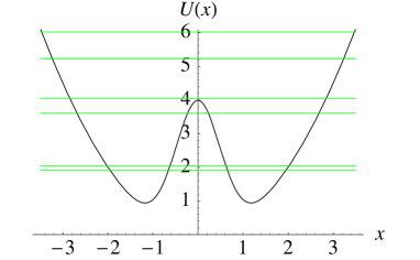
Figure 2: (color online) Single-particle spectrum $\left\{\epsilon_{a}\right\}$ in a double well with barrier height $h=5$.

The realistic single-particle spectrum is sketched in Fig. 2. Due to the nonzero width $w$, also the odd states are shifted slightly, and of course the distance between the doublets is never exactly $\Delta\epsilon=2$ as in the crude estimate above. What is more, the finite barrier $h=5$ not only lifts the even-odd degeneracy already for the lowest states, where the doublet character is still pronounced and the gap $\Delta_{h}\equiv\epsilon_{1}-\epsilon_{0}\ll 1$, but even more so for levels above the barrier. There the central region is classically allowed and the spectrum becomes more and more harmonic for higher $\epsilon_{a}$. The consequences for the full non-interacting spectrum $\sigma\left(H\right)$ in Fig. 3 are that the lowest band is ‘fanned up’ into $\{E_{m}=N\epsilon_{0}+m\Delta_{h}\}$. The next cluster of levels is still well separated in energy.

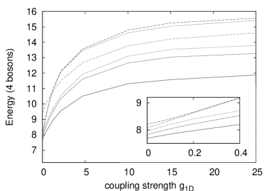
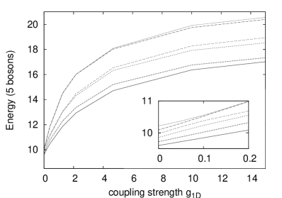
Figure 3: Lowest energies $E_{m}$ in a double well ($h=5$) for $N=3,4,5$ bosons. Inset ($N=4$): level adhesion for the states $m=3,4$ (counted from below at $g=0$).

The situation gets slightly more involved in the fermionization limit $g\to\infty$. Here the spectrum is generated by (fictitious) fermionic states $|\boldsymbol{n}\rangle$ with $n^{\prime}_{a}\in\{0,1\}$, so $E_{\boldsymbol{n}}=\sum_{a}n_{a}^{\prime}\epsilon_{a}$ is obtained by removing particles from below the Fermi edge $\epsilon_{N}=\mu_{N}$. The first excited state would thus be higher in energy by $\epsilon_{N}-\epsilon_{N-1}$, which—in our simplistic model invoked before—would be about zero for odd $N$ and two for even $N$. The next band would then be made up of four levels for any number of atoms, created by pushing one particle out of the doublet pertaining to $\epsilon_{N-1}$ into the next upper doublet. However, since these involve higher energies, the typical doublet structure encountered in the lowest levels is lost for our finite barrier $h=5$, and the spectrum will be rearranged and mixed, as seen in Fig. 3. Here the bands are no longer separated but smeared out considerably. Still, the odd-vs-even distinction with respect to the lowest level may be observed.

How do these two ends of the spectrum connect? As can be seen in Fig. 3, the reordering that is necessitated by the Bose-Fermi map starts taking place already for small $g$, where the influence of the interaction operator $H_{\mathrm{I}}:=\sum_{i<j}V(x_{i}-x_{j})$ can still be treated as a perturbation,

$$\Delta E_{\boldsymbol{n}}(g)\sim\langle H_{\mathrm{I}}\rangle_{\boldsymbol{n}}+\sum_{\boldsymbol{n}^{\prime}\neq\boldsymbol{n}}\frac{\left|\langle\boldsymbol{n}^{\prime}|H_{\mathrm{I}}|\boldsymbol{n}\rangle\right|^{2}}{E_{\boldsymbol{n}}(0)-E_{\boldsymbol{n}^{\prime}}(0)}.$$

In light of this, the different effects of $H_{\mathrm{I}}$ on different (non-interacting) states $|\boldsymbol{n}\rangle$ will manifest themselves in (i) their slopes and (ii) different curvatures. While the slopes $E^{\prime}(0)>0$ do not differ dramatically, the second order fosters level repulsion within each band, since the energy gaps are small in magnitude ($\left|E_{\boldsymbol{n}}(0)-E_{\boldsymbol{n}^{\prime}}(0)\right|=O(\Delta_{h=5})\ll 1$) but have different signs. (Needless to say, by conservation of parity $\Pi\Psi(Q)\equiv\Psi(-Q)$ solely states within the same symmetry subspace $\{\Psi\mid\Pi\Psi=\pm\Psi\}$ are coupled.) Even though limited to perturbative values $g<1$, this may help us understand why the upper lines of the lowest band tend to rise so steeply, whereas the lowest ones in each band are ‘pushed’ downward a little. For example, see Fig. 3, $N=4$: the two levels $m=3,4$ (counted at $g=0$) intersect the lowest upper-band state $|3,0,1\rangle$ at $g\simeq 1$.

Most stunning is the observation that, apparently, some lines are virtually ‘glued together’ once the interaction is switched on (see Fig. 3; insets $N=4,5$). In particular, this applies to the upper pair $m=N-1,N$ (counted at $g=0$, as always). To be sure, the two levels are close from the start ($\Delta E=\Delta_{5}\simeq 0.1$); but for $g\sim 1$ they get as close as $\sim 0.01$. This quasi-degeneracy arises as interactions are turned on; but it is destroyed again once these get very strong ($g\sim 5$). However, there is no indication as to what exact mechanism brings the two lines together. Not only do the corresponding states remain orthogonal at all couplings, but they stem from opposite-parity subspaces and can thus only mix with other states of a kind. Still, their reduced densities will turn out very much alike (as will be laid out in Sec. IV.2).

IV.2 Excited states

As yet, we have looked into the spectrum and its evolution from the weakly to the strongly interacting regime. In Sec. IV.1, we have found characteristic spectral patterns for the cases of a single and a double well, respectively. We now aspire to get a deeper insight into the underlying states $\Psi_{m\geq 1}$, which may be also beneficial for studying the dynamics in future applications.

Generally speaking, the non-interacting limit is described in terms of number states $|\boldsymbol{n}\rangle$ in the respective one-particle basis. Owing to the asymptotically harmonic confinement, we thus have an overall Gaussian profile $\rho(x)\propto\exp\left(-x^{2}\right)$, which is modulated by the central barrier as well as the degree of excitation. At least for the low-lying states, the length scale is therefore about that of the harmonic confinement, $a_{\parallel}=1$. Being single-particle states, they are essentially devoid of two-body correlations, which amount to $\rho_{2}=\frac{1}{2}(1+P_{12})\rho_{1}\otimes\rho_{1}$ (with the permutation operator $P_{12}$).

When interactions are added, some extra interaction energy $\frac{N(N-1)}{2}\mathrm{tr}\left(V\rho_{2}\right)$ must be paid. Hence, the system will respond by depleting the correlation diagonal $\rho_{2}(x_{1},x_{2}=x_{1}$), roughly speaking. In our single-particle expansion, this will be done by both adapting the single-particle functions $\varphi_{j}$ as well as by mixing different configurations $\Phi_{J}$ or—in the symmetrized version—$|\boldsymbol{n}\rangle$, depending on how close in energy they are. As $g\to\infty$, this culminates in the system’s fermionization, where there is a one-to-one correspondence to fermionic states, $n^{\prime}_{a}=0,1$. In particular, the density profile $\rho=\sum_{a}\left|\phi_{a}\right|^{2}$ becomes broader, with a length scale of order $\sqrt{2N}$ kolomeisky00 , while the strongly correlated nature is captured in the fermionic two-body density $\rho_{2}(x_{1},x_{2})=\left(\rho(x_{1})\rho(x_{2})-\left|\rho_{1}(x_{1},x_{2})\right|^{2}\right)/2$, which naturally vanishes at points of collision.

Harmonic trap ($h=0$)

Figure 4: Density profiles of $N=4$ bosons in a harmonic trap ($h=0$) for the excited states $m=1,2,3$ (from top to bottom).

Here the nature of the fermionization transition has been explored extensively for the ground state deuretzbacher06 ; zoellner06a ; zoellner06b . As for the excited states, a look at Fig. 4 unveils that essentially the same mechanisms are at work, as exemplified on the one-body density $\rho(x)$ for different states $m$. The non-interacting density profiles have a Gaussian envelope. This may be seen in the plot for $g=0.2$, the characteristic shape for the degenerate states $m=2,3$ stemming from the fact that the interaction $H_{\mathrm{I}}$ selects a linear combination so as to be diagonal within that subspace. Upon increasing $g$, the density is being flattened, reflecting the atoms’ repelling one another. Eventually, a fermionized state is reached, featuring characteristic humps in the density. As in the ground-state case, these signify localization; in other words, it is more likely to find one atom at discrete spots $x_{i}$. However, here the fermionization pattern eludes an obvious interpretation, since these are excited states. In particular, now the number of humps need not equal $N$, as can be seen for $m=1$.

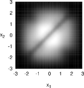
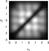
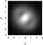
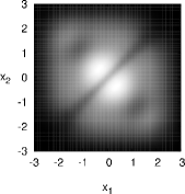
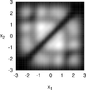
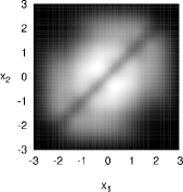
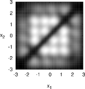
Figure 5: Two-particle density $\rho_{2}(x_{1},x_{2})$ for $N=4$ bosons in a harmonic trap. Top row: excited state $m=1,\dots$, bottom row: $m=3$; shown are the interaction strengths $g=0.2,\,2.2,\,15$ from left to right.

A look behind the scene is offered by the two-body correlation function $\rho_{2}$ (Fig. 5), which includes $\rho=\int dx_{2}\rho_{2}(\cdot,x_{2})$ by averaging over the second atom. It illustrates nicely how the interaction imprints a correlation hole at $\left\{x_{1}=x_{2}\right\}$, which relates to the washed-out profile in Fig. 4. A complex fragmentation of the $(x_{1},x_{2})$ plane can be witnessed as we go to larger $g$, which is different from the very obvious checkerboard pattern of the ground-state case zoellner06a . The latter one provided a simple interpretation, namely that the atoms are evenly distributed at discrete positions over the trap (up to a Gaussian density modulation), but with zero probability of finding two atoms at the same spot. Here the atoms are apparently more localized in the center. On top of that, if one atoms is fixed at some $x_{1}$, one cannot unconditionally ascribe definite positions for the $N-1$ remaining particles as before.

Double well ($h=5$)

Figure 6: Density profiles of $N=4$ bosons in a double well ($h=5$) for the lowest excited states $m=1,\dots,4$ (from top to bottom).

For large but finite barrier heights, the lowest excitations at $g=0$ will be formed by the two-mode vectors $|n^{\prime}_{0},N-n^{\prime}_{0}\rangle$. All of these will exhibit similar density profiles since $\rho(x)$ only differs significantly near the trap’s center; specifically $\rho(0)=n_{0}\left|\phi_{0}(0)\right|^{2}$. This can be seen in Fig. 6, which summarizes the evolution of the lowest excited states’ densities for $N=4$. As the perturbation $H_{\mathrm{I}}$ is turned on, different neighboring states $|\boldsymbol{n}\rangle$ (of equal symmetry) will be admixed, and the profiles are adjusted accordingly. Eventually, they saturate in the fermionic limit, featuring a typically broadened shape. Note that, for intermediate interactions (e.g., $g=1.3$), the aforementioned quasi-degenerate states $m=3,4$ (cf. Fig. 3) indeed reveal an almost identical profile.

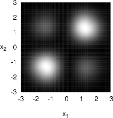
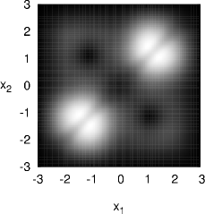
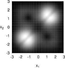
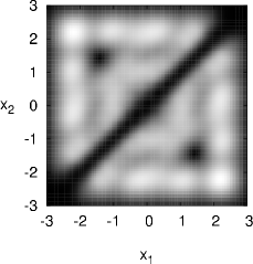
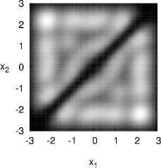
Figure 7: Two-particle density $\rho_{2}(x_{1},x_{2})$ for $N=4$ bosons in a double-well trap $(h=5)$. Left: excited state $m=3$, right: $m=4$; shown are the interaction strengths $g=0.2,\,1.3,\,25$ from top to bottom. The densities for both states are practically indistinguishable for mediate $g\sim 1$.

The same goes for the two-body density displayed in Fig. 7 for these two states ($m=3,4$). Absent any interactions, $\Psi_{4}$ stands out as it has pronounced off-diagonal peaks $\rho_{2}(x,-x)=\rho_{2}(x,x)=\left|\phi_{1}(x)\right|^{4}$, in contrast to $\Psi_{3}$. Already for small $g$, these are washed out due to admixing of neighboring states. For intermediate couplings, $g=1.3$, both densities become virtually indistinguishable. Eventually, also here the fermionization limit is reached, and the densities can be discriminated again. That said, it should once more be stressed that the respective states are by no means similar. Rather, they are described roughly through the orthogonal subspaces spanned by $\{|3,1\rangle,|1,3\rangle\}$ ($m=3$) and $\{|2,2\rangle,|0,4\rangle\}$ ($m=4$). Figure 8 sheds light on this aspect by laying out the evolution of the natural populations $n_{a}(g)$. It is similar for $m=3,4$ but not identical. The residual weights $n_{a\geq 2}$ are slightly separated from the dominant ones ($a=0,1$). However, as evidenced for the ground state zoellner06b , they cannot be neglected because they accumulate densely on a logarithmic scale, mirroring the extreme one-particle correlations imprinted in the course of fermionization.

Figure 8: Natural populations $n_{a}(g)$ ($a=0,\dots,3$ from top) for the excited states $m=3$ (—) and $m=4$ ($\cdots\cdots$) of $N=4$ bosons in a double well with barrier height $h=5$. Both are practically equal in energy and densities for mediate $g$.

IV.3 Crossover from single to double well

We have come a long way studying in depth the spectral properties of a single and a double well. As opposed to the ground-state case zoellner06a , the link between the two is far from obvious. In the harmonic trap, the fermionization transition was fairly tame, while in the presence of a fixed barrier $h=5$, there not only seemed to be a strikingly different level structure to begin with, but also the onset of a zoo of crossings and quasi-degeneracies. On that score, it would be desirable to get an understanding of the crossover from a single to a double well. To this end, we will again borrow some inspiration from the simple model of a point-split trap $h\delta(x)$ Busch03 .

Figure 9: Evolution of the natural orbitals $\phi_{a}$ as $h\to\infty$ for the case $N=3$ ($g=0.2$). Top: The first symmetric orbital $\phi_{0}$ is notched at $x=0$. Bottom: The antisymmetric one ($\phi_{1}$) is barely altered.

First consider the borderline case $g=0$. Then the one-particle occupations $\boldsymbol{n}$ are conserved for any parameter $h$, so we can assume number states $|\boldsymbol{n}\rangle$ as eigenstates (glossing over the fact that, of course, in the instance of degeneracy, the interaction operator will pick out a unitarily transformed basis diagonal in $H_{\mathrm{I}}$). Let us start with the harmonic trap ($h=0$), where the spectrum is arranged in steps of $\Delta_{0}=1$ according to $E_{\boldsymbol{n}}=\sum_{a}n^{\prime}_{a}(a+{\scriptstyle\frac{1}{2}})$ and the particles are distributed over the oscillator orbitals $\phi_{a}$. Now let us switch on a central barrier $h>0$ peaked at $x=0$. Then each even orbital $a\in 2\mathbb{N}$ will be notched at $x=0$, until its density $\left|\phi_{a}\right|^{2}$ will equal that of the next, odd orbital $\phi_{a+1}$. Figure 9 gives an illustration of this by displaying the natural orbitals $\phi_{0/1}$. Along that line, the energies will evolve continuously from $\epsilon_{a}$ to $\epsilon_{a+1}=a+{\scriptstyle\frac{3}{2}}$. On the other hand, granted that the barrier is supported exclusively at $x=0$, the odd orbitals themselves will remain completely untouched. Hence, in the limit $h\to\infty$, we would end up with a doubly degenerate single-particle spectrum (or, more realistically, a level gap $\Delta_{h}\ll 1$), which readily translates to a shift of $\Delta E_{\boldsymbol{n}}=\sum_{a\in 2\mathbb{N}}n^{\prime}_{a}\times 1=:n^{\prime}_{\mathrm{even}}$, depending on how many even orbitals were populated to begin with. Altogether, as the barrier $h$ is run up, the spectrum $\{N/2,N/2+1,\dots\}$ at $h=0$ is expected to transform into one with a lowest cluster of $1+N$ (quasi-)degenerate levels pertaining to $\{|n^{\prime}_{0},N-n^{\prime}_{0}\rangle\}$ at energies $E\sim 3N/2$, followed by another one at $E\sim 3N/2+2$.

It goes without saying that a realistic reasoning should take into account the finite barrier width ($w=0.5$), but the above toy model provides us with a rough picture to understand the crossover computed for $g=0.2$ in Fig. 10(a). Note that the sketched metamorphosis inevitably brings about crossings between different levels as $h\to\infty$ since, for instance, $|0,N\rangle$ is barely altered while $|n^{\prime}_{0},0,N-n^{\prime}_{0}\rangle$ is shifted by about $\Delta E\sim N$.

The above approach may be readily extended to the fermionization limit. All we need to do is construct auxiliary fermion states $\{|\boldsymbol{n}\rangle\mid n^{\prime}_{a}=0,1\}$ and apply the same machinery. However, a look at Fig. 10(b) ($g=15$) makes clear that the rearrangement of the levels is not as wild as as in the non-interacting case. That is simply because the ‘fermions’ can only occupy a level once; hence at $h\to\infty$ the lowest group is made up of one or two states only (for even/odd numbers, respectively), followed by a cluster of four levels regardless of the atom number. You might notice that the second band emerging as $h\to\infty$ is not perfectly bunched at $E(h=10)\simeq 11$, but really has a runaway at $E(h=10)\simeq 10.7$. This can be traced back to the inclusion of a higher orbital $\phi_{4}$ in the fermionic state: in such higher regions, the spectrum ceases to be perfectly doublet-like, foiling our previous considerations.

Figure 10: Crossover of the lowest energies $E_{m}(h)$ with varying barrier strength $h$ for $N=3$ bosons at interaction strengths $g=0.2$ (a); $g=15$ (b). The line styles are assigned so as to distinguish the different level groups at $h=0$.

For intermediate values of $g$, in turn, one cannot use the same line of argument since the interaction is in the way of a simple single-particle description, and $\boldsymbol{n}$ are no longer good quantum numbers. Still, the knowledge of the limiting cases highlighted above gives a guideline for the crossover. Generally speaking, changing $h$ for any $g$ will affect the energy via

$$\frac{d}{dh}E=N\mathrm{tr}\left(\rho_{1}\delta_{w}(x)\right)=N\bar{\rho}(0),$$

i.e, the coarse-grained density $\bar{\rho}\equiv\rho*\delta_{w}$ about the center will be reduced so as to minimize the energy costs. This will determine the fate of each state when changing over from a single to a double well, thus completing our picture of the lowest excitations in double-well traps.

V Conclusions and outlook

We have examined the lowest excitations of $N\leq 5$ bosons in harmonic and double-well traps, based on the numerically exact Multi-Configuration Time-Dependent Hartree method. The key aspect has been the spectral evolution from the weakly to the strongly interacting limit, this way extending our previous analyses of the ground state zoellner06a ; zoellner06b to the lowest excitations. Moreover, we have illuminated the crossover from a single well to a pronounced double well.

In the case of a purely harmonic trap, the initially equidistant and degenerate level structure is lifted as interactions are introduced, which distinguish between different states of the relative motion. In the fermionization limit of ultrastrong repulsion, a harmonic spectrum is recovered asymptotically. In a double well, the non-interacting spectrum has a lowest band composed of $N+1$ states formed from the (anti-)symmetric single-particle orbital, well separated from the next upper band. Here, the effect of interactions consists in a complex rearrangement of the levels, dominated by level repulsion in the perturbative regime. Moreover, some lines virtually adhere to one another as interactions are switched on, despite their being very different in character. In the fermionization limit, we end up with a lowest group made up of the ground state (even atom numbers) plus the first excited state (odd), followed by a cluster of four levels for any $N$, that washed out due to the non-doublet nature of the higher-lying orbitals.

In order to get a better understanding, we have also analyzed the underlying eigenvectors $\Psi_{m}$. At bottom, the same mechanism responsible for the ground-state fermionization could be identified. Stronger interactions imprint a two-body correlation hole, signifying a reduced probability of finding two particles at the same position, and eventually lead to localization. This becomes visible in the density profiles, which evolve from a Gaussian envelope to a significantly flatter shape. However, the excited states elude an intuitive interpretation applicable to the ground state.

Finally, we have cast a light on just how the spectrum is reorganized when splitting the purely harmonic trap into two fragments. To this end, we considered the deformation of the single-particle orbitals as a central barrier is run up. This leads to very different energy shifts depending on the overall population of even orbitals or, generally, the average density about the trap’s center.

With these systematic investigations, we have complemented the extensive work on the ground state. Numerically delicate as it is, our study has been limited to the lowest excitations and also to at most five atoms with an eye toward computing time. On the other hand, we hope it will also contribute to the understanding of dynamical but also thermal properties. In this light, an obvious extension would be to study time-dependent phenomena. Here double-well systems have proven to be a fruitful model for various phenomena.

- (1) L. Pitaevskii and S. Stringari, Bose-Einstein Condensation (Oxford University Press, Oxford, 2003).
- (2) F. Dalfovo, S. Giorgini, L. Pitaevskii, and S. Stringari, Rev. Mod. Phys. 71, 463 (1999).
- (3) C. J. Pethick and H. Smith, Bose-Einstein condensation in dilute gases (Cambridge University Press, Cambridge, 2001).
- (4) A. J. Leggett, Rev. Mod. Phys. 73, 307 (2001).
- (5) M. Olshanii, Phys. Rev. Lett. 81, 938 (1998).
- (6) M. Girardeau, J. Math. Phys. 1, 516 (1960).
- (7) H. G. Vaidya and C. A. Tracy, Phys. Rev. Lett. 42, 3 (1979).
- (8) A. Minguzzi, P. Vignolo, and M. P. Tosi, Phys. Lett. A 294, 222 (2002).
- (9) M. Girardeau, E. M. Wright, and J. M. Triscari, Phys. Rev. A 63, 033601 (2001).
- (10) T. Papenbrock, Phys. Rev. A 67, 041601 (2003).
- (11) T. Kinoshita, T. Wenger, and D. S. Weiss, Science 305, 1125 (2004).
- (12) B. Paredes et al., Nature 429, 277 (2004).
- (13) D. S. Petrov, G. V. Shlyapnikov, and J. T. M. Walraven, Phys. Rev. Lett. 85, 3745 (2000).
- (14) E. H. Lieb, R. Seiringer, and J. Yngvason, Phys. Rev. Lett. 91, 150401 (2003).
- (15) K. Sakmann, A. I. Streltsov, O. E. Alon, and L. S. Cederbaum, Phys. Rev. A 72, 033613 (2005).
- (16) Y. Hao, Y. Zhang, J. Q. Liang, and S. Chen, Phys. Rev. A 73, 063617 (2006).
- (17) T. Busch, B. G. Englert, K. Rzazewski, and M. Wilkens, Found. Phys. 28, 549 (1998).
- (18) D. Blume, Phys. Rev. A 66, 053613 (2002).
- (19) O. E. Alon and L. S. Cederbaum, Phys. Rev. Lett. 95, 140402 (2005).
- (20) F. Deuretzbacher, K. Bongs, K. Sengstock, and D. Pfannkuche, cond-mat/0604673 (2006).
- (21) A. I. Streltsov, O. E. Alon, and L. S. Cederbaum, Phys. Rev. A 73, 063626 (2006).
- (22) S. Zöllner, H.-D. Meyer, and P. Schmelcher, Phys. Rev. A 74, 053612 (2006).
- (23) S. Zöllner, H.-D. Meyer, and P. Schmelcher, Phys. Rev. A 74, 063611 (2006).
- (24) D. Masiello, S. B. McKagan, and W. P. Reinhardt, Phys. Rev. A 72, 063624 (2005).
- (25) D. J. Masiello and W. P. Reinhardt, cond-mat/0610609 (2006).
- (26) L. S. Cederbaum and A. I. Streltsov, Phys. Rev. A 70, 023610 (2004).
- (27) M. R. Andrews et al., Science 275, 637 (1997).
- (28) Y. Shin et al., Phys. Rev. Lett. 92, 050405 (2004).
- (29) T. Anker et al., Phys. Rev. Lett. 94, 020403 (2005).
- (30) H.-D. Meyer and G. A. Worth, Theor. Chem. Acc. 109, 251 (2003).
- (31) H.-D. Meyer, in The Encyclopedia of Computational Chemistry, edited by P. v. R. Schleyer et al. (John Wiley and Sons, Chichester, 1998), Vol. 5, pp. 3011–3018.
- (32) M. H. Beck, A. Jäckle, G. A. Worth, and H.-D. Meyer, Phys. Rep. 324, 1 (2000).
- (33) V. I. Yukalov and M. D. Girardeau, cond-mat/0507409 (2005).
- (34) G. A. Worth, M. H. Beck, A. Jäckle, and H.-D. Meyer, The MCTDH Package, Version 8.2, (2000). H.-D. Meyer, Version 8.3 (2002). See http://www.pci.uni-heidelberg.de/tc/usr/mctdh/.
- (35) R. Kosloff and H. Tal-Ezer, Chem. Phys. Lett. 127, 223 (1986).
- (36) H.-D. Meyer, F. L. Quéré, C. Léonard, and F. Gatti, Chem. Phys. 329, 179 (2006).
- (37) T. Busch and G. Huyet, J. Phys. B 36, 2553 (2003).
- (38) E. B. Kolomeisky, T. J. Newman, J. P. Straley, and X. Qi, Phys. Rev. Lett. 85, 1146 (2000).