Interacting anyons in topological quantum liquids: The golden chain
Abstract
We discuss generalizations of quantum spin Hamiltonians using anyonic degrees of freedom. The simplest model for interacting anyons energetically favors neighboring anyons to fuse into the trivial (‘identity’) channel, similar to the quantum Heisenberg model favoring neighboring spins to form spin singlets. Numerical simulations of a chain of Fibonacci anyons show that the model is critical with a dynamical critical exponent , and described by a two-dimensional (2D) conformal field theory with central charge . An exact mapping of the anyonic chain onto the 2D tricritical Ising model is given using the restricted-solid-on-solid (RSOS) representation of the Temperley-Lieb algebra. The gaplessness of the chain is shown to have topological origin.
pacs:
05.30.Pr, 73.43.Lp, 03.65.VfIntroduction
Non-Abelian anyons are exotic particles expected to exist in certain fractional quantum Hall (FQH) states MooreRead ; ReadRezayi . A set of several anyons supports very robust collective states that are degenerate to exponential precision; such states can potentially be used as quantum memory and for quantum computation ToricCode . However, this degeneracy can be lifted by a short-range interaction if the anyons are very close to each other. As a first step towards understanding interacting anyons, we describe a simple, exactly solvable model that is an anyonic analogue of the quantum Heisenberg chain.
We start by considering the well-known Moore-Read state MooreRead , a candidate state, exhibiting non-Abelian statistics, for the topological nature of FQH liquids at filling fraction . It has two important types of excitations: quasiholes with electric charge and neutral fermions. Quasiholes may be trapped by an impurity potential while the fermions can still tunnel between them ReadLudwig . For a one-dimensional (1D) array of trapped quasiholes, the Hamiltonian can be described in terms of free Majorana fermions on a lattice, which is in turn equivalent to the 1D transverse field Ising model at the quantum phase transition point. The more interesting model discussed here is based on so-called ‘Fibonacci anyons’, which represent the non-Abelian part of the quasiparticle statistics in the , -parafermion state ReadRezayi , an effective theory for FQH liquids at filling fraction TwelveFifth . Even without parameter fine-tuning, these 1D anyonic arrays will be shown to exhibit gapless excitations due to topological symmetry.
Model
Our model describes pairwise interactions within an array of anyons, for instance along a chain as shown in Fig. 1a). In the Fibonacci theory there are only two types of particles: the Fibonacci anyon, denoted by , and the trivial particle denoted by 1 with a fusion rule . We refer to the label or as the topological charge. When two neighboring anyons interact, indicated in the figure by the ellipses, they can either fuse in the trivial channel, annihilating each other, or in the nontrivial one, becoming a single -anyon Preskill . We define our model by assigning an energy gain if they fuse along the trivial channel. This is an anyonic analogue of the spin-1/2 quantum Heisenberg antiferromagnet, which assigns an energy gain to two neighboring spin-1/2 fusing into a spin-0 singlet as compared to a spin-1 triplet.
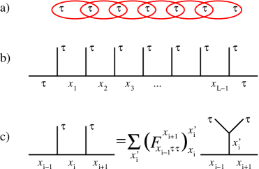
To define the Hilbert space of -anyons we consider the tree-like fusion diagram in Fig. 1b). The basis corresponds to all admissible labelings of the links, with or . Each label represents the combined topological charge of the particles left to a given point. Not all possible values represent allowed basis states due to the fusion rules: a must always be preceded and followed by a , since the fusion of a and a always gives a . This reduces the dimension of the Hilbert space of the open chain (with -labels at the boundary) to the Fibonnacci sequence dim, and for the periodic chain dim. For large it is well-known that these numbers grow at a rate , where is the golden ratio. This Hilbert space has no natural decomposition in the form of a tensor product of single-site states, in contrast to quantum spin chains.
In order to generate a local Hamiltonian assigning an energy to the fusion of two neighboring -anyons we use the so-called -matrix to transform the local basis as shown in Fig. 1c). In the transformed basis the state corresponds to the fusion of the two anyons. The Hamiltonian is then defined by assigning an energy for , and for . The resulting local terms contain three-body interactions in the link basis,
| (1) | |||
It is diagonal in the subspace , , where the -matrix is a number due to the constraints arising from the fusion rules. For the case , the -matrix and the corresponding Hamiltonian are the following -matrices ( )
| (2) |
Looking at the matrix form of the Hamiltonian, it can be written in terms of standard Pauli matrices:
where the sum runs over the links of the chain. In this expression, the operators count the -particle occupation on link , , and the Hamiltonian acts on the constrained Hilbert space defined above.
Entropy scaling and central charge
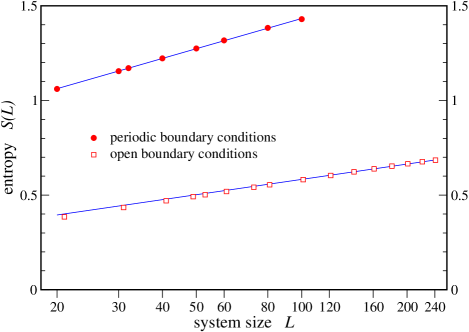
We simulated this model numerically, and calculated the finite-size excitation gap by exact diagonalization for chains of up to sites. A finite-size analysis shows that the gap vanishes linearly in , indicative of a critical model with dynamical critical exponent described by a conformal field theory. The central charge of a CFT can be calculated from the finite-size scaling of the entanglement entropy. For two subsystems with equal size on systems with periodic (PBC) and open boundary conditions (OBC) the entanglement entropy scales as entanglement
| (3) |
The density matrix renormalization group method (DMRG) DMRG ; DMRGdetails provides a natural framework for calculating these quantities. Fits of our numerical results according to Eqs. (3) shown in Fig. 2, give central charge estimates of and respectively. Since possible (unitary) CFTs in the vicinity of these estimates have central chargesFriedanQuiShenker , or we can unambiguously conclude that our results are consistent only with central charge .
Mapping and exact solution
We now proceed to derive these results exactly. By construction the local contribution to the Hamiltonian is a projector onto the trivial particle. One can then verify that the operators form a representation of the Temperley-Lieb algebra TemperleyLieb
| (4) |
where the ‘d-isotopy’ parameter equals the golden ratio, . This representation can be seen to be identical to the standard Temperley-Lieb algebra representation associated with at level . For arbitrary , the latter contains anyon species labelled by , satisfying the fusion rules of FusionRulesofSuTwoLevelK . The operators defined by
| (5) |
are known RefTemperleyLiebForSuTwoLevelK to form a representation of the Temperley-Lieb algebra (4) for any value of , where and FootnoteModularSmatrix .
Our model of interacting Fibonacci anyons can be cast into this form at by first mapping , and , and then applying the fusion rule to the even-numbered sites. This maps any admissible labeling uniquely into where for odd-numbered sites , and for even numbered-sites . This re-labeling maps the matrix elements of into those of from Eq. (5).
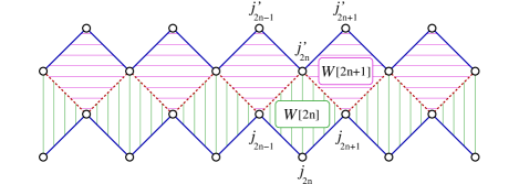
We can now see that the Hamiltonian in Eq. (1) is that corresponding to a standard (integrable) lattice model description of the classical 2D tricritical Ising model, known as the RSOS model RSOSmodel . Specifically, the two-row transfer matrix of this lattice model, shown in Fig. 3, is written in terms of Boltzmann weights assigned to a plaquette of the square lattice
with
| (6) |
The parameter is a measure of the lattice anisotropy, is the identity operator, and
| (7) |
The Hamiltonian of the so-defined lattice model is obtained from its transfer matrix by taking, as usual BaxterBook , the extremely anisotropic limit, ,
yielding ( is an unimportant constant). Since the operators can be identified with , this demonstrates that the Hamiltonian of the Fibonacci chain is exactly that of the corresponding RSOS model which is a lattice description of the tricritical Ising model at its critical point. The latter is a well-known (supersymmetric) CFT with central charge BPZ ; TricriticalIsingModel . Analogously one obtains Huse1984 for general the unitary minimal CFT FriedanQuiShenker of central charge . A ferromagnetically coupled Fibonacci chain (energetically favoring the fusion along the -channel) is described by the critical 3-state Potts model with and, for general , by the critical -parafermion CFT uReversedSign ; RSOSmodel ; Huse1984 with central charge .
Excitation spectra
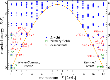
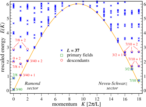
We have calculated the excitation spectra of chains up to size with open and periodic boundary conditions using exact diagonalization, as shown in Fig. 4. The numerical results not only confirm the CFT predictions but also reveal some important details about the correspondence between continuous fields and microscopic observables. In general, low-energy states on a ring are associated with local conformal fields CardyFSS1984 , whose holomorphic and antiholomorphic parts belong to representations of the Virasoro algebra, described by conformal weights and . The energy levels are given by
| (8) |
corresponding to states with a choice of momenta or in units of , where , are non-universal constants. Here, and , where correspond to weights of ‘primary’ fields and and are non-negative integers describing so-called ‘descendant’ fields. The numerical spectra for even values of (see the first plot in Fig. 4) agree with Eq. (8), exhibiting primary fields with , which are conventionally denoted by , respectivelyFootnoteOrderOperators . The momenta of the last two fields and their descendants are near , as compared to the other four, indicating that the corresponding microscopic observables have alternating sign on the lattice. Such “staggered” fields must have nontrivial monodromy with respect to a space-time dislocation (i.e., the insertion or removal of a site at some particular time). Such a dislocation is characterized by a chiral field, say, FermionicStressTensor . The of the monodromy factor matches the momenta in Fig. 4 FootnoteFusionEpsilon . Given this information, we may predict that the states of an odd size ring are associated with fields of the form , where . These include six primary fields, , , , , , , as well as their descendants. Integrality of the momentum dictates the choice of (see below Eq. (8)), as in Fig. 4.
| eigenvalue | numerics | CFT | numerics | CFT |
| assignment | assignment | |||
| 0 | 0.10 | 1/10 | 0 | 0 |
| 1 | 1.10 | 1/10 + 1 | 0.60 | 3/5 |
| 2 | 1.49 | 3/2 | 1.60 | 3/5 + 1 |
| 3 | 2.09 | 1/10 + 2 | 2.02 | 0 + 2 |
| 4 | 2.47 | 3/2 + 1 | 2.58 | 3/5 + 2 |
| 5 | 3.07 | 1/10 + 3 | 2.59 | 3/5 + 2 |
| 6 | 3.11 | 1/10 + 3 | 3.01 | 0 + 3 |
| 7 | 3.44 | 3/2 + 2 | 3.56 | 3/5 + 3 |
| 8 | 3.46 | 3/2 + 2 | 3.56 | 3/5 + 3 |
For open boundary conditions the spectra are known to be described by, say, the holomorphic sector only Boundary . To explain the numerical data, we need to assume that the ends of the chain are charaterized by a boundary field (or equally well ). Thus, for an even number of sites the spectrum is described by (plus descendants). For an odd number of sites, this result is to be modified by fusion with , yielding . The numerical low-energy spectra agree excellently with these predictions as shown in Table 1.
Hidden symmetries
The critical behavior of our model is not just a peculiarity of the exact solution but rather has topological origin. In general, an effective low-energy Lagrangian admits perturbations of the form , where may be any local field that is consistent with all applicable symmetries. Such terms are relevant if , in which case they may open a spectral gap or induce crossover to different critical behavior at large distances. In the tricritical Ising model, there are four relevant fields: , , , . Some explanation is in order as to why these fields do not appear in the effective Lagrangian of our model. The fields and are staggered and thus prohibited by translational symmetry. Excluding and requires a more subtle argument. The Fibonacci ring has a topological symmetry, which corresponds to adding an extra -line parallel to the spine of the fusion diagram (Fig. 1b) and merging it with the diagram using the -matrix. We denote this operator by .
where the identification is used. We may think of the fusion diagram as a description of a process that generates a set of -anyons on a circle from the local vacuum. Then describes another particle moving inside or outside that circle (or on the circle itself — before those anyons were created). The operator is sensitive to a possible topological charge located at the center of the circle. Thus has two eigenvalues, . We conjecture that the low-energy states associated with fields are in the the trivial () sector, and the fields are in the sector. In fact, the topological fusion algebra (defined by the rule ) is a quotient of the CFT fusion algebra.
We may imagine that the interaction between the anyons alters the topological liquid in which the anyons are excitations, producing an annulus of a different liquid. Some of the local fields correspond to the tunneling of a -anyon between the inner and outer edge of the annulus. Such a process is actually forbidden as it would change the topological charge . Thus, only fields in the trivial topological sector are allowed as perturbations. This excludes and .
Outlook
Extensions to chains of anyons in topological liquids described by Chern-Simons theory with corresponding (up to phases) to the non-abelian statistics of higher members of the Read-Rezayi series have been mentioned below Eq. (7), but their topological stability is an open issue. In analogy to quantum spin chains, additional interactions such as dimerization or coupling of two Fibonacci chains in a ladder geometry should lead to gapped quantum liquids. Disordered anyonic chains are currently being investigated Nick . For 2D anyonic structures gapless phases of non-Fermi liquid type might potentially also emerge.
We thank E. Ardonne, N. Bonesteel, P. Fendley, C. Nayak, G. Refael, S. H. Simon, and J. Slingerland for stimulating discussions. Some of our numerical simulations were based on the ALPS libraries ALPS .
References
- (1) G. Moore and N. Read, Nucl. Phys. B 360, 362 (1991).
- (2) N. Read and E. Rezayi, Phys. Rev. B59, 8084 (1999).
- (3) A. Yu Kitaev, Ann. Phys. 303, 3 (2003).
- (4) See e.g. N. Read and A.W.W. Ludwig, Phys. Rev. B 63, 024404 (2001).
- (5) J. S. Xia et al., Phys. Rev. Lett. 93, 176809 (2004).
- (6) For a pedagogical introduction we refer to J. Preskill, Lecture notes on quantum computation; available online at http://www.theory.caltech.edu/preskill/ph229
- (7) C. Holzhey et al., Nucl. Phys. B 424, 44 (1994); P. Calabrese and J. Cardy, J. Stat. Mech. P06002 (2004).
- (8) S. R. White, Phys. Rev. Lett. 69, 2863 (1992); U. Schollwöck, Rev. Mod. Phys. 77, 259 (2005).
- (9) The DMRG calculations were done for system sizes up to , keeping up to states. The constrained Hilbert space was implemented by explicitly adding a nearest-neighbor repulsion with .
- (10) N. Temperley and E. Lieb, Proc. Roy. Soc. Lond. A 322, 251 (1971).
- (11) D. Gepner and E. Witten, Nucl. Phys. B 278, 493 (1986); A. B. Zamolodchikov and V. A. Fateev, Sov. J. Nucl. Phys. 43, 657 (1986).
- (12) V. Jones, C. R. Acad. Sci. Paris Sér. I Math. 298, 505 (1984); A. Kuniba, Y. Akutsu, and M. Wadati, J. Phys. Soc. Jpn. 55, 3285 (1986); V. Pasquier, Nucl. Phys. B 285, 162 (1987); H. Wenzl, Invent. Math. 92, 349 (1988). For a recent discussion see: P. Fendley, J. Phys. A 39, 15445 (2006).
- (13) The matrix is the modular S-matrix of CFT.
- (14) G. E. Andrews, R. J. Baxter, and P. J. Forrester, J. Stat. Phys. 35, 193 (1984).
- (15) See for example: R. J. Baxter, Exactly solved models in statistical mechanics, Academic Press, London (1982).
- (16) D. Friedan, Z. Qiu, and S. Shenker, Phys. Lett. B 151, 37 (1985).
- (17) A. A. Belavin, A. M. Polyakov, and A. B. Zamolodchikov, Nucl. Phys. B 241, 333 (1984).
- (18) D. A. Huse, Phys. Rev. B 30, 3908 (1984).
- (19) D. Friedan, Z. Qiu and S. Shenker, Phys. Rev. Lett. 52, 1575 (1985).
- (20) Here the sign of in Eq. (6) is reversed RSOSmodel as compared to the antiferromagnetic case.
- (21) J. L. Cardy, J. Phys. A 17, L385 (1984); Nucl. Phys. B 270, 186 (1986).
- (22) is the superpartner of the stress tensor in this superconformal theory TricriticalIsingModel .
- (23) We used the fact that the fusion with correponds the mapping: , , , . The complete set of fusion rules can be found in BPZ , see e.g. also: P. Di Francesco, P. Mathieu, and D. Sénéchal, Conformal Field Theory, Springer, New York (1997).
- (24) The last two fields are the order operators, i.e. those coupling to applied magnetic fields in the tricritical Ising model.
- (25) N. Bonesteel, private communication
- (26) J. L. Cardy, Nucl. Phys. B 240, 514 (1984).
- (27) F. Alet et al., J. Phys. Soc. Jpn. Suppl. 74, 30 (2005).