Topological defects and electronic properties in graphene.

In this work we will focus on the effects produced by topological disorder on the electronic properties of a graphene plane. The presence of this type of disorder induces curvature in the samples of this material, making quite difficult the application of standard techniques of many body quantum theory. Once we understand the nature of these defects, we can apply ideas belonging to quantum field theory in curved space-time and extract information on physical properties that can be measured experimentally.

1 Introduction

Graphene is a two dimensional material formed by isolated layers of carbon atoms arranged in a honeycomb-like lattice.

Each carbon atom is linked to three nearest neighbors due to the $sp^{2}$ hybridization process, which leads to three strong $\sigma$ bonds in a plane and a partially filled $\pi$ bond, perpendicular to the plane. These $\pi$ bonds will determine the low energy electronic and transport properties of the system.

It is possible to derive a long wavelength tight binding hamiltonian for the electrons in these $\pi$ bonds(Wallace (1947)). This hamiltonian is:

$$H=-iv_{F}\int d^{2}\textbf{r}\bar{\Psi}(\textbf{r})\gamma^{j}\partial_{j}\Psi(\textbf{r}),$$ (1)

where $v_{F}$ being a constant with dimensions of velocity ($v_{F}\sim 10^{3}m/s$). The wave equation derived from the hamiltonian (1) is the Dirac equation in two dimensions with the coefficients $\gamma^{j}$ being an appropriate set of Dirac matrices. We can set for instance, $\gamma^{1}=\mathbf{1}\otimes\sigma_{1}$ and $\gamma^{2}=\tau_{3}\otimes\sigma_{2}$, where the $\sigma,\tau$ matrices are related to the sublattice and Fermi point degrees of freedom respectively. The unexpected form of the tight-binding Hamiltonian comes from two special features of the honeycomb lattice: first, the unit cell contains two carbon atoms belonging to different triangular sublattices, and second, in the neutral system at half filling, the Fermi surface reduces to two nonequivalent Fermi points. We will study the low energy states around any of these two Fermi points. The dispersion relation obtained from (1) is $\varepsilon(\textbf{k})=\pm v_{F}|\textbf{k}|$, leading to a constant density of states, $\rho^{0}(\omega)=\frac{8}{\pi}|\omega|$.

2 A first model for the topological defects in graphene

Several types of defects like vacancies, adatoms, complex boundaries, and structural or topological defects have been observed experimentally in the graphene lattice(Hashimoto et al. (2004)) and studied theoretically (see for example Lehtinen et al. (2003),Vozmediano et al. (2005), López-Sancho et al. (2006)).
Topological defects are produced by substitution of an hexagonal ring of the honeycomb lattice by an n-sided polygon with any n. Their presence impose non-trivial boundary conditions on the electron wave functions which are difficult to handle. A proposal made in González et al. (1992) was to trade the boundary conditions imposed by pentagonal defects by the presence of appropriate gauge fields coupled to the spinor wave function. A generalization of this approach to include various topological defects was presented in Lammert and Crespi (2004). The strategy consists of determining the phase of the gauge field by parallel transporting the state in suitable form along a closed curve surrounding all the defects.

$$\Psi(\theta=0)=T_{C}\Psi(\theta=2\pi)\Leftrightarrow\Psi(\theta=0)=\exp({\oint_{{}_{C}}\textbf{A}_{a}T^{a}d\textbf{r}})\Psi(\theta=2\pi),$$ (2)

where $\textbf{A}_{a}$ are a set of gauge fields and $T^{a}$ a set of matrices related to the pseudospin degrees of freedom of the system.
When dealing with multiple defects, we must consider a curve surrounding all of them, as the one sketched in figure (1):

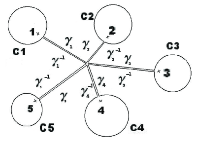
Figure 1: Scheme of a prototypical curve enclosing multiple defects in which the state will be parallel transported.

The contour C is made of closed circles enclosing each defect and straight paths linking all the contours to a fixed origin. The parallel transport operator $P_{C}$ associated to the closed path is thus a composition of transport operators over each piece:

$$P=P_{\gamma 1}\cdot P_{1}\cdot P^{-1}_{\gamma 1}\cdot...\cdot P_{\gamma N}\cdot P_{N}\cdot P^{-1}_{\gamma N}.$$ (3)

As explained in Lammert and Crespi (2004)the total holonomy turns out to be:

$$P=(i)^{N}(\tau_{2})^{N}exp\left(\frac{2\pi i}{6}(N^{+}-N^{-})\sigma_{3}\right)exp\left(\frac{2\pi i}{3}\sum^{N}_{j=1}(n_{j}-m_{j})\tau_{3}\right).$$ (4)

From equation (4) we see that we have in principle three different gauge fields to incorporate into the Dirac equation, which couple to the matrices $\sigma_{3}$, $\tau_{2}$, and $\tau_{3}$ and whose associated fluxes are adjusted from (2).

3 Generalization of the model

In spite of its elegance, the model presented in the previous section does not contain the effects due to the curvature of the layer in the presence of these defects. The model can be generalized to account for curvature effects (González et al. (1992), Kochetov and Osipov (1999)) by coupling the gauge theory obtained from the analysis of the holonomy in a curved space.

The substitution of a hexagon by a polygon with $n<6$ sides gives rise to a conical singularity with deficit angle $(2\pi/6)(6-n)$, which is similar to the singularity generated by a cosmic string in general relativity. The Dirac Equation for a massless spinor in a curved spacetime is (Birrell and Davis (1982)):

$$i\gamma^{\mu}(x)(\partial_{\mu}-\Gamma^{(T)}_{j\mu})\psi=0,$$ (5)

where $\Gamma^{(T)}_{j\mu}$ is a set of spin connections related to the pseudospin matrices in (4) and $\gamma^{\mu}(x)$ are generalized Dirac matrices satisfying the anticommutation relations

$$\left\{\gamma^{\mu}(x),\gamma^{\nu}(x)\right\}=2g^{\mu\nu}(x).$$ (6)

The metric tensor in (6) corresponds to a curved spacetime generated by an arbitrary number of $N$ parallel cosmic strings placed in $(a_{i},b_{i})$ (here we will follow the formalism developed in Aliev et al. (1997)):

$$ds^{2}=-dt^{2}+e^{-\Lambda(x,y)}(dx^{2}+dy^{2}),$$ (7)

with $\Lambda(x,y)=\sum^{N}_{i=1}4\mu_{i}\log([(x-a_{i})^{2}+(x-b_{i})^{2}]^{1/2})$. The parameters $\mu_{i}$ are related to the angle defect or surplus by the relationship $c_{i}=1-4\mu_{i}$ in such manner that if $c_{i}<1(>1)$ then $\mu_{i}>0(<0)$.
From equation (5) we can write down the equation for the electron propagator, $S_{F}(x,x^{\prime})$:

$$i\gamma^{\mu}(x)(\partial_{\mu}-\Gamma^{(T)}_{j\mu})S_{F}(x,x^{\prime})=\frac{1}{\sqrt{-g}}\delta^{3}(x-x^{\prime}).$$ (8)

The local density of states $N(\omega,\textbf{r})$ is obtained from the solution of (8) by Fourier transforming the time component and taking the limit $\textbf{r}^{\prime}\rightarrow\textbf{r}$:

$$N(\omega,\textbf{r})=ImTrS_{F}(\omega,\textbf{r},\textbf{r}).$$ (9)

Provided that we only consider the presence of pentagons and heptagons, the parameters $\mu_{i}$ are all equal and small ($\mu_{i}\equiv\mu=1/24$). We will solve equation (8) perturbatively in $\mu$.
When dealing with equation (8) we will reduce the number of spin connections derived in the previous section by the following considerations: First, we will consider an scenario where the number of pentagonal and heptagonal defects is the same - so the total number of defects is even. This suppresses the contribution from the first exponential in (4). If we consider that pentagonal and heptagonal defects come in pairs as usually happens in the observations, we can neglect the effect of mixing of the the two sublattices that each individual odd-sided ring produces and hence eliminate the spin connection related to $\tau_{2}$ from (8). Furthermore, we can disregard the spin connection related to $\tau_{3}$ by the following argument:

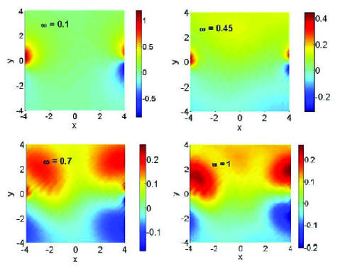
Figure 2: First order correction to the local density of states in a region around two pairs of heptagon-pentagon defects located out of the image for increasing values of the energy.

We will solve equation (8) perturbatively to first order of the parameter $\mu$. In general if $S^{0}_{F}$ is the unperturbed Dirac propagator and $\hat{V}(\omega,\textbf{r})$ the perturbation potential, the first term of such solutions is:

$$S^{1}_{F}(\omega,\textbf{r},\textbf{r}^{\prime})=\mu\int d^{2}\textbf{r}^{\prime\prime}S^{0}_{F}(\omega,\textbf{r},\textbf{r}^{\prime\prime})\hat{V}(\omega,\textbf{r}^{\prime\prime})S^{0}_{F}(\omega,\textbf{r}^{\prime\prime},\textbf{r}^{\prime}),$$ (10)

and we trace $S^{0}_{F}(\omega,\textbf{r},\textbf{r})$ in order to get the first contribution to the density of states $\delta N(\omega,\textbf{r})$. The trace operation eliminates all the terms appearing in (10) which are proportional to a traceless matrix, including the matrix related to $\tau_{2}$. In fact, up to this order in perturbation theory, the only term that survives will be the one proportional to $\gamma^{0}$. With all this in mind, the relevant spin connection terms are:

$$\Gamma_{1}(\textbf{r})=-\frac{1}{2}\gamma^{1}\gamma^{2}\partial_{y}\Lambda,\Gamma_{2}(\textbf{r})=-\frac{1}{2}\gamma^{2}\gamma^{1}\partial_{x}\Lambda.$$ (11)

After all these simplifications we can write equation (8) in a more suitable form. Expanding the terms in (11) in powers of $\mu$ we get the potential $\hat{V}(\omega,\textbf{r})$:

$$\hat{V}(\omega,\textbf{r})=-2\Lambda\gamma^{0}\omega+i\Lambda\gamma^{j}\partial_{j}+\frac{i}{2}\gamma^{j}(\partial_{j}\Lambda).$$ (12)

As we said, expression (10) gives us the first correction to the local density of states in real space. In figure (2) we present an example of the results obtained. We show the first order correction to the local density of states coming from two pairs of heptagon-pentagon defects located out of the image for increasing values of the energy. What we see is that as the frequency increases, the local density of states is enhanced and inhomogeneous oscillations are observed in a wide area around the defects. The spatial extent of the correction is such that the relative intensity decays to ten percent in approximately 20 unit cells. The model described in this work can be applied to other configurations of defects, such as simple pairs or stone-Wales defects. These results can be found in (Cortijo and Vozmediano (2006)).

Acknowledgements: Funding from MCyT (Spain) through grant FIS2005-05478-C02-01 and European Union FERROCARBON Contract 12881 (NEST) is acknowledged.

References

- Wallace (1947) P. R. Wallace, Phys. Rev. 71, 622 (1947).
- Hashimoto et al. (2004) A. Hashimoto, K. Suenaga, A. Gloter, K. Urita, and S. Iijima, Nature 430, 870 (2004).
- Lehtinen et al. (2003) P. O. Lehtinen, A. S. Foster, A. Ayuela, A. V. Krasheninnikov, K. Nordlund, and R. M. Nieminen, Phys. Rev. Lett. 91, 017202 (2003).
- Vozmediano et al. (2005) M. A. H. Vozmediano, M. P. López-Sancho, T. Stauber, and F. Guinea, Phys. Rev. B 72, 155121 (2005).
- López-Sancho et al. (2006) M. P. López-Sancho, T. Stauber, F. Guinea, and M. A. H. Vozmediano (2006), contribution in this volume.
- González et al. (1992) J. González, F. Guinea, and M. A. H. Vozmediano, Phys. Rev. Lett. 69, 172 (1992).
- Lammert and Crespi (2004) P. E. Lammert and V. H. Crespi, Phys. Rev. B. 69, 035406 (2004).
- Kochetov and Osipov (1999) E. A. Kochetov and V. A. Osipov, J. Phys. A 32, 1961 (1999).
- Birrell and Davis (1982) Birrell and Davis, Quantum fields in curved space (Cambridge University Press, 1982).
- Aliev et al. (1997) A. N. Aliev, M. HÖrtacsu, and N. Ozdemir, Class. Quantum. Grav. 14 (1997).
- Cortijo and Vozmediano (2006) A. Cortijo and M. A. H. Vozmediano (2006), cond-mat/0603717.