Two-level systems coupled to an oscillator: Excitation transfer and energy exchange

Abstract

We consider models in which two sets of matched two-level systems are coupled to a common oscillator in the case where the oscillator energy is small relative to the two-level transition energies. Since the two sets of two-level systems are coupled indirectly through the oscillator, excitation transfer from one set of two-level systems to the other is possible. In addition, the excitation energy from the two-level systems may be exchanged with the oscillator coherently, even though the oscillator energy may be orders of magnitude smaller than the two-level system transition energy. In the lossless case, we demonstrate these effects numerically, and also use an approximate diagonalization to show that these effects are expected from the model Hamiltonian.

We augment the model to include loss effects, and show that loss enhances the excitation transfer effect by breaking the severe cancelation between different paths that occurs in the lossless case. We describe a simple approximate model wavefunction appropriate when the loss increases rapidly with energy. Within this model approximation, we present numerical and analytical results for excitation transfer and energy transfer rates, showing that they are greatly increased.

Our study of these models is motivated in part by claims of excess heat production in electrochemical experiments in heavy water. We examine the question of whether the rates associated with this kind of model are sufficiently large to be relevant to the experimental claims. We find that consistency is possible given recent experimental results showing strong screening effects in low energy deuteron-deuteron fusion experiments in metals.

I Introduction

The Department of Energy conducted a review of cold fusion in 2004 that included excess heat experiments as the primary focus of the written review material and oral presentations.ReviewDoc Although the reviewers were not asked to respond on the specific issue of excess power (which has been the main goal of most of the experimental efforts), most of the reviewers volunteered comments on this aspect of the review material. A majority of these comments were favorable.reviewcomments In addition, most of the reviewers recommended that research in this area be funded, and there was strong encouragement that those working in the field should present their results in the mainstream scientific journals.

In successful experiments of this type, deuterium is introduced into a sample, the sample is stimulated, and a large amount of energy is observed as thermal output. There are essentially no energetic nuclear products (such as neutrons, gammas, alphas, betas, or x-rays that would signify the presence of energetic charged particles) seen in quantitative correlation with the energy. There is evidence for the production of helium in an amount quantitatively correlated with the excess energy, such that an energy of about 24 MeV is measured in association with each ⁴He atom detected. There is no evidence that this helium was created with any significant kinetic energy. A review of these issues and some discussion of the associated experiments is given in the document prepared for the 2004 DoE review.ReviewDoc

With this as motivation, we are interested here in possible physical mechanisms that may be involved, under the assumption that the excess heat effect is real. When two deuterons react in vacuum, the primary reaction channels are n+³He and p+t, with the reaction energy expressed as relative kinetic energy of the products, consistent with our notions of energy and momentum conservation. However, we know that the energy in these experiments is not due to the vacuum reaction pathway, since the vacuum reaction products are not present in quantitative amounts. We would also not expect that these reactions should be responsible for the energy observed, since from vacuum nuclear physics the associated reaction rates are quite small.

Whatever processes are responsible for the excess heat effect, they have not been seen before in nuclear physics or condensed matter physics. According to the 1989 DoE ERAB reportERAB : “Nuclear fusion at room temperature, of the type discussed in this report, would be contrary to all understanding gained of nuclear reactions in the last half century; it would require the invention of an entirely new nuclear process.” In this work, we consider models which correspond to proposed new physical processes.

I.1 Basic scheme

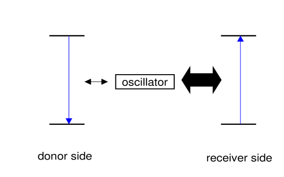
Figure 1: Schematic of two sets of two-level systems coupled to a common highly excited oscillator. The coupling between the donor side two-level systems and the oscillator is assumed to be weak, as indicated by a small arrow between them. The coupling between the receiver side two-level systems and oscillator is assumed to be strong, as indicated by a large arrow between them.

For the past several years we have been studying a new class of candidate reaction mechanisms to account for the excess heat effect. At the heart of these physical mechanisms is the basic scheme illustrated in Figure 1. In this figure, we show two sets of two-level systems which are individually coupled to a common oscillator. On the donor side, the upper level is associated with molecular D₂, and the lower level is associated with ⁴He. On the receiver side, the lower level is associated with a ground state receiver nucleus, such as a Pd isotope. The upper level is associated with a (reasonably stable) excited state in the receiver nucleus. Operation of the scheme involves the transfer of excitation from the two-level systems on the donor side to the two-level systems on the receiver side, and subsequent loss of excitation on the receiver side. The coupling on the donor side is assumed to be weak, since the two deuterons must tunnel through a Coulomb barrier in order to interact. The coupling on the receiver side is assumed to be strong, since there is no requirement for tunneling through a large barrier.

I.2 Excitation transfer and energy exchange effects

From the literature on the closely-related spin-Boson problem,Cibils1991 one would expect interesting (fast) oscillatory dynamics in this kind of model to occur near the oscillator frequency, and also near frequencies associated with the two-level transitions energies. Such effects are not of interest to us in this work. Instead, we are concerned with two different effects (excitation transfer and energy exchange) which occur on a slower timescale (in the absence of loss). The excitation transfer effect (as we use the term in this paper) involves moving excitation from one set of two-level systems to the other, through indirect coupling with the oscillator. The energy exchange effect (as we use the term in this paper) involves an increase (or decrease) of oscillator energy in association with a corresponding decrease (or increase) in the number of excited two-level systems. These effects are weak in the absence of loss, and it is only specially constructed solutions for models where resonance conditions are precisely matched that show these effects clearly. The possibility that energy can be exchanged coherently between two quantum systems with incommensurate energies is not widely appreciated, and one of the goals of this manuscript is to draw attention to it through models, analytic results, and numerical calculations. The analysis of this manuscript focuses on the coupling with a single highly-excited phonon mode (the oscillator in Figure 1), hence coupling to other modes is not a focus of the models. As a result, we do not obtain here an estimate for loss of two-level excitation through sequential incoherent phonon exchange.

Excitation transfer as a quantum effect is well known; in biophysics and nanoscale physics, one encounters Förster excitation transfer, in which Coulombic dipole coupling between molecules allows excitation at one location to be transferred to another location.Forster ; RET1999 There is no possibility of a Förster type of (Coulomb-mediated) excitation transfer between nuclei at the MeV energy scale analogous to the effect in atoms and molecules. Instead, we focus on a second-order indirect version of the effect. This kind of scheme has been considered previously in association with the possibility of indirect excitation transfer of optical excitation through coupling with a common microwave mode.XRL Here, excited nuclear states are assumed to couple to a common phonon mode, with a resulting indirect second-order coupling to excited nuclear states at other sites. Such indirect coupling has the potential to support a site-to-other-site excitation transfer effect. An indirect excitation transfer effect of this kind should in principle be possible when two atoms or molecules are coupled to a common phonon mode. However, we are not aware of this kind of indirect second-order process having yet produced an important contribution in an experiment. Second-order indirect coupling itself is discussed widely in the literature.Juzel1994 Indirect coupling between quantum well states interacting with a common phonon mode has been discussed in the literature.Vorrath2003

I.3 Overview of the paper

The number of issues involved in this scheme is very large, and we have no hope of addressing them all here. Instead, we focus attention on basic issues associated with the idealized model illustrated in Figure 1, to develop understanding of the excitation transfer and energy exchange mechanisms. The layout of the paper is as follows. We begin in Section II with a discussion of the basic model for two sets of two-level systems coupled to a common oscillator. We present numerical results which illustrate the presence of an excitation transfer effect and energy exchange effect. Since the idealized model is relatively simple, we are able to apply a rotation that brings out terms which exhibit these effects individually. Both effects in this model are quite weak, and require precise resonances to be observed.

In Section III, we augment the model to include loss. The specific loss mechanisms that are most relevant to the discussion are those in which a unit of two-level transition energy is lost. This can occur through the decay of excited states, or through more subtle processes in which the coupled system is capable of dissipating a large quantum of energy through a variety of decay modes. These latter processes have a big impact on the quantum states and associated dynamics, and are of much interest to us in this paper (we assume that the physical states associated with the two-level systems are reasonably stable at their given energies). Loss mechanisms are discussed in Appendix A. The impact of loss on excitation transfer is examined using perturbation theory. The associated indirect coupling in the lossless model is weak due to destructive interference between different pathways. This destructive interference is removed when loss is included, which leads to a dramatic increase in the indirect interaction.

In Section IV, we focus on energy exchange between the two-level systems on the receiver side and the oscillator in the presence of loss (at the two-level transition energy). To make quantitative estimates, we require a specification of the loss terms in the Hamiltonian. The inclusion of loss results in a dramatic increase in rates over the lossless case as mentioned above; however, different loss models produce only minor changes in the increased rates. In Appendix B we discuss an approximate wavefunction in which parts which see significant loss are omitted. Such an approximate wavefunction would result from a loss model in which the loss increases strongly with energy. The advantage of this kind of approximation is that it leads to a well-defined and simple approximate wavefunction which can be used to evaluate lossy models systematically, and that it brings out the dominant effects associated with the inclusion of loss in the model. We make use of this approximation in order to develop numerical results for energy exchange in the case of intermediate coupling, and analytic results (Appendix C) in the case of strong coupling. In Section V, we focus on excitation transfer between donor and receiver two-level systems. We again make use of the approximate wavefunction discussed in Appendix B for a direct numerical calculation of excitation transfer in the case of intermediate coupling, and analytic results (Appendix D) in the case of strong coupling.

In Section VI, we revisit the issue of excitation transfer using a different approach. In the limit that the number of oscillator quanta is very large and many two-level systems are involved, then we may model the system locally as being periodic. Calculations of the associated band structure leads to estimates of the group velocity associated with excitation transfer which compare well with the analytic results obtained in Appendix D. One new feature that results from this model is that we find that excitation transfer can proceed at nearly the maximum rate possible, even in the absence of a precise resonance when the receiver-side two-level systems are strongly coupled to the oscillator. This very interesting result can be understood as involving a coupling of energy directly with the oscillator to make up the power loss or gain associated with mismatched excitation transfer.

In Section VII, we consider the excitation transfer rate (assuming it is rate limiting) in comparison with excess power production in excess heat experiments. It is not possible to obtain consistency without the inclusion of screening effects. Experimental results indicate the presence of strong screening at low energies; however, a quantitative explanation for the effect from theory is currently lacking. In light of this situation, we conclude that the model results appear to be consistent with excess heat given what seems to be a reasonable value for the (zero-relative energy) screening energy.

In Section VII, we summarize our results and provide some discussion of the significance.

II Sets of two-level systems coupled to an oscillator

Our first goal is to present a highly idealized model which illustrates the excitation transfer and energy transfer effects. We study an idealized Hamiltonian that describes two sets of two-level systems coupled to an oscillator. Such a model exhibits both excitation transfer and energy transfer effects, as can be shown by a direct numerical solution. Because the Hamiltonian is relatively simple, we are able to develop an approximate diagonalization. The result of this approximate diagonalization is the development of an interaction term that corresponds to the excitation transfer effect discussed above, as well as an interaction term that can couple energy between the receiver-side two-level systems and the oscillator.

II.1 Idealized model

The associated Hamiltonian is

$$\hat{H}~{}=~{}\Delta E_{1}{\hat{S}_{z}^{(1)}\over\hbar}+\Delta E_{2}{\hat{S}_{z}^{(2)}\over\hbar}+\hbar\omega_{0}\hat{a}^{\dagger}\hat{a}+V_{1}e^{-G}{2\hat{S}_{x}^{(1)}\over\hbar}(\hat{a}+\hat{a}^{\dagger})+V_{2}{2\hat{S}_{x}^{(2)}\over\hbar}(\hat{a}+\hat{a}^{\dagger})$$ (1)

where the oscillator energy is presumed to be much less than the transition energy of the two-level systems

$$\hbar\omega_{0}\ll\Delta E_{1}\ \ \ \ \ \ \ \ \ \ \hbar\omega_{0}\ll\Delta E_{2}$$ (2)

We see in this model a set of two-level systems with transition energy $\Delta E_{1}$ which are weakly coupled to the oscillator. We use a pseudospin $\hat{S}_{z}$ operator to keep track of how many of the two-level systems are excited. Transitions from the upper state to the lower state are described using the pseudospin $\hat{S}_{x}$ operator, which assumes that the coupling is independent of which two-level system is involved, and that we would expect Dicke enhancement factorsDicke to be present. The strength of this coupling is $V_{1}e^{-G}$, where the presence of the Gamow factor $e^{-G}$ signals that this transition is hindered. We have assumed linear coupling with the oscillator for simplicity, although our basic results would change little had we instead used a weak nonlinearity. We see a second set of two-level systems with transition energy $\Delta E_{2}$ which are more strongly coupled to the oscillator. We assume that the oscillator is linear.

II.2 Numerical solution exhibiting excitation transfer effect

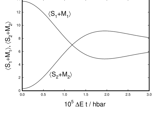
Figure 2: Demonstration of excitation transfer in the loss-free system. Expectation values of the number of excited two-level systems from a numerical calculation with one set of 14 two-level systems transferring excitation to a second set of 14 two-level systems. In this calculation, we used $V_{2}\sqrt{n_{0}}/\Delta E=0.1$. Since excitation transfer requires precise resonances, we chose $V_{1}e^{-G}\sqrt{n_{0}}/\Delta E=0.1$ in order to maximize the total amount of excitation transfer in this example. We used a window of oscillator quanta with $n_{0}\leq n\leq n_{0}+21$, where the oscillator energy is 0.03 $\Delta E$. A time-dependent wavefunction was constructed of the 15 nearly resonant eigenfunctions, and initialized to maximize the probability of occupation of the state with 14 excited two-level systems in the first set, no excited two-level systems in the second set, and 10 oscillator quanta.

We consider now two numerical solutions to the Schrödinger equation to illustrate the effects under discussion. We show first the excitation transfer effect, in which the excitation of two-level systems in the first system are transferred to the second-system. The result of a calculation is presented in Figure 2 which shows excitation transfer from one set of 14 two-levels systems to a second set of 14 two-level systems. Excitation transfer in this idealized model is a slow process that depends critically on the energies being resonant. Since coupling with the oscillator produces a self-energy shift, the most dramatic effect can be obtained under conditions where the two sets of two-level systems are matched in number and coupling strength. Consequently, we have chosen to illustrate this effect here with a matched system (even though we are interested in the model when the coupling on the donor side is hindered). In addition, the strongest indirect coupling effect is developed when the number of oscillator quanta is not so great, since the relative strength of indirect coupling in this model is reduced by $O(n)$ (due to severe cancelation of terms from different paths) as compared to the first-order interaction. The numerical calculation in this case illustrates that excitation transfer is present in this model, and that the associated rate is slow.

II.3 Numerical solution exhibiting energy exchange effect

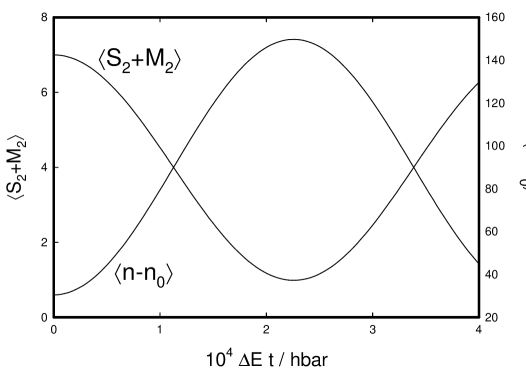
Figure 3: Demonstration of energy exchange in the loss-free system. Expectation values of the number of excited two-level systems from a numerical calculation with 8 receiver-side two-level systems coupled to an oscillator. For this calculation we used an oscillator energy of $\hbar\omega_{0}=\Delta E_{2}/11$, and a coupling strength of $V_{2}\sqrt{n_{0}}/\Delta E_{2}=0.33744$. This coupling strength is selected so that the dressed receiver-side transition energy approximately matches 15 oscillator quanta (since the dressed states are made up of a superposition of different $M_{2}$ states, the mixed states occur at roughly 0.76 $M_{2}$, so that roughly 20 oscillator quanta make up one bare two-level system quantum). For simplicity, we assumed no coupling with the first set of two-level systems. The total number of oscillator quanta in this calculation is chosen to be $10^{8}$. In this calculation, approximately resonant eigenfunctions were combined to make a time-dependent solution that is initialized with the receiver-side two-level systems nearly completely excited. One sees that the energy of the two-level systems is transferred slowly to the oscillator and back.

We next examine energy exchange on the receiver side. To illustrate this effect, we consider a model in which the hindered coupling with the first set of two-level systems is taken to be zero, which isolates the coupling between the two-level systems and oscillator on the receiver side. The most dramatic effect is seen under conditions where the dressed two-level system transition energy becomes approximately independent of oscillator excitation, which occurs for specific solutions at large oscillator quantum number $n$. (The bare receiver-side transition energy is $\Delta E_{2}$, which shifts to higher energy in the presence of coupling; we refer to the transition energy shifted in this way as the dressed transition energy.) When the receiver-side coupling is made stronger then more oscillator quanta can be exchanged for a two-level system transition energy. In addition, there needs to be a precise resonance between the dressed two-level system energy and an odd multiple of the oscillator energy (since the Hamiltonian does not mix states with even and odd combinations of oscillator quanta and two-level system excitation). The results of a numerical calculation are presented in Figure 3 in which eight two-level systems initially in the ground state become excited, with a corresponding loss of energy present in the highly excited oscillator. Although the coupling of the two-level systems with the oscillator is linear, in this calculation approximately 15 oscillator quanta are matched in energy to a single dressed two-level system transition energy. One sees from this numerical calculation that energy can be transferred from the oscillator to the two-level systems, and that the associated energy transfer rate is slow.

II.4 Rotation

We have studied this system with a variety of tools, both analytic and numerical. The results of these studies can be understood most simply in terms of an approximate diagonalization that we can implement with a rotation

$$\hat{H}^{\prime}~{}=~{}\hat{U}\hat{H}\hat{U}^{\dagger}$$ (3)

using the unitary operator $\hat{U}$ defined by

$$\hat{U}~{}=~{}\exp\left\{i\arctan\left[{2V_{1}e^{-G}(\hat{a}+\hat{a}^{\dagger})\over\Delta E_{1}}\right]{\hat{S}^{(1)}_{y}\over\hbar}+i\arctan\left[{2V_{2}(\hat{a}+\hat{a}^{\dagger})\over\Delta E_{2}}\right]{\hat{S}^{(2)}_{y}\over\hbar}\right\}$$ (4)

This rotation is similar to the single spin version of the rotation given by Wagner.Wagner The rotation can be carried out exactly to produce

$$\hat{H}^{\prime}~{}=~{}\sqrt{\Delta E_{1}^{2}+[2V_{1}e^{-G}(\hat{a}+\hat{a}^{\dagger})]^{2}}{\hat{S}^{(1)}_{z}\over\hbar}~{}~{}+~{}~{}\sqrt{\Delta E_{2}^{2}+[2V_{2}(\hat{a}+\hat{a}^{\dagger})]^{2}}{\hat{S}^{(2)}_{z}\over\hbar}~{}~{}+~{}~{}\hbar\omega_{0}\hat{a}^{\dagger}\hat{a}\ \ \ \ \ \ \ \ \ \ \ \ \ \ \ \ \ \ \ \ \ \ \ \ \ \ \ \ \ \ \ \ \ \ \ \ \ \ \ \ \ \ \ \ \ \ \ \ \ \ \ \ \ \ \ \ \ \ \ \ \ \ \ \ \ \ \ \ \ \ \ \$$

$$~{}+~{}i{\hbar\omega_{0}\over 2}\left\{{\left[\displaystyle{V_{1}e^{-G}\over\Delta E_{1}}\right]\over\left[1+\displaystyle{4V_{1}^{2}e^{-2G}(\hat{a}+\hat{a}^{\dagger})^{2}\over\Delta E_{1}^{2}}\right]}(\hat{a}-\hat{a}^{\dagger})+(\hat{a}-\hat{a}^{\dagger}){\left[\displaystyle{V_{1}e^{-G}\over\Delta E_{1}}\right]\over\left[1+\displaystyle{4V_{1}^{2}e^{-2G}(\hat{a}+\hat{a}^{\dagger})^{2}\over\Delta E_{1}^{2}}\right]}\right\}{2\hat{S}^{(1)}_{y}\over\hbar}$$

$$~{}+~{}i{\hbar\omega_{0}\over 2}\left\{{\left[\displaystyle{V_{2}\over\Delta E_{2}}\right]\over\left[1+\displaystyle{4V_{2}^{2}(\hat{a}+\hat{a}^{\dagger})^{2}\over\Delta E_{2}^{2}}\right]}(\hat{a}-\hat{a}^{\dagger})+(\hat{a}-\hat{a}^{\dagger}){\left[\displaystyle{V_{2}\over\Delta E_{2}}\right]\over\left[1+\displaystyle{4V_{2}^{2}(\hat{a}+\hat{a}^{\dagger})^{2}\over\Delta E_{2}^{2}}\right]}\right\}{2\hat{S}^{(2)}_{y}\over\hbar}$$

$$~{}+~{}\hbar\omega_{0}{\left[\displaystyle{V_{1}e^{-G}\over\Delta E_{1}}\right]^{2}\over\left[1+\displaystyle{4V_{1}^{2}e^{-2G}(\hat{a}+\hat{a}^{\dagger})^{2}\over\Delta E_{1}^{2}}\right]^{2}}\left({2\hat{S}^{(1)}_{y}\over\hbar}\right)^{2}~{}+~{}\hbar\omega_{0}{\left[\displaystyle{V_{2}\over\Delta E_{2}}\right]^{2}\over\left[1+\displaystyle{4V_{2}^{2}(\hat{a}+\hat{a}^{\dagger})^{2}\over\Delta E_{2}^{2}}\right]^{2}}\left({2\hat{S}^{(2)}_{y}\over\hbar}\right)^{2}$$

$$~{}+~{}2\hbar\omega_{0}{\left[\displaystyle{V_{1}e^{-G}\over\Delta E_{1}}\right]\over\left[1+\displaystyle{4V_{1}^{2}e^{-2G}(\hat{a}+\hat{a}^{\dagger})^{2}\over\Delta E_{1}^{2}}\right]}{\left[\displaystyle{V_{2}\over\Delta E_{2}}\right]\over\left[1+\displaystyle{4V_{2}^{2}(\hat{a}+\hat{a}^{\dagger})^{2}\over\Delta E_{2}^{2}}\right]}\left({2\hat{S}^{(1)}_{y}\over\hbar}\right)\left({2\hat{S}^{(2)}_{y}\over\hbar}\right)$$ (5)

Although this rotated Hamiltonian looks complicated, it illustrates the effects under discussion. The rotation has eliminated the first-order coupling terms that appeared in the initial Hamiltonian [Equation (1)], and replaced them with much smaller first-order and second-order coupling terms. The dressed two-level systems are now nearly decoupled, with energies that are dependent on the excitation of the oscillator.

In this rotated Hamiltonian there occurs a weak second-order term that mediates transitions between the two sets of two-level systems:

$$2\hbar\omega_{0}{\left[\displaystyle{V_{1}e^{-G}\over\Delta E_{1}}\right]\over\left[1+\displaystyle{4V_{1}^{2}e^{-2G}(\hat{a}+\hat{a}^{\dagger})^{2}\over\Delta E_{1}^{2}}\right]}{\left[\displaystyle{V_{2}\over\Delta E_{2}}\right]\over\left[1+\displaystyle{4V_{2}^{2}(\hat{a}+\hat{a}^{\dagger})^{2}\over\Delta E_{2}^{2}}\right]}\left({2\hat{S}^{(1)}_{y}\over\hbar}\right)\left({2\hat{S}^{(2)}_{y}\over\hbar}\right)$$

This term is associated with the excitation transfer effect that we discussed above, and which was illustrated in our first numerical example.

Also present is a weak second-order interaction term which mediates the energy exchange effect:

$$\hbar\omega_{0}{\left[\displaystyle{V_{2}\over\Delta E_{2}}\right]^{2}\over\left[1+\displaystyle{4V_{2}^{2}(\hat{a}+\hat{a}^{\dagger})^{2}\over\Delta E_{2}^{2}}\right]^{2}}\left({2\hat{S}^{(2)}_{y}\over\hbar}\right)^{2}$$

In the rotated problem, there occurs a direct coupling between basis states that differ by two units of excitation in the receiver-side two-level systems and a modest number of oscillator quanta. This term illustrates the energy transfer effect that we illustrated in our second numerical example. There are in addition weak residual first-order terms that are capable of causing single two-level excitation and de-excitation also with the exchange of a moderate number of oscillator quanta.

This provides a confirmation that the functionality that we are looking for is present in a very simple model for the coupling of two sets of two-level systems with an oscillator. We have demonstrated an excitation transfer effect, and we have also demonstrated an energy exchange effect. However, in this model both effects are weak and require us to maintain resonances in order to see the effects in calculations.

III Inclusion of loss

New decay pathways may be present in a physical system where two-level systems are coupled to an oscillator. For example, suppose that the oscillator under discussion is a highly excited phonon mode in a lattice, and that the states of the two-level systems correspond to nuclear states that differ by MeV. A coupling between the two systems will inevitably produce a coupling to states in which rapid decay processes are energetically allowed.

For example, suppose that only two two-level systems are present, and one is initially excited. First-order coupling will produce a mixing with states in which both two-level systems are excited, and in which both two-level systems are in the ground state (second-order indirect coupling is viewed similarly in other problemsJenkins ). In the latter case, the two-level systems and oscillator will be in a virtual state in which there is an energy surplus. One would expect that the lattice would very quickly find decay modes for this energy excess (this mechanism was recognized several years agoICCF7 and remains a candidate to account for anomalous alpha emissionAPS2000 ). This is illustrated schematically in Figure 4.

In the idealized model considered in the previous section there is no consequence associated with coupling to such states. The primary advantages of this kind of model to us are that the coupled oscillator and two-level system has been studied in the literature, and that we are able to develop an approximate diagonalization which makes clear that both excitation transfer and energy transfer effects are present. However, to develop more realistic models we will need to augment the idealized Hamiltonian of Equation (1) with loss terms that will include these lattice decay pathways. The inclusion of such terms changes the problem significantly, as we discuss below.

III.1 Idealized model augmented with loss

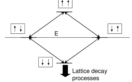
Figure 4: Schematic of levels for a pair of two-level systems with indirect coupling between two degenerate states, augmented with loss. Coupling to the lower state with zero units of excitation leads to a situation in which the state energy (which is close to that of a basis state with one unit of two-level excitation) is much greater than the basis state energy. In the model with loss under discussion, the lattice has the possibility of expressing the energy difference through loss channels. The destructive interference between the upper and lower pathway is now broken.

To augment the model with loss, we adopt a description based on a sector decomposition of the available state space. Processes that preserve sector are described with sector-specific operators that are Hermitian. Processes that remove probability amplitude from one sector to another are described by operators that are not Hermitian with respect to a single sector, but are Hermitian over all sectors. Suppose that we assume that lattice-induced decay processes near 24 MeV involve energetic decay products (such as alpha particles, protons, neutrons, etc.). We could then define our sector of interest as one which lacks any such energetic decay products. We employ an infinite-order Brillouin-Wigner approach to eliminate the sector with energetic decay products, and the loss is accounted for through a non-Hermitian term in the sector Hamiltonian for our sector of interest. The approach is equivalent to that discussed by Feshbach,Feshbach although our application and language are different.

The idealized Hamiltonian is augmented with loss by first restricting it to the sector of interest, and then including decay processes using a loss operator that is anti-Hermitian with respect to the sector. This produces

$$\hat{H}~{}=~{}\Delta E_{1}{\hat{S}_{z}^{(1)}\over\hbar}+\Delta E_{2}{\hat{S}_{z}^{(2)}\over\hbar}+\hbar\omega_{0}\hat{a}^{\dagger}\hat{a}-{i\hbar\over 2}\hat{\Gamma}(E)+V_{1}e^{-G}{2\hat{S}_{x}^{(1)}\over\hbar}(\hat{a}+\hat{a}^{\dagger})+V_{2}{2\hat{S}_{x}^{(2)}\over\hbar}(\hat{a}+\hat{a}^{\dagger})$$ (6)

The loss term in this model may be thought of as arising from second-order terms of the form

$$i~{}{\rm Im}\bigg{\{}\hat{V}[E-\hat{H}_{0}]^{-1}\hat{V}\bigg{\}}$$

which are explicitly dependent on the energy $E$. Loss mechanisms and operators are discussed briefly in Appendix A.

III.2 Excitation transfer in weak coupling

We turn our attention first to the issue of the existence of an excitation transfer effect in this augmented model. Although we are most interested in model systematics in the strong coupling limit, it is convenient here to consider the excitation transfer effect in the weak coupling limit using second-order perturbation theory. The relevant second-order interaction is derived from

$$V_{1}e^{-G}{2\hat{S}_{x}^{(1)}\over\hbar}(\hat{a}+\hat{a}^{\dagger})[E-\hat{H}_{0}]^{-1}V_{2}{2\hat{S}_{x}^{(2)}\over\hbar}(\hat{a}+\hat{a}^{\dagger})~{}+~{}V_{2}{2\hat{S}_{x}^{(2)}\over\hbar}(\hat{a}+\hat{a}^{\dagger})[E-\hat{H}_{0}]^{-1}V_{1}e^{-G}{2\hat{S}_{x}^{(1)}\over\hbar}(\hat{a}+\hat{a}^{\dagger})$$

If we keep near-resonant terms, then we obtain

$$\hat{V}_{12}~{}=~{}V_{1}V_{2}e^{-G}{\hat{S}_{+}^{(1)}\over\hbar}{\hat{S}_{-}^{(2)}\over\hbar}\bigg{(}{\hat{a}^{\dagger}\hat{a}\over\Delta E_{1}+\hbar\omega_{0}+i\hbar\Gamma/2}+{\hat{a}\hat{a}^{\dagger}\over\Delta E_{1}-\hbar\omega_{0}+i\hbar\Gamma/2}-{\hat{a}^{\dagger}\hat{a}\over\Delta E_{2}-\hbar\omega_{0}}-{\hat{a}\hat{a}^{\dagger}\over\Delta E_{2}+\hbar\omega_{0}}\bigg{)}$$

$$~{}+~{}V_{1}V_{2}e^{-G}{\hat{S}_{-}^{(1)}\over\hbar}{\hat{S}_{+}^{(2)}\over\hbar}\bigg{(}{\hat{a}^{\dagger}\hat{a}\over\Delta E_{1}+\hbar\omega_{0}+i\hbar\Gamma/2}+{\hat{a}\hat{a}^{\dagger}\over\Delta E_{1}-\hbar\omega_{0}+i\hbar\Gamma/2}-{\hat{a}^{\dagger}\hat{a}\over\Delta E_{2}-\hbar\omega_{0}}-{\hat{a}\hat{a}^{\dagger}\over\Delta E_{2}+\hbar\omega_{0}}\bigg{)}$$

In this equation, the loss term $\Gamma(E)$ is to be evaluated with a surplus of roughly $\Delta E_{1}$.

If we were to set these loss terms to zero, then we could compare this interaction with what we obtained previously. This is most interesting and relevant on resonance when $\Delta E_{1}=\Delta E_{2}$. In this case the second-order interaction is approximately

$$\hat{V}_{12}~{}\rightarrow~{}{2\hbar\omega_{0}V_{1}V_{2}e^{-G}\over\Delta E^{2}}\left[{\hat{S}_{+}^{(1)}\over\hbar}{\hat{S}_{-}^{(2)}\over\hbar}+{\hat{S}_{-}^{(1)}\over\hbar}{\hat{S}_{+}^{(2)}\over\hbar}\right]\ \ \ \ \ \ \ \ \ \ [\Gamma(E)\rightarrow 0]$$ (7)

This is in agreement with the results obtained using our approximate diagonalization in the previous section.

On the other hand, if the decay rate is enormous we would obtain approximately

$$\hat{V}_{12}~{}\rightarrow~{}-{2V_{1}V_{2}e^{-G}\over\Delta E}(\hat{a}^{\dagger}\hat{a}+\hat{a}\hat{a}^{\dagger})\left[{\hat{S}_{+}^{(1)}\over\hbar}{\hat{S}_{-}^{(2)}\over\hbar}+{\hat{S}_{-}^{(1)}\over\hbar}{\hat{S}_{+}^{(2)}\over\hbar}\right]\ \ \ \ \ \ \ \ \ \ [\Gamma(E)\rightarrow\infty]$$ (8)

The effect of loss in this case is to destroy destructive interference between the different pathways, which leads to a dramatic enhancement of the excitation transfer rate.

IV Energy exchange with the oscillator

We now turn our attention to the energy exchange effect when loss (at the two-level system transition energy) is present. In our study of the lossless version of the problem, we observed that after rotation a self-energy term was present that produced an energy shift, and also an additional term was present that could exchange two units of excitation in association with the transfer of a modest number of oscillator quanta. Based on the above perturbation theory results, in the presence of loss we would expect a much larger self-energy shift and energy exchange effect (even though we do not at present have a simple rotation to bring out the effects so cleanly). We consider in this section first a numerical result in intermediate coupling, and then an analytic result in strong coupling, to illustrate this.

IV.1 Receiver-side self-energy and energy exchange: Intermediate coupling strength

To develop numerical solutions for the lossy case, we require a specific loss model. We have studied energy exchange with a number of different loss models, with the result that once the destructive interference is broken as discussed above, then the self-energy and energy exchange effects are increased dramatically as compared to the lossless case. Relatively minor differences in comparison occur between the results with different loss models. In Appendix B we describe an approximate wavefunction which captures the dominant effect (the elimination of destructive interference from contributions from different paths) by omitting parts of the wavefunction most impacted by loss in a model with loss that increases strongly with energy. Such a model results in a flattening of the wavefunction above a constant energy line in $(n,M_{2})$-space [or a surface in $(n,M_{1},M_{2})$-space]. [The notion of $(n,M_{1},M_{2})$-space is connected with the construction of a solution using $|n\rangle|S_{1},M_{1}\rangle|S_{2},M_{2}\rangle$ product basis states.]

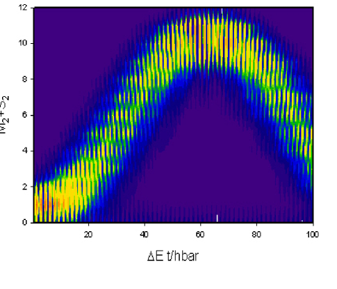
Figure 5: Demonstration of energy exchange between the receiver-side two-level systems and the oscillator in the case of infinitely fast loss. In this calculation, twelve receiver-side two-level systems were included with the oscillator (the coupling with the first set of two-level systems was set to zero). The coupling strength was taken to be $V_{2}\sqrt{n_{0}}/\Delta E=0.4$. The oscillator energy was taken to be $\hbar\omega_{0}=\Delta E_{2}/15$, and we assumed an oscillator excitation near $n_{0}=10^{8}$. In this calculation, the full model sector Hamiltonian with loss was diagonalized, and a dynamical solution was developed through a selection of components localized near the twelve-oscillator ground state. Plotted is the logarithm of the probability distribution for $M_{2}+S_{2}$, which is proportional to the excitation of the receiver-side two-level systems, as a function of time. One observes a very rapid and nearly complete coherent excitation of the two-level systems. The associated probability distribution for the oscillator in this calculation is illustrated in the following figure.

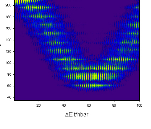
Figure 6: Logarithm of the probability distribution of the oscillator states as a function of time for the calculation described in the previous figure. One sees in this calculation that the energy going into the excitation of the twelve two-level systems is lost from the oscillator.

The results of a calculation based on this kind of approximation illustrating energy exchange between the oscillator and twelve two-level systems is shown in Figures 5 and 6. In the first of these, the probability distribution of the receiver-side two-level systems is shown as a function of time. One observes that energy is transferred to the two-level systems rapidly, much faster (Figure 5) than in the lossless case that we considered above (Figure 3). One observes that the energy increase associated with the excitation of the two-level systems matches the energy loss from the oscillator (Figure 6).

IV.2 Receiver-side self-energy and energy exchange: Strong coupling

In the limit of strong coupling between the oscillator and two-level systems on the receiver side, we are able to develop approximate analytic results. This is discussed in more detail in Appendix C. This approximate model is consistent with the assumption that the oscillator energy can be neglected (which makes the problem approximately periodic locally) to develop an estimate of the local self-energy. The result of this analysis is an approximate self-energy given by

$$E_{2}(\theta)~{}\approx~{}E_{0}-2V_{2}\sqrt{n_{0}}\cos(\theta)\sqrt{S_{2}^{2}-(M_{2})_{0}^{2}}$$ (9)

where $E_{2}$ refers to the energy of the oscillator and the receiver-side two-level systems (the first set of two-level systems being omitted from this calculation), where $E_{0}$ here is the bare energy around which the solution is developed

$$E_{0}~{}=~{}\left[\Delta E_{2}M_{2}+\hbar\omega_{0}n\right]_{(n,M_{2})_{0}}$$ (10)

The phase $\theta$ refers to the local phase in the $e^{in\theta}$ dependence of the solution on $n$ assumed in the approximate local solution. The variable $\theta$ is conjugate to $n$, and can be identified with a wave momentum in the $n$-direction. Associated with this self-energy estimate, we can develop a group velocity estimate given by

$${dn\over dt}~{}\sim~{}{1\over\hbar}{dE_{2}\over d\theta}~{}=~{}{2V_{2}\sqrt{n_{0}}\sin(\theta)\sqrt{S_{2}^{2}-(M_{2})_{0}^{2}}\over\hbar}$$ (11)

In essence, free energy exchange between the oscillator and two-level systems occurs in the strong coupling regime [where the maximum rates occur for $\sin(\theta)=\pm 1$]. This is consistent with the effect seen in the numerical result discussed above for energy exchange in the case of intermediate coupling strength. It is also consistent with more sophisticated results we have obtained using the method outlined in Section VI (but which are not presented explicitly in this paper).

V Excitation transfer

In the weak coupling limit, we have seen that the second-order interaction which is associated with excitation transfer is much increased due to the presence of loss. Once again, we require different tools to study the system when the coupling on the receiver side is of intermediate strength or is strongly coupled (the coupling from the first set of two-level systems in this model will always be weak).

V.1 Excitation transfer: Intermediate coupling strength

We first consider numerical results for the case where the receiver-side coupling is of intermediate strength. In Figures 7 and 8 we show numerical solutions (in the approximation described in Appendix B) for the Schrödinger equation using the model Hamiltonian augmented with loss [Equation (6)] which shows excitation transfer (Figure 7) under conditions where the energy exchange with the oscillator is small (Figure 8). From this calculation, one sees that excitation is transferred from the first set of two-level systems to the second set, with an associated rate which is much faster (Figure 7) than what we found previously in the lossless case (Figure 2).

In the lossless case, we observed that it was important to match the dressed transition energies in order to maximize the effect. Here, the self-energy shift on the receiver side is much greater, and in general it is more difficult to match dressed transition energies. Nevertheless, in the model with loss excitation is transferred even without such a precise matching, due in part to the ability of the two-level systems on the receiver side to exchange energy with the oscillator. Even though we sought to minimize energy exchange with the oscillator in the numerical calculation, one can see a relatively small modulation of the oscillator probability distribution in association with the excitation transfer (Figure 8).

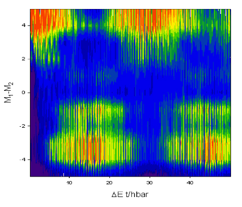
Figure 7: Demonstration of excitation transfer between the first set of two-level systems and the second set of two-level systems in the case of infinitely fast loss. The calculation was performed with two sets of 5 two-level systems, where the undressed energy of the receiver-side system is $\Delta E_{2}=1.01\Delta E_{1}$. The coupling on the donor side is $V_{1}e^{-G}\sqrt{n_{0}}/\Delta E=0.2$, and the coupling on the receiver side is $V_{2}\sqrt{n_{0}}/\Delta E=0.6$. The oscillator energy was taken to be $\hbar\omega_{0}=\Delta E_{1}/27$, and we assumed an excitation level $n_{0}=10^{8}$. In this calculation, the full lossy model Hamiltonian was diagonalized, and a dynamic solution was developed from the eigenstates which shows the excitation transfer effect with relatively small energy exchange with the oscillator. Shown is the logarithm of the probability distribution for $M_{1}-M_{2}$ as a function of time. One observes a fast excitation transfer effect in this case, with most of the excitation being transferred from the first set of two-level systems to the second. The probability distribution associated with the oscillator is shown in the following figure.

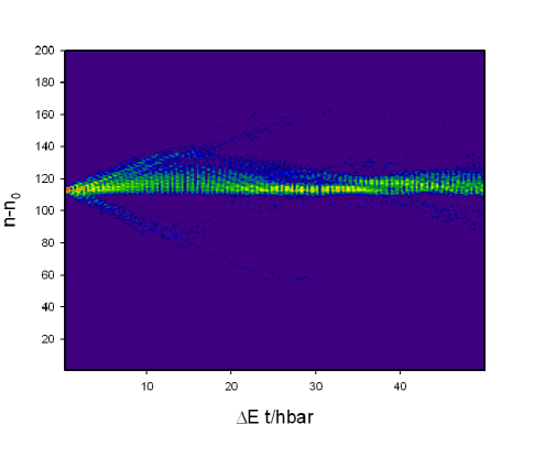
Figure 8: Logarithm of the probability distribution of the oscillator states as a function of time for the calculation described in the previous figure. One sees that there is a small exchange of oscillator energy in association with the excitation transfer effect.

V.2 Excitation transfer: Strong coupling

We consider excitation transfer in the case of strong coupling on the receiver side, and weak coupling on the donor side, in Appendix D. As before, we adopt an approximate solution which depends on the oscillator number $n$ according to $e^{in\theta}$. In addition, we assume a sinusoidal solution $e^{i(M_{2}-M_{1})\phi}$ which depends on the difference between the level of excitation of the two sets of two-level systems. An oscillatory solution of the form $e^{i(M_{2}-M_{1})\phi}$ becomes exact in model in which the coupling terms in the Hamiltonian are taken to be independent of $n$, $M_{1}$, and $M_{2}$, which makes the model periodic in $(n,M_{1},M_{2})$-space as discussed in Section VI. The variable $\phi$ is conjugate to $M_{2}-M_{1}$, and can be identified with the momentum for the coupled system propagating in the $(M_{2}-M_{1})$-direction. In this case, the self-energy is given approximately by

$$E(\theta,\phi)~{}\approx~{}E_{0}+{\Delta E\over 2}-2\sqrt{n_{0}}\cos(\theta)\left[V_{2}\sqrt{S_{2}^{2}-(M_{2})_{0}^{2}}+V_{1}e^{-G}\sqrt{S_{1}^{2}-(M_{1})_{0}^{2}}\cos(2\phi)\right]$$ (12)

where

$$E_{0}~{}=~{}\Delta E_{1}(M_{1})_{0}+\Delta E_{2}(M_{2})_{0}+\hbar\omega_{0}n_{0}$$

and where $\Delta E_{1}=\Delta E_{2}$ appears here as $\Delta E$. The self-energy term from this model is the same as we obtained in the previous section. A new term appears here that is associated with indirect coupling between the two sets of two-level systems. The excitation transfer rate (group velocity) is

$${d\over dt}(M_{2}-M_{1})~{}\sim~{}{1\over\hbar}{dE\over d\phi}~{}=~{}{4V_{1}e^{-G}\sqrt{n_{0}}\cos(\theta)\sin(2\phi)\sqrt{S_{1}^{2}-(M_{1})_{0}^{2}}\over\hbar}$$ (13)

Excitation transfer in this case proceeds freely with a maximum rate occuring when $|\cos(\theta)\sin(2\phi)|=1$.

VI Approximate periodic model and results

We have considered a variety of models including loss at the two-level system energy, and these models exhibit enhanced rates for excitation transfer and energy exchange. In the limit that the oscillator excitation is large (so that $n$ is large), and the number of excited states of the two-level systems is also large, it is possible to develop a different kind of model which takes advantage of the approximate periodicity of the system in $(n,M_{1},M_{2})$-space. The development of periodic solutions in the large $n$ limit has been studied in the closely related spin boson model by Cibils et al.Cibils1991 Calculations of the associated energy band structure leads to results which support the conclusions obtained in the previous sections.

VI.1 Approximate periodic model

In the models under discussion, there are three degrees of freedom corresponding to the oscillator excitation ($n$), and the degree of excitation of the two-level systems ($M_{1},M_{2}$). Energy increases with increasing oscillator number and Dicke number, so that the system cannot be periodic in the direction of increasing energy. However, there are two other directions in which the Hamiltonian is approximately invariant with respect to appropriate translations in $n$, $M_{1}$, and $M_{2}$. If we work with an approximate Hamiltonian with interaction terms that are locally invariant, then this new approximate model is periodic. For example, such an approximate Hamiltonian can be written as

$$\hat{H}~{}=~{}\Delta E_{1}M_{1}+\Delta E_{2}M_{2}+\hbar\omega_{0}n-{i\hbar\over 2}\hat{\Gamma}(E)+\Delta E_{1}g_{1}(\hat{\delta}_{+}^{(1)}+\hat{\delta}_{-}^{(1)})(\hat{\delta}_{+}+\hat{\delta}_{-})+\Delta E_{1}g_{2}(\hat{\delta}_{+}^{(2)}+\hat{\delta}_{-}^{(2)})(\hat{\delta}_{+}+\hat{\delta}_{-})$$ (14)

Here, we have defined two dimensionless coupling constants according to

$$g_{1}~{}=~{}{V_{1}e^{-G}\sqrt{n}_{0}\sqrt{S_{1}^{2}-(M_{1})_{0}^{2}}\over\Delta E_{1}}\ \ \ \ \ \ \ \ \ \ \ \ \ \ g_{2}~{}=~{}{V_{2}\sqrt{n}_{0}\sqrt{S_{2}^{2}-(M_{2})_{0}^{2}}\over\Delta E_{1}}$$ (15)

To correspond with the models under discussion above, the reduced coupling constant $g_{1}$ will be small, and the reduced coupling constant $g_{2}$ will be large. The various $\hat{\delta}$ functions that appear are reduced raising and lowering operators which act according to

$$\hat{\delta}_{\pm}|n\rangle~{}=~{}|n\pm 1\rangle\ \ \ \ \ \ \ \ \ \hat{\delta}_{\pm}^{(1)}|S_{1},M_{1}\rangle~{}=~{}|S_{1},M_{1}\pm 1\rangle\ \ \ \ \ \ \ \ \ \hat{\delta}_{\pm}^{(2)}|S_{1},M_{2}\rangle~{}=~{}|S_{1},M_{2}\pm 1\rangle$$ (16)

This Hamiltonian is invariant under translations of the form

$$\hat{T}_{1}~{}=~{}\hat{\delta}^{(1)}_{-}+{\Delta E_{1}\over\hbar\omega_{0}}\hat{\delta}_{+}\ \ \ \ \ \ \ \ \ \ \hat{T}_{2}~{}=~{}\hat{\delta}^{(2)}_{-}+{\Delta E_{2}\over\hbar\omega_{0}}\hat{\delta}_{+}$$ (17)

as long as $\Delta E_{1}/\hbar\omega_{0}$ and $\Delta E_{2}/\hbar\omega_{0}$ are integers, and also as long as the loss operator is consistent with periodicity.

VI.2 Numerical result

We have used this model to investigate excitation transfer both on, and off, resonance. We would like to confirm the approximate results for excitation transfer that we found in the strong coupling limit in the previous section. In addition, we find that the model predicts fast excitation transfer rates when the energies of the two-level systems are not precisely matched, which is interesting. For the computations discussed here, we have adopted the approximate wavefunction discussed in Appendix B.

We consider a set of calculations done with the periodic model in which the bare receiver-side transition energy is matched to a specific integer number of oscillator quanta

$$\Delta E_{2}=101\,\hbar\omega_{0}$$

and that different combinations of donor-side transition energy and oscillator quanta are matched to the receiver-side transition energy

$$\Delta E_{1}+\Delta n\hbar\omega_{0}~{}=~{}\Delta E_{2}$$

We assume that the two dimensionless coupling strengths are

$$g_{1}=0.01\ \ \ \ \ \ \ \ \ \ \ \ \ \ \ g_{2}=10.0$$

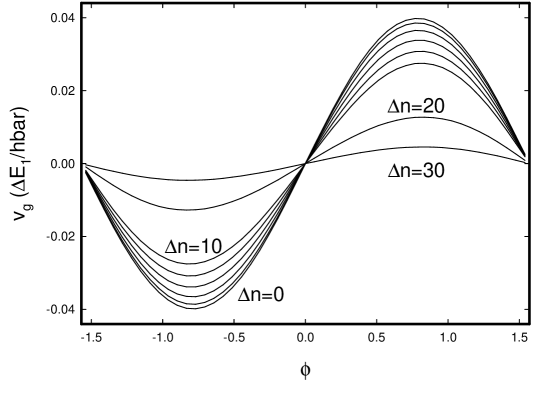
Figure 9: Group velocity calculated for a set of models based on the approximate periodic Hamiltonian discussed in Section VI. In these models, the receiver-side two-level system energy is matched according to $\Delta E_{2}=101\hbar\omega_{0}$, and the donor side is low by an even number of oscillator quanta $\Delta n$ (0, 2, 4, 6, 8, 10, 20, and 30). We have assumed a restricted set of basis states consistent with the approximation discussed in Appendix B, consistent with a loss model that increases rapidly with increasing available energy. We have selected the lowest energy band, corresponding to $\theta\approx 0$, which would be the band with the lowest loss in the case of the dipole coupling model described in Appendix A. Results are shown for the group velocity as a function of $\phi$, using the definition of $\phi$ used in Section 5 and Appendix D.

In a specific calculation, we obtain a moderate number of energy bands which can be understood as originating from an approximate local $e^{in\theta}$ dependence which must match periodic boundary conditions. Within this scheme, one of the bands will have the lowest loss (such as near $\theta=0$ as discussed briefly in Appendix C). Most interesting is the excitation transfer rate computed for the band that corresponds most closely to the $\theta=0$ solution. The lowest energy band corresponds most closely to this solution, and the associated self-energy is close to what we would estimate using the results from the local approximate solution given in the previous sections [Equations (9) and (12)]. We present results for the excitation transfer rate from a set of calculations shown in Figure 9. One sees that the transfer rate on-resonance is very similar to the excitation transfer rate off of resonance. In this case, we see that the energy mismatch between $\Delta E_{1}$ and $\Delta E_{2}$ must be about 14% in order for the excitation transfer rate to drop by a factor of 2 from its maximum value.

VI.3 Comparison with approximate result

We may check the approximate result that we obtained in Appendix D for the maximum excitation transfer rate on resonance against the numerical result presented here. The energy estimate that we obtained in Equation (12) can be written in terms of the dimensionless coupling constants as

$$E(\theta,\phi)~{}=~{}E_{0}+{\Delta E\over 2}-2g_{2}\cos(\theta)\Delta E_{1}-2g_{1}\cos(\theta)\cos(2\phi)\Delta E_{1}$$ (18)

The approximate result for the excitation transfer rate can then be written as

$${d\over dt}(M_{2}-M_{1})~{}\sim~{}4g_{1}\cos(\theta)\sin(2\phi){\Delta E_{1}\over\hbar}$$ (19)

The numerical solution corresponds to $\cos(\theta)=1$, and we have used $g=0.01$. Consequently, the approximate solution evaluates to

$${d\over dt}(M_{2}-M_{1})~{}\sim~{}0.04\,\sin(2\phi){\Delta E_{1}\over\hbar}$$ (20)

This corresponds well with the $\Delta n=0$ result plotted in Figure 9.

The reason that the approximate result works so well in this comparison is that the numerical result corresponds to the periodic model with small (but finite) $\hbar\omega_{0}$ while the approximate result corresponds to zero $\hbar\omega_{0}$.

VII Connection with experiment

The models presented here were developed in response to experiments that appear to show an excess heat effect in metal deuterides. A key feature of these experiments of interest to us is that they seem to present examples of nuclear reactions in which the reaction energy is not expressed as energetic particles, as would be expected in vacuum reactions. In one application of the basic model, the upper and lower levels on the donor side may be molecular D₂ and ⁴He states. If the excitation energy of D₂ relative to ⁴He is transferred elsewhere, such as to highly excited states in Pd, then reaction energy is not expressed in energetic p+t or n+³He channels as occurs in vacuum. Rapid excitation transfer from one site to another in the receiver nuclei would allow the energy to be exchanged coherently with the highly excited phonon mode, or incoherently with other phonon modes, a small number of quanta at a time.

The number of issues associated with such a proposal is quite large, and we do not have the opportunity here to address each of them. We choose to focus here on phonon exchange, and screening as it contributes to estimates of the reaction rate.

VII.1 Phonon exchange

The inclusion of phonon exchange a nuclear reaction matrix element has been discussed previously by Chaudhary and Hagelstein.ChaudHag2006 From this work, one may think about phonon exchange from the point of view of the lattice simply. When two deuterons tunnel sufficiently close for a strong force interaction to occur, together they appear the rest of the lattice as a localized mass 4 and charge 2 object. A direct transition to ⁴He would not be expected to produce significant phonon exchange, since helium also appears to the rest of the lattice as a localized mass 4 and charge 2 object. For phonon exchange to occur, there needs to be a change in the local charge (and hence force constants) or mass. Consequently, we consider a second-order transition in which

$${\rm D}_{2}~{}\leftrightarrow~{}{\rm n}+^{3}{\rm He}~{}\leftrightarrow~{}^{4}{\rm He}$$

In such a second-order transition, we need to sum over contributions from all possible n+³He intermediate states

$$V_{1}(\epsilon)e^{-G}\sqrt{n_{0}}~{}\rightarrow~{}\sum_{j}{\langle\Phi[^{4}{\rm He}]|\hat{V}_{n}|\Phi_{j}[^{3}{\rm He}+{\rm n}]\rangle\langle\Phi_{j}[^{3}{\rm He}+{\rm n}]|\hat{V}_{n}|\Phi[{\rm D}_{2}]\rangle\over(\epsilon-E_{j})}$$ (21)

where $\hat{V}_{n}$ is the strong force interaction operator. Here individual nuclear matrix elements calculated including phonon exchange effects as outlined in Chaudhary and Hagelstein.ChaudHag2006

We would expect to encounter destructive interference in the summation over intermediate n+³He states for off-resonant states, which is equivalent to a localization of the neutron in the vicinity of ³He, and we would not expect to see significant phonon exchange as the virtual n+³He state would also look like a mass 4 charge 2 object to the rest of the lattice. We would expect significant phonon exchange only for n+³He states in which the relative energy is on the order of the vibrational energy of the ³He nucleus associated with the highly excited phonon mode. A schematic (exaggerated) of the corresponding classical trajectories in such a case are illustrated in Figure 10. An analogous deviation of trajectories would be expected for intermediate p+t states; however, we have not included them since at such low relative energies one would expect a tunneling hindrance due to the Coulomb barrier.

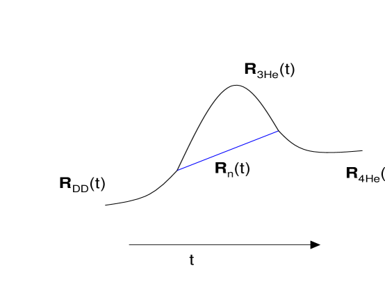
Figure 10: Schematic of classical trajectories corresponding to intermediate states in which the relative neutron and ³He energies are on the order of the ³He oscillation energy due to a highly excited phonon mode. Prior to the first interaction, two deuterons are initially localized with a center of mass location as indicated. After the first interaction, the ³He nucleus sees essentially the same forces but responds with a lighter mass, while the neutron follows a straight line trajectory. Significant contribution to the second-order interaction will only come from such states in which the classical trajectories intersect later on so that there is a likelihood of a second interaction. After the second interaction, the final state ⁴He nucleus follows a trajectory different that followed by the initial localized D₂ center of mass trajectory due to the interaction. The difference in trajectories due to the interactions and separation of the neutron and ³He in the intermediate state corresponds in the classical picture to phonon exchange having occured.

We might expect that the situation on the receiver side should be analogous. Hence, we propose that an initial ground state receiver nucleus makes a phonon-induced indirect transition to a near-resonant excited state by going through intermediate daughter plus neutral states. Only intermediate states of this kind with relative kinetic energy on the order of the local initial vibrational energy would be expected to be able to exchange phonons.

VII.2 Excitation transfer rate and consistency with experiment

Of interest is whether the excitation transfer model can help explain the excess heat effect discussed in the Introduction. To assess this, we face several issues. We require excitation to occur at a rate fast enough so that the associated excitation energy transferred per unit time is predictive of the excess power. We also require that the energy exchange between the excited nuclei on the receiver side occurs fast enough to convert the excitation once transferred, but not so fast that the receiver-side is no longer in the strong coupling regime. In addition, we need an estimate of the hindered coupling strength on the donor side. This is made difficult due to the present situation in which experiment shows clearly screening effects which are not at present matched by theory.

Nevertheless, it is reasonable to embark on the discussion here, in spite of these difficulties. We begin with the ansatz that the energy exchange effect is fast enough that excitation transfer is rate limiting, but slow enough that the system remains in the strong coupling limit. The maximum rate per donor-side two-level system at which excitation transfer can occur in the case of a single mode and single receiver-side excited state in the model is

$$\gamma_{max}~{}=~{}{\left[\displaystyle{1\over 2}\displaystyle{d\over dt}(M_{2}-M_{1})\right]_{max}\over 2S_{1}}~{}=~{}{\left[\displaystyle{2V_{1}e^{-G}\sqrt{n_{0}}\sqrt{S_{1}^{2}-M_{1}^{2}}\over\hbar}\right]_{max}\over 2S_{1}}~{}=~{}{V_{1}e^{-G}\sqrt{n_{0}}\over\hbar}$$ (22)

It seems a reasonable conjecture to assume that concurrent excitation transfer to other excited states should be possible, producing a larger rate for excitation transfer from the excited donor state. It may be the case as well the donor levels could concurrently transfer excitation in association with other highly excited modes. Such effects would further increase the total rate for excitation transfer over the single-mode and single receiver-side excited state estimate. The maximum power that can be associated with the basic single-mode, single receiver-side excited state case is

$$P_{max}~{}=~{}N_{DD}\Delta E_{1}{V_{1}e^{-G}\sqrt{n_{0}}\over\hbar}$$ (23)

where $N_{DD}$ is the number of molecular D₂ states participating. We note that our simple estimate below will be referenced to the ground state, where in a more accurate calculation we should take into account that other rotational and vibrational states will be occupied as well.

Since the tunneling factors are very small, it has proven difficult for any theory to successfully account for the rates associated with the excess heat effect. Consequently, it may be illuminating here to examine a representative example under the assumption that only a single mode and single receiver-side excited state is involved. A variety of experimental and theoretical results leads to the conclusion that it is the near-surface region as being active in a successful Fleischmann-Pons experiment. Calculations on bulk palladium hydrideSun89 ; Liu89 ; Lam89 ; Chris89 ; Wang89 ; Wei90 ; Swit91 indicate that the mean separation between protons is substantially greater than for molecular H₂, so that one would not expect deuterium to be present in states resembling molecular D₂ in the bulk. A simple way to think about this is that molecular D₂ anti-bonding states are occupied in palladium deuteride, which results in the absence of a potential minimum below 1 Å separation.Wei90 Hence, we need to look elsewhere for a suitable host environment, which leads us to the cathode surface where one can typically find dendritic structures produced by codeposition. Codeposition of Pd at high hydrogen or deuterium chemical potential produces a high defect concentration since single site defects are stabilized,Fukai and we conjecture that D₂ in states should occur under conditions where antibonding states do not have such high occupation as in the bulk. We assume for this discussion that the outer 10 microns of the cathode consists of codeposited material with a high defect concentration in which molecular D₂ is present in relatively high concentrations (10^-4), leading to a population $N_{DD}$ on the order of $4\times 10^{15}$ D₂ molecules for a 1 cm² cathode surface area.

We require next a parameterization of the interaction matrix element [realistic calculations based on Equation (21) are in progress]. Two deuterons must tunnel together to interact, which suggests that the interaction matrix element should include a Gamow factor and volume factors according to

$$V_{1}\sqrt{n_{0}}e^{-G}~{}\rightarrow~{}\sqrt{v_{nuc}\over v_{mol}}~{}e^{-G(U_{e})}~{}u_{DD}$$ (24)

where $v_{mol}$ is the relevant volume associated with molecular D₂, and where $v_{nuc}$ is the relevant volume associated with the nucleon distribution when strong force interactions occur (we use $\sqrt{v_{nuc}/v_{mol}}$ to be $8.5\times 10^{-8}$ here). We have written the tunneling factor with an explicit dependence on the screening potential $U_{e}$ in recognition that our result will depend on what screening model is used. The parameter $u_{DD}$ is the residual second-order interaction between two deuterons leading to phonon exchange and ⁴He formation. We adopt a provisional value of 1 MeV for $u_{DD}$.

The tunneling factor in the case of molecular D₂ can be estimated from fusion rate calculations presented in the literatureKoonin ; Shimamura to be about $1.7\times 10^{-36}$. Experiments by the LUNA collaboration on low energy deuteron-deuteron fusion reactions show enhancements in the yield which can be fit through the use of a screening potential $U_{e}$.Raiola2004 ; Rolfs2004 ; Raiola2005 For insulators the screening potential values found are low ($<30$ eV), which is similar to the result for molecular D₂. Screening energies for metals are in the range of 130 eV to 800 eV. The experimental results appears to follow an empirical scaling law based on a Debye screening formula. Czerski et alCzerski have recently published a calculation of the fusion rate per molecule as a function of the screening potential, from which one sees a roughly 30 order of magnitude increase at 100 eV, and 40 order of magnitude increase at 200 eV.

In light of this, we do not have a good estimate for the Gamow factor appropriate to the outer cathode surface region, which makes the task of predicting a reaction rate difficult at this time. However, we can develop a consistency check to see whether the screening parameter required by the model to match the excess heat is consistent with low energy fusion experiments. The largest screening parameter is required under the assumption of a singly highly excited phonon mode, and single receiver-side excited state. We match the excitation transfer rate to a representative excess power, and solve for the screening parameter $U_{e}$

$$N_{DD}\Delta E_{1}\sqrt{v_{nuc}\over v_{mol}}{u_{DD}\over\hbar}~{}e^{-G(U_{e})}~{}=~{}0.3~{}{\rm watt}$$ (25)

Solution of this equation produces a (near zero relative energy) screening energy $U_{e}$ of about 115 eV, which is below the screening energies obtained from (keV relative energy) deuteron-deuteron fusion experiments in metals. According to the modeling of Czerski et alCzerski , one would expect the screening energy to depend on the relative deuteron energy. In a model calculation relevant to PdD, the screening energy at low (1 eV) relative energy ($U_{e}\sim$ 55 eV) is about 60% of the screening energy at high (10 keV) relative energy ($U_{e}\sim$ 90 eV). Experiment for this case is consistent with a screening energy of 800$\pm$90 eV. At present, no model can account for the large screening energies observed experimentally. However, the (near zero relative energy) screening energy $U_{e}$ required here for consistency seems quite plausible.

VII.3 Energy exchange with the lattice

In the model that we have proposed, the initial (slow) excitation transfer is followed by subsequent (fast) excitation transfer reactions among the receiver-side nuclei. With each individual receiver-side excitation transfer reaction there is the possibility of coherent and incoherent phonon exchange with the lattice. We do not have an estimate for the rate of incoherent exchange from this model, but we can compare the coherent rate required with our strong coupling result to assess whether the associated coherent rate is sufficient. To proceed, we form the ratio $r$ of the power associated with excitation transfer and the power associated with energy exchange

$$r~{}=~{}{\left[\displaystyle{\Delta E_{1}\over 2}\displaystyle{d(M_{2}-M_{1})\over dt}\right]\over\left[\hbar\omega_{0}\displaystyle{dn\over dt}\right]}~{}=~{}{\Delta E_{1}\over\hbar\omega_{0}}{V_{1}\over V_{2}}{\sqrt{S_{1}^{2}-M_{1}^{2}}\over\sqrt{S_{2}^{2}-M_{2}^{2}}}\cot(\theta)\sin(2\phi)~{}e^{-G}$$ (26)

In the event that the two powers are matched at the maximum excitation transfer rate [$\sin(2\phi)=1$], then $r=1$, and we may write

$$\tan(\theta)~{}=~{}{\Delta E_{1}\over\hbar\omega_{0}}{V_{1}\over V_{2}}{\sqrt{S_{1}^{2}-M_{1}^{2}}\over\sqrt{S_{2}^{2}-M_{2}^{2}}}~{}e^{-G}$$ (27)

There is no information available from experiment at present as to what phonon mode frequencies are involved. For phonon mode frequencies in the kHz to MHz regime, the combination of the Gamow factor, and volume factor in $V_{1}$, lead to solutions where $\theta$ is very small under most conditions. We conclude from this that in the strong coupling limit the excitation energy can readily be transferred to the oscillator, and that this argument supports the ansatz of the previous subsection.

VIII Summary and conclusions

We considered basic models in which two sets of two-level systems are coupled to a common highly excited oscillator, where the two-level system transition energy is much greater than the oscillator energy. We focused on the case of linear coupling with the oscillator (qualitatively similar results can be obtained with nonlinear coupling). These models exhibit an excitation transfer effect, in which excitation from one set of two-level systems is transferred to the other set. This effect is a consequence of indirect coupling between the two sets of two-level systems. We have demonstrated the existence of this excitation transfer effect through a numerical calculation, and also through approximate diagonalization. We also demonstrated the existence of an energy exchange effect, in which energy from the two-level systems is transferred coherently to the oscillator, even though the energies may be incommensurate. This effect comes about because excitation transfer among the two-level systems occurs in association with oscillator exchange, and coherence can be maintained over the course of many such transfer and exchange processes. Both effects are weak in the lossless case, and require precise resonances between the two-level systems (for excitation transfer), and two-level systems and multiples of the oscillator energy (energy exchange).

We then discussed a version of the model augmented with loss effects at the two-level transition energy. The inclusion of loss changes the problem qualitatively, due to the elimination of destructive interference effects between different pathways involved in coupling between basis states. When loss is present, the rates for excitation transfer and energy exchange are greatly increased (in comparison with the lossless case), and depend weakly on the specific loss model used. Consequently, we have introduced an approximate restricted wavefunction that omits states most strongly impacted by loss for a loss model in which decay rates increase strongly with energy. We take advantage of this approximation to develop numerical and analytic results for the excitation transfer and energy exchange effects. The analytic results developed in the strong coupling limit are in good agreement with results obtained using a periodic model.

These models were developed in response to experiments in which excess heat is observed at levels much greater than can be accounted for by chemical processes, in which no energetic particles are observed. Measurements of ⁴He correlated with the excess energy lead one to conclude that some new kind of nuclear process is involved, and the reaction $Q$-value determined from experiment is about 24 MeV consistent with

$${\rm d}+{\rm d}~{}\to~{}^{4}{\rm He}+24~{}{\rm MeV}~{}{\rm(heat)}$$

This conjecture has been controversial since there have been no previous observations of reactions that work this way in nuclear physics, and because one normally expects the reaction energy to be expressed in terms of energetic particles. However, if the local reaction energy of a deuteron-deuteron reaction can be transferred elsewhere (such as described in the simple models discussed in this paper), then the situation changes. The idealized models described in this paper then correspond to new reaction mechanisms that have not been seen previously in nuclear physics, and which would behave differently.

We examined the reaction rate for excitation transfer in connection with excess heat in a Fleischmann-Pons experiment, and we conclude that theory and experiment can be consistent as long as a strong screening effect is present. Recent experimental work on low-energy deuteron-deuteron fusion reactions have shown such a strong screening effect in metals (but not insulators) in the few keV range, and it seems reasonable to expect that this effect will persist at lower energies.

Appendix A: Loss

We are interested in this appendix in loss mechanisms available to the coupled quantum system (made up of two-level systems for nuclear states and an oscillator for a highly excited phonon mode) near the two-level transition energy and above. We recognize two qualitatively different kinds of decay mechanisms: (1) decay of excited nuclear states associated with the two-level systems; and (2) induced decay processes when the coupled system has allowed decay modes. A presumption that we have made in putting forth a model based on two-level systems is that the nuclear states associated with the levels of the two-level systems are stable at least on a timescale of the excitation transfer dynamics. In the case of molecular D₂, numerous calculations have appeared showing slow decay rates (even with screening at the levels discussion in Section VII).Koonin ; Czerski The issue of which specific states on the receiver side is outside of the scope of this paper; for the purposes of the discussion we assume that suitable reasonably stable excited states exist and can be accessed.

Consequently, our attention here is focused on decay mechanisms available to the coupled quantum system. In Section III, we discuss the use of perturbation theory to obtain an estimate for the coupling associated with excitation transfer in which indirect coupling proceeds through off-resonant basis states with energy eigenvalues much less than the initial and final basis state energy eigenvalues. One would expect such off-resonant states to be able to decay through whatever mechanisms are available at the energy defect (which is the transition energy of the two-level systems, which in our discussion is on the MeV scale). If the coupled system (oscillator and two-level systems) is in a strong coupling regime, then a discussion in terms of basis states of the uncoupled system is not helpful, and we need to think in terms of transitions to accessible lower energy states of the coupled system. In either case, we would expect the coupled system to dissipate a large energy quantum. In this appendix we are interested in specific dissipation mechanisms and models. In the next section we will be concerned with the impact of loss on the wavefunctions.

Decay mechanisms

The major decay mechanisms that we might expect include:

• Induced nuclear decay, in which one or more energetic particles is emitted.

• Induced electron recoil, in which a K-shell electron recoils from a nucleus.

One might conjecture that there should exist another loss mechanism in which a large energy quantum is dissipated through a large number of low energy decays, such as electron promotion, phonon generation, atom ejection, and so forth. In our view, if such a decay path existed, evidence for it should have been seen in association with inner-shell fluorescence experiments and experiments involving conventional nuclear decay. One can make theoretical arguments as to why this kind of effect is unlikely, and so we will focus our discussion on low-order energetic decay mechanisms.

If one unit of transition energy is available, we might expect to lose excited states of the two-level systems to the above decay mechanisms. If the transition energy is great enough (keeping in mind that we may be interested in schemes based on HD where the transition energy is about 5.5 MeV), we may lose lower states as well. Upon reflection, one might also expect to see decays of nuclei that make up the host lattice, since one would expect phonon exchange to occur with the highly excited oscillator in association with an induced disintegration. The reason that we are concerned with such issues is that the specific loss mechanisms end up impacting the wavefunction, as we discuss in Appendix B. In this regard, loss mechanisms for donor or receiver nuclei have similar consequences for the wavefunction of the coupled system. It is then convenient here to consider the donor and receiver nuclei as being minor constituents in a host lattice, and focusing on (energetic) loss mechanisms induced in the host lattice through phonon exchange.

In the introduction, we discussed excess heat experiments as producing excess heat but not producing energetic charged particles. Yet here we are focused on loss mechanisms that involve the production of energetic charged particles, which may seem counter-intuitive. The resolution of this is that in our view the wavefunction seeks to avoid regions of high loss (as discussed further in Appendix B), and by doing so achieves in these models stronger coupling, and faster excitation transfer and energy exchange rates. However, we note that there are many experiments with metal deuterides in which excess heat is not observed, in which a variety of energetic particles are present, and where some of the loss mechanisms under discussion seem to be relevant. A systematic understanding of these loss mechanisms in our view is a prerequisite for a comprehensive understanding of the anomalies.

Phonon exchange

The possibility that the coupled oscillator and two-level system may induce disintegrations or electron recoil in nuclei that make up the host lattice motivates us to consider the issue of phonon exchange and coupling in more detail. We are familiar with the lack of phonon exchange in the Mössbauer effect, as well as the breakdown of the Mössbauer effect when the recoil is strong. Phonon exchange through recoil in the presence of a highly excited phonon mode has been studied.Gupta1974 In the event that the nucleus disintegrates, there should also occur phonon exchange with a highly excited phonon mode. In support of this we consider a lattice with a highly excited phonon mode in which a nuclear disintegration occurs under conditions in which the sudden approximation is valid. In the initial state, the nucleus constitutes part of the lattice, and in the final state the nucleus has broken up and the fragments are ejected. In this case, the lattice has changed, and phonon exchange occurs in association with this lattice change. Phonon exchange in association with a force constant change is sometimes referred in terms of a Duschinsky mechanism,Duschinsky ; Sharp ; Faulkner but the matrix formulation applies on equal footing to a mass change. In the present example, nuclear disintegration in the sudden approximation results in both a local mass change (to zero mass since the nucleus is no longer present) as well as a change in force constants (where there used to be forces, none are present in the final state). Consequently, we consider phonon exchange in the case of induced nuclear disintegration to occur through a Duschinsky mechanism.

Induced alpha decay and fission processes would be expected to behave as a generic disintegration following the arguments above. Induced beta decay processes will involve recoil and force constant change, and fit within the scheme under consideration. Induced K-shell electron recoil (in the non-Mössbauer limit) can produce phonon exchange through the associated nuclear recoil if the electron energy is low, or through atomic displacement if the electron is energetic. In all cases, we would expect the possibility of phonon exchange with a highly excited phonon mode.

Interaction Hamiltonian

As an example, we consider the situation in the case of induced alpha decay and other decay processes involving nuclear fragments. In this case, the development of an interaction Hamiltonian is related to (but simpler than) the approach presented recently by Chaudhary and Hagelstein,ChaudHag2006 since all that happens to the lattice is that a nucleus is lost at one site. In general such a loss will produce coupling to essentially all of the phonon modes, but we are only interested here in whatever coupling occurs with the highly excited mode. We would expect to end up with a single site interaction Hamiltonian of the general form (assuming that the decaying nucleus is not part of either the donor or receiver two-level systems)

$$\hat{U}~{}=~{}\sum_{n,n^{\prime}}\sum_{j,k}|\phi_{n^{\prime}}\rangle|\psi_{k}\rangle U^{kj}_{n^{\prime}n}\langle\psi_{j}|\langle\phi_{n}|$$ (28)

The nuclear states here are denoted by $|\psi\rangle$, and the subscripts $j,k$ range over all relevant initial and final nuclear states. The oscillator states here are denoted by $|\phi\rangle$, and phonon exchange occurs when $n\neq n^{\prime}$.

We note that there should exist coupling matrix elements to essentially all available final states in general, but that energy conservation determines which final state channels are open. This is significant in the present discussion in that we should expect a much different dissipation rate and set of products if the available energy is “low” (for example, 1 MeV) as compared to if it is “high” (for example, 30 MeV). The induced disintegration rate in this regime will increase rapidly with increasing energy as more decay channels open. One would also expect there to be statistical factors present when the energy becomes high enough so that two or more fast decays at different sites is allowed. We draw attention to this here as later on this rapid increase in decay with energy will impact the form of the wavefunction we would expect.

Second-order interactions

The most straightforward way to include this kind of decay into the model Hamiltonian under discussion is through infinite-order Brillouin-Wigner theory, in which one sector is identified in which the nucleus is in the ground state and another sector is identified in which the daughter and fragments are present. In this case, the associated second-order interaction is of the form

$$\hat{W}~{}=~{}\hat{U}[E-\hat{H}_{0}]^{-1}\hat{U}$$ (29)

An interaction appropriate to the idealized (and reduced) model can then be developed by taking the expectation value over the ground state nucleus

$$\langle\psi_{i}|\hat{W}|\psi_{i}\rangle~{}=~{}\langle\psi_{i}|\hat{U}[E-\hat{H}_{0}]^{-1}\hat{U}|\psi_{i}\rangle$$ (30)

Ultimately, we will end up with an interaction of the form

$$\langle\psi_{i}|\hat{W}|\psi_{i}\rangle~{}=~{}\sum_{n,n^{\prime\prime}}|\phi_{n^{\prime\prime}}\rangle W_{n^{\prime\prime}n}\langle\phi_{n}|$$ (31)

This interaction will have a real part associated with the self-energy as well as an imaginary part associated with loss if any loss channels are open. The augmentation of the idealized model to include loss should contain terms of the form

$$-i{\hbar\over 2}\hat{\Gamma}(E)~{}=~{}i\,{\rm Im}\bigg{\{}\sum_{j}\langle\psi_{i}|\hat{W}|\psi_{i}\rangle_{j}\bigg{\}}~{}=~{}-i{\hbar\over 2}\sum_{n,n^{\prime\prime}}|\phi_{n^{\prime\prime}}\rangle\Gamma_{n^{\prime\prime}n}\langle\phi_{n}|$$ (32)

where the summation over $j$ includes all sites at which a disintegration might occur.

In the event that we worked with a model in which the Duschinsky mechanism resulted in single phonon exchange, and the basic interaction $\hat{U}$ becomes proportional to $(\hat{a}+\hat{a}^{\dagger})$, then we would expect the loss to depend on the oscillator operators according to

$$-i{\hbar\over 2}\hat{\Gamma}(E)~{}\sim~{}(\hat{a}+\hat{a}^{\dagger})^{2}$$ (33)

Appendix B: Effect of loss on the states of the system

In this appendix we are interested in the impact of loss on wavefunctions of the coupled system, and in the development of approximate wavefunctions for use in estimating rates for excitation transfer and energy exchange. In the end, we propose an approximate wavefunction in which parts that are most strongly impacted by loss are omitted. The proposal for such an approximation is based on intuition that the probability amplitude arranges itself so as to avoid high-loss regions. We begin by examining this in a simple lossy two-state system.

Two-state model with loss

We consider first the case of two generic quantum states, one lossy and one with no loss, that are coupled. We are interested in seeing what happens under conditions when the loss becomes large. For such a problem, we may write

$$E\left(\begin{array}[]{c}c_{1}\cr c_{2}\cr\end{array}\right)~{}=~{}\left(\begin{array}[]{cc}H_{1}&V\cr V&H_{2}-i\displaystyle{\hbar\over 2}\gamma\cr\end{array}\right)\left(\begin{array}[]{c}c_{1}\cr c_{2}\cr\end{array}\right)$$ (34)

We can solve for $c_{2}$ in terms of $c_{1}$ to find

$$c_{2}~{}=~{}\left[{V\over E-H_{2}+i\displaystyle{\hbar\over 2}\gamma}\right]c_{1}$$ (35)

This can be used to develop a nonlinear eigenvalue equation

$$E~{}=~{}H_{1}+{V^{2}\over E-H_{2}+i\displaystyle{\hbar\over 2}\gamma}$$ (36)

There are two solutions in general. In the event that the loss is large, then the solutions divide up into a low-loss solution and a high-loss solution. For the low-loss solution, we may write

$$c_{2}~{}\rightarrow~{}-i{2V\over\hbar\gamma}c_{1}\ \ \ \ \ \ \ \ \ \ \ \ \ \ \ E~{}\rightarrow~{}H_{1}-i{2V^{2}\over\hbar\gamma}$$ (37)

This is interesting since the probability amplitude for the low-loss solution avoids the high-loss region. The loss associated with the low-loss solution scales as $1/\gamma$ in this limit. Hence, the stronger the loss term, the lower the loss of the coupled system. This kind of behavior is reasonably general, and provides us with some intuition about the more complicated coupled problem that we consider in what follows.

In the high-loss solution, the situation is reversed. In this case the probability amplitude seeks lossy regions, and avoids low-loss regions. These solutions are less interesting to us since in general they decay rapidly, and hence are unlikely to be relevant to the basic effects of interest in this manuscript.

Weak coupling limit with strong loss

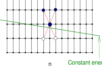
Figure 11: Schematic of wavefunction and constant energy line in the case of one set of two-level systems coupled to an oscillator in the weak coupling limit. Illustrated are the different basis states which appear here as points in $(n,M)$ space. In the weak coupling limit, the wavefunction is composed predominantly of a individual basis state, which we denote here as a enlarged dark circle (that appears at the center of crossed lines). Coupling occurs from this state to neighbors that differ by one unit of $n$ and $M$, which is indicated by four lines originating from the enlarged dark circle, and circles indicating probability amplitude. A constant energy line is illustrated. This constant energy line corresponds to constant $M\Delta E+n\hbar\omega_{0}$ plus a small self-energy shift. Coupling from the center point to the stable states above the constant energy line produce a small probability amplitude in weak coupling, which is indicated as smaller dark circles. Coupling from the center point to the unstable states below the constant energy line produce a much smaller probability amplitude in weak coupling, which is indicated as smaller open circles.

Consider next a model for the receiver side alone with loss, in the limit that the coupling between the two-level systems and oscillator are weak. In this case, we could sensibly work with basis states in $(n,M)$ space that are discrete points, and associate a loss with each point depending on the relevant energy eigenvalue $E$. A schematic of this situation is illustrated in Figure 11. The constant energy line in this figure is

$$E~{}=~{}\Delta EM+\hbar\omega_{0}n+\Sigma(E)$$ (38)

where $\Sigma(E)$ is the self-energy, which is small in weak coupling. The two lower basis states that are reached with linear coupling are below the constant energy line, and we expect these to decay rapidly and hence have a small probability amplitude. Consequently, in the limit where the loss becomes infinite, we would expect that in weak coupling the eigenfunction would be well approximated by the three points above the constant energy line.

Intermediate and strong coupling

To extend our discussion to cases with stronger coupling, we need to rethink how we approach the problem. The reason for this is that we have significant coupling present leading to entanglement between many states, that entanglement is not lost with the energy loss associated with a decay event. This kind of issue has been encountered before in association with loss in the case of quantum optical soliton propagation in a fiber.Fini Photons experience an attractive interaction through the fiber nonlinearity, which counteracts dispersion associated with variations in the index of refraction, to produce correlated many-photon states (optical solitons). Photons are lost when absorbed or scattered by the fiber. When a photon is absorbed, the wavefunction of the remaining system is impacted, leading to increases in the center of mass position and momentum. This leads to quantum noise associated with the optical soliton, and is termed the Gordon-Haus effect. An analysis of this effect in the Schrödinger picture was recently presented by Fini et al.Fini

In this analysis, photon loss is included through matrix elements between initial and final correlated many-photon states which differ in photon number and energy. Underlying this approach is a recognition that most of the correlations present before the decay process will remain after the decay. The situation is similar in the present case. Prior to a decay, we have a coupled system with correlations between the different basis states. After the decay has occurred, the coupled system remains coupled, and whatever correlations were present initially should for the most part still be present. Consequently, the probability of a particular loss event can be determined in terms of initial and final states that include these correlations.

This argument implies that we should calculate the rate of dissipation at a specific energy exchange with a Golden Rule rate formula expressed in terms of eigenfunctions of the coupled system

$$\Gamma(E_{b}-E_{a})~{}=~{}{2\pi\over\hbar}\sum_{j}|\langle\Phi(E_{b})\psi(\epsilon_{b})|\hat{U}|\Phi(E_{a})\psi(\epsilon_{a})\rangle_{j}|^{2}\rho(E_{f})$$ (39)

Here the initial nuclear state at site $j$ is $\psi(\epsilon_{a})$ with energy $\epsilon_{a}$; the final nuclear state after disintegration is $\psi(\epsilon_{b})$ with energy $\epsilon_{b}$. The initial state of the coupled oscillator and two-level systems is $\Phi(E_{a})$ with energy $E_{a}$; the final state of the coupled system is $\Phi(E_{b})$ with energy $E_{b}$. For loss to occur, the coupled system lowers its energy from $E_{a}$ to $E_{b}$, and the nucleus accepts the energy difference, so that

$$\epsilon_{b}~{}=~{}\epsilon_{a}+(E_{b}-E_{a})$$ (40)

The dissipation comes about in this case when two eigenfunctions of the coupled system $\Phi(E_{a})$ and $\Phi(E_{b})$ that have a large energy difference are connected by a low-order phonon operator.

Loss avoidance and approximate wavefunctions

We discussed above the issue of loss avoidance in the presence of strong loss in the case of two generic levels, and we found that the probability amplitude avoided regions of high loss in the case of the low-loss solution. We expect the coupled system composed of a highly excited oscillator and two-level systems to behave similarly. We are interested here in the question of how the coupled system accomplishes this with loss models similar to those considered in Appendix A. From the discussion above, loss can be minimized when the magnitude of the matrix element involved is minimized. In the event that we use a disintegration model based on dipole coupling (as proposed in Appendix A), then this matrix element is proportional to

$$\bigg{\langle}\Phi(E_{b})\bigg{|}\langle\psi(\epsilon_{b})|\hat{U}|\psi(\epsilon_{a})\rangle\bigg{|}\Phi(E_{a})\bigg{\rangle}~{}\sim~{}\bigg{\langle}\Phi(E_{b})\bigg{|}(\hat{a}+\hat{a}^{\dagger})\bigg{|}\Phi(E_{a})\bigg{\rangle}$$ (41)

If the loss increases rapidly with increasing energy (due to enhanced tunneling, opening of new channels, or statistical factors), then the coupled system can minimize loss by reducing the magnitude of such matrix elements when the energy difference $E_{b}-E_{a}$ is large.

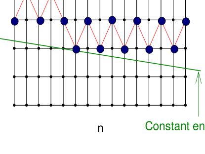
Figure 12: Schematic of wavefunction and constant energy line in the case of one set of two-level systems coupled to an oscillator when loss increases as a strong function of the available energy. This situation corresponds to intermediate coupling, in which the wavefunction includes many points in $(n,M)$ space, which lie above the constant energy line. This constant energy line here again corresponds to constant $M\Delta E+n\hbar\omega_{0}$ plus a self-energy term which we assume is small. Loss is minimized through localization of the wavefunction in $M$, since the coupling between similar eigenfunctions that are offset by two units in $M$ is minimized.

A simple approximation can be developed by working with wavefunctions for which most of these matrix elements are identically zero for an energy exchange of $2\Delta E$ or greater. Such a wavefunction is illustrated in Figure 12. This wavefunction lies above the constant energy line, and is restricted to having only a single nonzero point for each $M$. Such wavefunctions will exhibit no loss for most transitions with $E_{b}-E_{a}\geq 2\Delta E$, but will have loss at lower energy separation. For example, a displacement down by one unit in $M$, and over by one unit in $n$, produces a lower energy wavefunction for which a finite loss matrix element occurs. There is no possibility of a wavefunction construction for which finite coupling is maintained and this kind of loss can be avoided completely. However, the magnitude of the loss for one unit separation in $M$ will depend on the relative phases of the wavefunction in $n$, so that in a subset of the possible solutions this loss will be minimized.

In the case of a single oscillator coupled to two sets of two-level systems, a similar construction is possible in which the wavefunctions lie above and close to the constant energy surface. Such solutions again minimize the loss in the presence of dissipation that increases strongly with energy. In the numerical calculations of the coupled system with a lossy oscillator, we have made use of these kinds of approximate wavefunctions.

Appendix C: Energy exchange with the oscillator

In the models under discussion in the main text, the two-level systems on the receiver side are strongly coupled to the oscillator. This coupling produces a self-energy shift as well as an energy exchange effect with the lattice. In this appendix we develop an approximate solution for the coupled lossy oscillator and two-level systems on the receiver side in order to study energy exchange between the two-level systems and the oscillator. In the presence of loss, the receiver-side sector Hamiltonian is

$$\hat{H}_{2}~{}=~{}\Delta E_{2}{\hat{S}_{z}^{(2)}\over\hbar}+\hbar\omega_{0}\hat{a}^{\dagger}\hat{a}-{i\hbar\over 2}\hat{\Gamma}(E)+V_{2}{2\hat{S}_{x}^{(2)}\over\hbar}(\hat{a}+\hat{a}^{\dagger})$$ (42)

where as before we assume that the oscillator energy $\hbar\omega_{0}$ is small compared to the two-level system energy $\Delta E_{2}$. We are interested in this problem when $n$ is large, when the number of two-level systems is large ($S_{2}\gg 1$), and when there is significant excitation of the two-level systems.

We seek approximate solutions to the associated time-independent Schrödinger equation to gain some understanding of the system dynamics. We adopt a loss model of the kind discussed in Appendix A, with the loss increasing rapidly with increased energy exchange. We adopt approximate solutions that are localized in $M_{2}$ as discussed in Appendix B. The loss in the vicinity of $\Delta E_{2}$ in what follows is taken to be weak (this assumes that the Dicke enhancement factors associated with coherence are large). Although we have studied this kind of problem using both analytic and numerical approaches, a presentation of the results would make this manuscript excessively long. We instead will focus here on an approximate local solution, which appears to capture many important features observed in numerical calculations and analytical work.

Wavefunction solutions in $(n,M_{2})$ space lie above and close to a constant energy line as illustrated in Figure 12 in the model under consideration. In this case, we can develop an approximate local solution of the form

$$\Psi(M_{2},n)~{}=~{}e^{in\theta}\times\left\{\begin{array}[]{cc}-\delta_{M_{2}-M_{0}}&{\rm even}~{}n\cr\delta_{M_{2}-M_{0}-1}&{\rm odd}~{}n\cr\end{array}\right.$$ (43)

where $M_{0}$ is the smallest local value of $M_{2}$ that lies above the constant energy line (we have used even and odd $n$ here to implement solutions that alternate in $n$; similar results are obtained with even and odd reversed here). This solution is to be considered to be local in the sense that we will adopt it only in the vicinity of $(n_{0},M_{0})$. Associated with this local solution is an energy eigenvalue estimate

$$E_{2}(\theta)~{}\approx~{}\Delta E_{2}M_{0}~{}+~{}\hbar\omega_{0}n_{0}~{}-~{}2V_{2}\sqrt{n_{0}}\cos(\theta)\sqrt{S_{2}^{2}-M_{0}^{2}}$$ (44)

For this approximate local solution to be good, we need to be locally in the strong coupling limit

$$2V_{2}\sqrt{n_{0}}\cos(\theta)\sqrt{S_{2}^{2}-M_{0}^{2}}~{}\gg~{}\Delta E_{2}$$ (45)

In the event that dissipation comes about due to dipole coupling as discussed in Appendix A, then the dissipation rate in this model will be proportional to

$$\Gamma(\theta)~{}\sim~{}1-\cos(\theta)$$ (46)

The lowest dissipation then appears when $\theta=0$.

This local solution has given us an estimate of the self-energy associated with rapid excitation transfers in the receiver system in the strong coupling limit. From the dependence of the self-energy on $\theta$, we can determine roughly how fast energy can be exchanged between the oscillator and two-level systems. For example, the associated group velocity for energy exchange with the oscillator in this model is

$${dn\over dt}~{}\sim~{}{1\over\hbar}{dE_{2}\over d\theta}~{}=~{}{2V_{2}\sqrt{n_{0}}\sin(\theta)\sqrt{S_{2}^{2}-M_{0}^{2}}\over\hbar}$$ (47)

This rate can be very fast. The coupled oscillator and two-level systems on the receiver side appear to be capable of efficient coherent energy exchange under conditions where the two quantum systems have incommensurate energy quanta. If the loss is minimized at the value of $\theta$ in which the velocity is zero, as occurs in the simple loss model we considered here, then one would expect to see dissipation in association with the coherent energy exchange.

Appendix D: Excitation transfer

We are interested in this appendix in examining excitation transfer in the strong coupling regime, including the effects of loss. We recall that in the model under discussion, two sets of two-level systems are coupled to a highly excited oscillator. When no loss is present the excitation transfer effect is weak, and it requires that the energies be closely matched (as discussed in the main text). When the model is augmented with loss, the situation changes. The excitation transfer effect is strongly enhanced in the weak coupling regime and intermediate coupling regime as discussed in the main text. We expect that the effect is similarly enhanced in the strong coupling regime, which motivates us to explore a simple local model for excitation transfer here.

We have also seen that the introduction of loss has a strong effect on energy exchange between the two-level systems and oscillator on the receiver side, significantly increasing the strength of the effect. We noted in the case of our numerical results in the intermediate coupling regime that there occured a weak energy exchange effect in association with excitation transfer, such that the oscillator was able to make up the difference between the dressed two-level energies. Here we are interested in the possibility of energy exchange with the oscillator in association with excitation transfer between the two sets of two level systems under conditions where a mismatch occurs.

To investigate these issues, we begin with the model Hamiltonian

$$\hat{H}~{}=~{}\Delta E_{1}{\hat{S}_{z}^{(1)}\over\hbar}+\Delta E_{2}{\hat{S}_{z}^{(2)}\over\hbar}+\hbar\omega_{0}\hat{a}^{\dagger}\hat{a}-{i\hbar\over 2}\hat{\Gamma}(E)+V_{1}e^{-G}{2\hat{S}_{x}^{(1)}\over\hbar}(\hat{a}+\hat{a}^{\dagger})+V_{2}{2\hat{S}_{x}^{(2)}\over\hbar}(\hat{a}+\hat{a}^{\dagger})$$ (48)

We are interested in the development of an approximate local solution in $(n,M_{1},M_{2})$ space. We have discussed loss models in Appendix A, and we introduced an approximate wavefunction that minimizes loss when the loss increases rapidly with increasing energy exchange in Appendix B. When the coupling is weak, this wavefunction consists of a set of points in $(n,M_{1},M_{2})$ space that lie above a constant energy surface

$$E~{}=~{}\Delta E_{1}M_{1}+\Delta E_{2}M_{2}+\hbar\omega_{0}n+\Sigma(E)$$ (49)

When the coupling is strong the self-energy $\Sigma(E)$ may be large, so that the constant energy surface may move away from its weak-coupling location. Nevertheless, a wavefunction in the strong coupling limit would be expected to lie above a surface, and localize close to this surface in order to minimize loss.

We adopt a local solution of the form

$$\Psi(M_{1},M_{2},n)~{}=~{}e^{in\theta}e^{i(M_{2}-M_{1})\phi}\left\{\begin{array}[]{ll}-\cos(\alpha)\delta_{M_{1}+M_{2}-M_{0}}&{\rm even}~{}M_{0},{\rm even}~{}n\cr\sin(\alpha)\delta_{M_{1}+M_{2}-M_{0}-1}&{\rm odd}~{}M_{0}+1,{\rm odd}~{}n\cr\end{array}\right.$$ (50)

This solution is constructed to lie locally above a constant energy surface (when $\Delta E_{1}$ is roughly matched to $\Delta E_{2}$), consistent with the loss-minimizing solution discussed in Appendix B. As before, we consider this solution to be local in the sense that we use it only in the vicinity of a point in $(n,M_{1},M_{2})$ space. An approximate energy eigenvalue can be developed from the solution of the determinantal equation

$$\det\left(\begin{array}[]{cc}E_{0}-E&v_{1}(\theta,\phi)+v_{2}(\theta,\phi)\cr v_{1}^{*}(\theta,\phi)+v_{2}^{*}(\theta,\phi)&E_{0}+\Delta E-E\cr\end{array}\right)~{}=~{}0$$ (51)

We have defined $E_{0}$ according to

$$E_{0}~{}=~{}(\Delta E_{1}M_{1}+\Delta E_{2}M_{2}+\hbar\omega_{0}n)_{0}$$ (52)

We assume that the two-level systems are resonant:

$$\Delta E~{}=~{}\Delta E_{1}~{}=~{}\Delta E_{2}$$ (53)

The interactions $v_{1}$ and $v_{2}$ are given by

$$v_{1}(\theta,\phi)=2\sqrt{n_{0}}\cos(\theta)V_{1}e^{-G}e^{-i\phi}\sqrt{S_{1}^{2}-(M_{1})_{0}^{2}}\ \ \ \ \ \ \ v_{2}(\theta,\phi)=2\sqrt{n_{0}}\cos(\theta)V_{2}e^{i\phi}\sqrt{S_{2}^{2}-(M_{2})_{0}^{2}}$$ (54)

The general formula for $E(\theta,\phi)$ that results is complicated, and not particularly interesting for our present discussion. More interesting is the formula obtained in the limit that the coupling on the receiver-side is strong. In this limit we may write

$$(E_{0}-E)(E_{0}+\Delta E-E)-|v_{2}|^{2}\left(1+{v_{1}\over v_{2}}+{v_{1}^{*}\over v_{2}^{*}}\right)=0$$ (55)

There are two band solutions since this equation is quadratic. We take the lower energy band since it has a negative self-energy, in keeping with the weak coupling limit

$$E(\theta,\phi)~{}\approx~{}E_{0}+{\Delta E\over 2}-|v_{2}|\sqrt{1+{v_{1}\over v_{2}}+{v_{1}^{*}\over v_{2}^{*}}}$$

We can then use a Taylor series approximation to obtain

$$E(\theta,\phi)~{}\approx~{}E_{0}+{\Delta E\over 2}-2\sqrt{n_{0}}\cos(\theta)\left[V_{2}\sqrt{S_{2}^{2}-(M_{2})_{0}^{2}}+V_{1}e^{-G}\cos(2\phi)\sqrt{S_{1}^{2}-(M_{1})_{0}^{2}}\right]$$ (56)

We see in this formula a receiver-side self-energy term which is the same as what we found in Appendix C. In addition, we obtain a new term from which we are able to determine the group velocity associated with excitation transfer.

There are two features of this result that are of interest to us. In the event that the two-level systems on the donor and receiver sides are matched, then the associated rate for coherent excitation transfer between the two sides is

$${d(M_{2}-M_{1})\over dt}~{}\sim~{}{1\over\hbar}{dE\over d\phi}~{}=~{}{4V_{1}e^{-G}\sqrt{n_{0}}\cos(\theta)\sin(2\phi)\sqrt{S_{1}^{2}-(M_{1})_{0}^{2}}\over\hbar}$$ (57)

This result is of interest since it is sufficiently large to be relevant to experiments that show an excess heat effect (excitation transfer from D₂ in this model is assumed to be followed by either coherent or incoherent energy exchange with the lattice). The second reason that this result is of interest to us is that it suggests that we might expect roughly the same rate for excitation transfer if the donor and receiver levels are not precisely matched, since solutions may be oscillatory in both $\phi$ and $\theta$. We recall that in the absence of loss we required a precise resonance since the coupling was weak. The inclusion of loss results in much stronger coupling, and in the limit that the coupling is strong, then the system appears to be able to evolve with its maximum rate even when a precise resonance is absent. This is a dramatic result, and one which we investigate further in Section VI.

References

- (1) P. L. Hagelstein, M. C. H. McKubre, D. J. Nagel, T. A. Chubb, and R. J. Hekman, Condensed Matter Nuclear Science, Proceedings of the 11th International Conference on Cold Fusion, Marseilles, France, Nov. 2004, ed. J. P. Biberian, World Scientific, p. 23 (2006).
- (2) 2004 U.S. Department of Energy Cold Fusion Review, Reviewer Comments, U.S. Department of Energy, 2004 (unpublished).
- (3) J. Huizenga, N. Ramsey, et al., Cold Fusion Research, a Report of the Energy Research Advisory Board to the United States Department of Energy, Department of Energy document DOE/S-0073, November 1989.
- (4) M. B. Cibils, Y. Cuche, V. Marvulle, W. F. Wreszinski, J.-P. Amiet, and H. Beck, J. Phys. A: Math. Gen. 24 1661 (1991).
- (5) P. L. Hagelstein, International Conference on X-ray Lasers and Applications, Kyoto, Sept. 1998; page 255.
- (6) Th. Förster, Discuss. Faraday Soc. 27 7 (1959).
- (7) Resonance Energy Transfer, edited by D. L. Andrews and A. A. Demidov, John Wiley and sons, New York (1999).
- (8) G. Juzeliunas and D. L. Andrews, Phys. Rev. B 50 13371 (1994).
- (9) T. Vorrath and T. Brandes, Phys. Rev. B 68 035309 (2003).
- (10) R. H. Dicke, Phys. Rev. 93 99 (1954).
- (11) M. Wagner, Unitary transformations in solid state physics, North-Holland, New York, (1986). See Section 10, single spin transformations.
- (12) R. D. Jenkins, G. J. Daniels, and D. L. Andrews, J. Chem. Phys. 120 11442 (2004).
- (13) P. L. Hagelstein, Proc. ICCF7 140 (1998).
- (14) P. L. Hagelstein, Bull. APS, 45 235 (2000).
- (15) H. Feshbach, Ann. Phys. 19 287 (1962).
- (16) Z. Sun and D. Tomanek, Phys. Rev. Lett. 63, 59 (1989).
- (17) F. Liu, B. K. Rao, S. N. Khanna, and P. Jena, Solid State Communications 72, 891 (1989).
- (18) P. K. Lam and R. Yu, Phys. Rev. Lett. 63, 1895 (1989).
- (19) O. B. Christensen, P. D. Ditlevsen, K. W. Jacobsen, P. Stolze, O. H. Nielsen, and J. K. Norskov, Phys. Rev. B 40, 1933 (1989).
- (20) X. W. Wang, S. G. Louie, and M. L. Cohen, Phys. Rev. B 40, 5823 (1989).
- (21) S.-H. Wei and A. Zunger, Solid State Communications 73, 327 (1990).
- (22) A. C. Switendeck, J. Less Common Metals 172-174, 1363 (1991).
- (23) Y. Fukai, O. Nobuyuki, Phys. Rev. Lett. 73 1640 (1994).
- (24) S. E. Koonin and M. Nauenberg, Nature 339 690 (1989).
- (25) I. Shimamura, Prog. Theoretical Phys. 82 304 (1989).
- (26) F. Raiola, L. Gang, C. Bonomo, G. Gyurky, M. Aliotta, H. W. Becker, R. Bonetti, C. Broggini, P. Corvisiero, A. D’Onofrio, Z. Fulop, G. Gervino, L. Gianella, M. Junker, P. Prati, V. Roca, C. Rolfs, M. Romano, E. Somorjai, F. Streider, F. Terrasi, G. Fiorentini, K. Langanke, and J. Winter, Eur. Phys. J. A 19 283 (2004).
- (27) C. Rolfs, Prog. Theoretical Phys. Suppl. 154 373 (2004).
- (28) F. Raiola, B. Buchard, Z. Fulop, G. Gyurky, S. Zeng, J. Cruz, A. Di Leva, B. Limata, M. Fonseca, H. Luis, M. Aliotta, H. W. Becker, C. Broggini, A. D’Onofrio, L. Gianlanella, G. Imbriani, A. P. Jesus, M. Junker, J. P. Ribereiro, V. Roca, C. Rolfs, M. Romano, E. Somorjai, F. Streider, and F. Terrasi, J. Phys. G: Nucl. Phys. 31 1141 (2005).
- (29) K. Czerski, A. Huke, P. Heide, and G. Ruprecht, Europhys. Lett. 68 363 (2004).
- (30) A. Gupta and K. R. Reddy, Phys. Rev. B 10 1847 (1974).
- (31) F. Duschinsky, Acta Physicochimica 7 551 (1937).
- (32) T. E. Sharp and H. M. Rosenstock, J. Chem. Phys. 41 3453 (1964).
- (33) T. R. Faulkner and F. S. Richardson, J. Chem. Phys. 70 1201 (1979).
- (34) I. Chaudhary and P. L. Hagelstein, submitted to Phys. Rev. B (2006). ArXiv cond-mat/0606585.
- (35) J. M. Fini, P. L. Hagelstein, and H. A. Haus, Phys. Rev. A 60 2882 (1999).