Comparison of far-from-equilibrium work relations

Abstract

Recent theoretical predictions and experimental measurements have demonstrated that equilibrium free energy differences can be obtained from exponential averages of nonequilibrium work values. These results are similar in structure, but not equivalent, to predictions derived nearly three decades ago by Bochkov and Kuzovlev, which are also formulated in terms of exponential averages but do not involve free energy differences. In the present paper the relationship between these two sets of results is elucidated, then illustrated with an undergraduate-level solvable model. The analysis also serves to clarify the physical interpretation of different definitions of work that have been used in the context of thermodynamic systems driven away from equilibrium.

I Introduction

In recent years there has been considerable interest in the nonequilibrium statistical mechanics of small systems 05BLR . Among the results that have been derived and tested experimentally, the nonequilibrium work theorem CJ97a ; CJ97b ,

$$\left\langle e^{-\beta W}\right\rangle=e^{-\beta\Delta F},$$ (1)

relates fluctuations in the work $W$ performed during a thermodynamic process in which a system is driven away from equilibrium, to a free energy difference $\Delta F$ between two equilibrium states of the system. Here, $\beta$ specifies an inverse temperature, and the angular brackets denote an average over an ensemble of realizations (repetitions) of the process in question pedagogical . Eq. 1 and closely related results Cro99 ; Cro00 ; HuSz01 , along with experimental confirmations Liphardt02 ; Douarche05 ; Collin05 ; Blickle06 , have revealed that equilibrium free energy differences can be determined from distributions of nonequilibrium work values.

The recent progress in this area has drawn attention to a set of earlier papers by Bochkov and Kuzovlev 77BoKu ; 79BoKu ; BK81a ; BK81b , in which the authors had obtained – as one consequence of a more general analysis – the following result:

$$\left\langle e^{-\beta W_{0}}\right\rangle=1.$$ (2)

The angular brackets and inverse temperature $\beta$ appearing here have the same meaning as in Eq. 1, and $W_{0}$ is identified as the work performed on the system.

Although Eqs. 1 and 2 are evidently similar in structure, they are not identical; most notably, $\Delta F$ does not appear, either explicitly or implicitly, in Eq. 2. The precise relationship between these two results has not been clarified in the literature, nor is it immediately obvious from a quick comparison of the original derivations. The aim of the present paper is to fill this gap, first by deriving the two equalities within a single, Hamiltonian framework, and then by illustrating them both using the simple model of a perturbed harmonic oscillator. The conclusions that will emerge from this analysis are summarized by the following three points.

• Eqs. 1 and 2 apply to the same physical situation: a system, initially described by an unperturbed Hamiltonian $H_{0}$, is driven away from equilibrium by the application of a time-dependent perturbation. In principle, a single set of experiments could be used to test both predictions.

• While both $W$ and $W_{0}$ are identified as work (in Refs.CJ97a ; CJ97b and 77BoKu ; 79BoKu ; BK81a ; BK81b , respectively), the two quantities generally differ; see Eq. 15 below. The difference between them amounts to a matter of convention, related to whether we choose to view the perturbation as an external disturbance, or else as a time-dependent contribution to the internal energy of the system.

• For the special case of cyclic processes, in which the perturbation is turned on and then off, Eqs. 1 and 2 are equivalent.

This paper is organized as follows. Section II establishes the Hamiltonian framework and the notation that will be used throughout the paper. In Section III we derive Eqs. 1 and 2 within this framework. Section IV describes an exactly solvable model – a harmonic oscillator driven by a time-dependent external force – that illustrates the validity of these predictions and provides intuition regarding the two definitions of work, $W$ and $W_{0}$. Finally, Section V presents an alternative derivation of Eqs. 1 and 2, by way of a stronger set of results (Eq. 57). The paper concludes with a brief discussion.

II Setup

To carry out a direct comparison between Eqs. 1 and 2, we will use the setup considered in Ref. BK81a . Consider a classical mechanical system with $D$ degrees of freedom, described by coordinates ${\bf q}=(q_{1},\cdots,q_{D})$ and momenta ${\bf p}=(p_{1},\cdots,p_{D})$, and let $z=({\bf q},{\bf p})$ denote a point in the phase space of this system. Consider also a number of external forces $X_{1},X_{2},\cdots$, which are under our direct control. We act on the system by manipulating these forces. The Hamiltonian that describes this system takes the form

$$H(z;X)=H_{0}(z)-\sum_{k}X_{k}\,Q_{k}(z)$$ (3)

(see Eq. 2.2 of Ref. BK81a ), where $Q_{1}(z),Q_{2}(z),\cdots$ denote the variables conjugate to the external forces:

$$Q_{k}=-\frac{\partial H}{\partial X_{k}}.$$ (4)

$H$ is a function on phase space, parametrized by the forces $X=(X_{1},X_{2},\cdots)$. We will refer to $H_{0}$ as the bare, or unperturbed, Hamiltonian, and to $H$ as the full Hamiltonian.

If this system is brought into weak contact with a thermal reservoir at temperature $T$, with the external forces held fixed, then it will relax to an equilibrium state described by the Boltzmann-Gibbs distribution

$$P^{\rm eq}(z;X)=\frac{1}{Z(X)}\exp\left[-\beta H(z;X)\right],$$ (5)

where $\beta=(k_{B}T)^{-1}$. The corresponding classical partition function and free energy are:

$$Z(X)=\int dz\,\exp\left[-\beta H(z;X)\right]\qquad,\qquad F(X)=-\beta^{-1}\ln Z(X).$$ (6)

Now imagine that we subject this system to a thermodynamic process, defined by the following sequence of steps. Prior to time $t=0$, the system is prepared in equilibrium, in the absence of external forces, i.e. at

$$X_{0}=(0,0,\cdots).$$ (7)

The reservoir is then removed. Subsequently, from $t=0$ to a later time $t=\tau$, the external forces are turned on according to some arbitrary but pre-determined schedule, or protocol, $X_{t}$. The microscopic evolution of the system during this interval of time is described by a trajectory $z_{t}$ evolving under Hamilton’s equations,

$$\frac{d{\bf q}}{dt}=\frac{\partial H}{\partial{\bf p}}\qquad,\qquad\frac{d{\bf p}}{dt}=-\frac{\partial H}{\partial{\bf q}},$$ (8)

where $H=H(z;X_{t})$. The protocol $X_{t}$ effectively traces out a curve in “force space”, from the origin (Eq. 7) to some final point $X_{\tau}$. Let $\Delta F$ denote the free energy difference between two equilibrium states – both at the same temperature $T$ – associated with the initial and final forces:

$$\Delta F=F(X_{\tau})-F(X_{0})=-\beta^{-1}\ln\frac{Z(X_{\tau})}{Z(X_{0})}.$$ (9)

By repeatedly subjecting the system to this process – always first preparing the system in equilibrium, and always using the same protocol $X_{t}$ – we generate a number of statistically independent realizations of the process, each characterized by a Hamiltonian trajectory $z_{t}$ describing the microscopic response of the system to the externally imposed perturbation. Angular brackets $\langle\cdots\rangle$ will specify an ensemble average over such realizations.

For a given realization, let us now define $W$ and $W_{0}$ appearing in Eqs. 1 and 2:

$$W_{0} = \int_{0}^{\tau}dt\,\sum_{k}X_{k}(t)\,\dot{Q}_{k}(z_{t})$$ (10a)

$$W = -\int_{0}^{\tau}dt\,\sum_{k}\dot{X}_{k}(t)\,Q_{k}(z_{t}),$$ (10b)

where the dots denote time derivatives, e.g. $\dot{Q}_{k}=(d/dt)Q_{k}(z_{t})$. These two definitions are not equivalent: in general, $W\neq W_{0}$.

To gain some physical insight into these quantities, we rewrite them as follows:

$$W_{0} = \int dt\,X\cdot\dot{Q}=\int X\cdot dQ$$ (11a)

$$W = -\int dt\,\dot{X}\cdot Q=\int dX\cdot\frac{\partial H}{\partial X},$$ (11b)

where $Q=(Q_{1},Q_{2},\cdots)$ is the vector of variables conjugate to the forces $X=(X_{1},X_{2},\cdots)$ (see Eq. 4). The expression for $W_{0}$ is the familiar integral of force versus displacement found in introductory textbooks on mechanics HRW05 , and corresponds to the definition of work used by Bochkov and Kuzovlev (Eq. 2.9 of Ref. BK81a ). By contrast, expressions equivalent to Eq. 11b are often used to define work in discussions of the microscopic foundations of macroscopic thermodynamics Gibbs ; Schrodinger62 ; UhlenbeckFord ; this is the definition that is used in the context of nonequilibrium work theorems (e.g. Eq. 3 of Ref. CJ97a ). While it might seem unusual that two different quantities, $W_{0}$ and $W$, can both be interpreted as the work performed on a system, this ambiguity simply reflects the freedom we have to define what we mean by the internal energy of the system of interest. We discuss this point in some detail in the following two paragraphs.

What is the internal energy of the system when its microstate is $z=({\bf q},{\bf p})$, and the external forces are set at values $X=(X_{1},X_{2},\cdots)$? Eq. 3 suggests two natural ways to answer this question. (i) We can take the internal energy to be given by the value of the bare Hamiltonian, $H_{0}(z)$. From this perspective the system is imagined as a particle in a fixed energy landscape, $H_{0}$; we affect the particle’s energy by varying the forces so as to move it from one region of phase space to another, but the forces $X$ do not themselves appear in the definition of its energy. (ii) Alternatively, we can define the internal energy to be given by the value of the full Hamiltonian, $H=H_{0}-X\cdot Q$. This point of view is captured by imagining an energy landscape that is not fixed, but changes with time as we manipulate the forces $X$. Let us refer to these two alternatives as the (i) exclusive and the (ii) inclusive frameworks, according to whether the term $-X\cdot Q$ is treated as a component of the internal energy of the system.

Now we use the Hamiltonian identity

$$\frac{\partial H}{\partial z}\cdot\frac{dz}{dt}=\frac{\partial H}{\partial{\bf q}}\cdot\frac{\partial H}{\partial{\bf p}}-\frac{\partial H}{\partial{\bf p}}\cdot\frac{\partial H}{\partial{\bf q}}=0$$ (12)

(see Eq. 8) to obtain

$$\frac{d}{dt}H(z_{t};X_{t})=\frac{\partial H}{\partial z}\cdot\frac{dz}{dt}+\frac{\partial H}{\partial X}\cdot\frac{dX}{dt}=\dot{X}\cdot\frac{\partial H}{\partial X}=-\dot{X}\cdot Q,$$ (13)

and therefore

$$\frac{d}{dt}H_{0}(z_{t})=\frac{d}{dt}\left(H+X\cdot Q\right)=X\cdot\dot{Q}.$$ (14)

Comparing with Eq. 11, we see that $W_{0}$ and $W$ are equal to the net changes in the values of $H_{0}$ and $H$, respectively, during the interval of perturbation:

$$W_{0} = \int_{0}^{\tau}dt\,\frac{dH_{0}}{dt}=H_{0}(z_{\tau})-H_{0}(z_{0})$$ (15a)

$$W = \int_{0}^{\tau}dt\,\frac{dH}{dt}=H(z_{\tau};X_{\tau})-H(z_{0};X_{0}).$$ (15b)

Since the system is thermally isolated (i.e. not in contact with a heat reservoir) from $t=0$ to $t=\tau$, it is natural to identify the work performed on it with the net change in its internal energy. With this in mind, Eq. 15 provides a simple interpretation of the difference between $W$ and $W_{0}$. If we adopt the exclusive point of view and take the internal energy to be the value of the bare Hamiltonian $H_{0}$, then $W_{0}$ is the work performed on the system, by the application of external forces that affect its motion in a fixed energy landscape. If we instead choose the inclusive framework, using the full Hamiltonian $H=H_{0}-X\cdot Q$ to define the internal energy of the system, then $W$ is the appropriate definition of work. The distinction between these two frameworks is illustrated with a specific example in Section IV.

From Eq. 15 we obtain an explicit expression for the difference between $W$ and $W_{0}$:

$$W_{0}-W=X_{\tau}\cdot Q(z_{\tau})=\sum_{k}X_{k}(\tau)\,Q_{k}(z_{\tau}),$$ (16)

since $X_{0}=(0,0,\cdots)$.

III Derivations

Let us now compute the averages of $e^{-\beta W_{0}}$ and $e^{-\beta W}$, over an ensemble of realizations of the thermodynamic process described above. Since the system evolves under deterministic (Hamiltonian) equations of motion from $t=0$ to $t=\tau$, a given realization is uniquely determined by the initial conditions $z_{0}$. We can therefore express $\langle e^{-\beta W_{0}}\rangle$ as an integral over an equilibrium distribution of initial conditions:

$$\left\langle e^{-\beta W_{0}}\right\rangle=\int dz_{0}\,P^{\rm eq}(z_{0};X_{0})\,e^{-\beta W_{0}(z_{0})},$$ (17)

where $W_{0}(z_{0})$ denotes the value of $W_{0}$ for the trajectory launched from the microstate $z_{0}$. The first factor in the integrand is

$$P^{\rm eq}(z_{0};X_{0})=\frac{1}{Z(X_{0})}\,e^{-\beta H_{0}(z_{0})}$$ (18)

[note that $H(z_{0};X_{0})=H_{0}(z_{0})$, by Eq. 7]. Using Eq. 15a, we have

$$W_{0}(z_{0})=H_{0}\left(z_{\tau}(z_{0})\right)-H_{0}(z_{0}),$$ (19)

where $z_{\tau}(z_{0})$ indicates the final microstate of this trajectory, expressed as an explicit function of the initial microstate. Upon substituting these expressions into Eq. 17, a cancellation of terms occurs in the exponents, and we get

$$\left\langle e^{-\beta W_{0}}\right\rangle=\frac{1}{Z(X_{0})}\int dz_{0}\,e^{-\beta H_{0}(z_{\tau}(z_{0}))}.$$ (20)

Since there is a one-to-one correspondence between the initial and final conditions of a given trajectory, we can change the variables of integration from $z_{0}$ to $z_{\tau}$:

$$\left\langle e^{-\beta W_{0}}\right\rangle=\frac{1}{Z(X_{0})}\int dz_{\tau}\left|\frac{\partial z_{\tau}}{\partial z_{0}}\right|^{-1}\,e^{-\beta H_{0}(z_{\tau})}.$$ (21)

We have inserted the determinant of the Jacobian matrix associated with this change of variables. By Liouville’s theorem, this factor is identically unity, $|\partial z_{\tau}/\partial z_{0}|=1$, which finally gives us

$$\left\langle e^{-\beta W_{0}}\right\rangle=\frac{1}{Z(X_{0})}\int dz_{\tau}\,e^{-\beta H_{0}(z_{\tau})}=1,$$ (22)

by Eq. 6.

The exponential average of $W$ (rather than $W_{0}$) follows from similar manipulations:

$$\left\langle e^{-\beta W}\right\rangle = \int dz_{0}\,P^{\rm eq}(z_{0};X_{0})\,e^{-\beta W(z_{0})}$$ (23)

$$= \frac{1}{Z(X_{0})}\int dz_{0}\,e^{-\beta H(z_{\tau}(z_{0});X_{\tau})}$$

$$= \frac{1}{Z(X_{0})}\int dz_{\tau}\,e^{-\beta H(z_{\tau};X_{\tau})}=\frac{Z(X_{\tau})}{Z(X_{0})}=e^{-\beta\Delta F}.$$

We have used $W(z_{0})=H(z_{\tau}(z_{0});X_{\tau})-H(z_{0};X_{0})$ (Eq. 15b) to get from the first line to the second, and a change of variables, $z_{0}\rightarrow z_{\tau}$, to get to the third.

Eq. 22 was originally obtained by Bochkov and Kuzovlev 77BoKu ; 79BoKu ; BK81a ; BK81b , whereas Eq. 23 is the nonequilibrium work theorem of Refs. CJ97a ; CJ97b . These results apply to two physically distinct quantities, $W_{0}$ and $W$, corresponding to different conventions for defining the internal energy of the system. In each case the exponential average of work reduces to a ratio of partition functions. In Eq. 22 the ratio is $Z(X_{0})/Z(X_{0})$, i.e. unity; while in Eq. 23 it is $Z(X_{\tau})/Z(X_{0})$, which yields the free energy difference $\Delta F$.

Let us now consider the special case in which the external forces vanish both at $t=0$ and at $t=\tau$:

$$X_{0}=X_{\tau}=(0,0,\cdots).$$ (24)

This corresponds to a cyclic process, for which the Hamiltonian begins and ends at $H_{0}$. In this case we have, identically, $W=W_{0}$ (Eq. 16) and $\Delta F=0$ (Eq. 6). Thus, Eqs. 22 and 23 are equivalent when the Hamiltonian is varied cyclically.

Finally, it is instructive to consider a process during which the external forces are switched on suddenly at $t=0$, from $X_{0}=(0,0,\cdots)$ to $X_{\tau}=(X_{1},X_{2},\cdots)$. Since the process occurs instantaneously ($\tau\rightarrow 0$), the system has no opportunity to evolve, hence $z_{\tau}=z_{0}$. Thus, Eq. 15 gives us

$$W_{0}=0\qquad,\qquad W=\Delta H(z_{0}),$$ (25)

where $\Delta H(z)\equiv H(z;X_{\tau})-H(z;X_{0})$. Eq. 22 is immediately satisfied, and Eq. 23 reduces to Zwanzig’s perturbation formula zwanzig ,

$$\langle e^{-\beta\Delta H}\rangle_{0}=e^{-\beta\Delta F},$$ (26)

where $\langle\cdots\rangle_{0}$ denotes an average over microstates sampled from the $X=(0,0,\cdots)$ canonical distribution.

IV Example

Figure 1: Distributions of work values $W_{0}$ and $W$ for the harmonic oscillator example, with $\chi=m=\omega=1.0$ and $k_{B}T=0.3$. The distribution $\rho$ is a delta-function at $\Delta F=-0.5$, while $\rho_{0}$ is a Gaussian whose mean is at $-\Delta F$.

Let us now illustrate the general analysis presented above, using the example of a one-dimensional harmonic oscillator perturbed by a uniform external force. We take the bare Hamiltonian

$$H_{0}(z)=\frac{1}{2m}p^{2}+\frac{m\omega^{2}}{2}q^{2},$$ (27)

and we consider a perturbation

$$-XQ(z)=-Xq.$$ (28)

Thus, $H=H_{0}-Xq$. The perturbation describes a force $X$ acting along the direction of the coordinate $q$. The canonical distribution at a given force $X$ is

$$P^{\rm eq}(z;X)=\frac{1}{Z(X)}\exp\left[-\beta(H_{0}-Xq)\right],$$ (29)

and by direct evaluation of Eq. 6 we get

$$F(X)=F(0)-\frac{X^{2}}{2m\omega^{2}}.$$ (30)

Now imagine a process during which the perturbing force is linearly ramped up from zero to some positive value $\chi$:

$$X_{t}=\frac{\chi t}{\tau}\quad,\quad 0\leq t\leq\tau.$$ (31)

To simplify the calculations below, we take $\tau$ to be the period of the unperturbed oscillator:

$$\tau=\frac{2\pi}{\omega}.$$ (32)

The evolution of the system satisfies Hamilton’s equations,

$$\dot{q}=\frac{p}{m}\qquad,\qquad\dot{p}=-m\omega^{2}q+\frac{\chi t}{\tau},$$ (33)

which can readily be solved. For initial conditions $(q_{0},p_{0})$, we get a trajectory

$$q_{t} = q_{0}\cos(\omega t)+\frac{p_{0}}{m\omega}\sin(\omega t)+\frac{\chi}{m\omega^{3}\tau}\left[\omega t-\sin(\omega t)\right]$$ (34a)

$$p_{t} = p_{0}\cos(\omega t)-m\omega q_{0}\sin(\omega t)+\frac{\chi}{\omega^{2}\tau}\left[1-\cos(\omega t)\right],$$ (34b)

hence

$$q_{\tau}=q_{0}+\frac{\chi}{m\omega^{2}}\qquad,\qquad p_{\tau}=p_{0}.$$ (35)

The quantities $W_{0}$ and $W$ then follow from Eq. 15:

$$W_{0}=\chi q_{0}-\Delta F\qquad,\qquad W=\Delta F,$$ (36)

where

$$\Delta F=F(\chi)-F(0)=-\frac{\chi^{2}}{2m\omega^{2}}.$$ (37)

From Eq. 36 we obtain explicit expressions for the distributions of work values, $\rho_{0}(W_{0})$ and $\rho(W)$, assuming initial conditions $(q_{0},p_{0})$ sampled from equilibrium. Since $W=\Delta F$ for every realization, we have

$$\rho(W)=\delta\left(W-\Delta F\right).$$ (38)

In turn, since $W_{0}$ is a linear function of $q_{0}$ (Eq. 36), which is sampled from a thermal, Gaussian distribution with mean $\langle q_{0}\rangle=0$ and variance $\sigma_{q_{0}}^{2}=(m\omega^{2}\beta)^{-1}$, it follows that $W_{0}$ is also distributed as a Gaussian, with mean and variance $\langle W_{0}\rangle=-\Delta F$, $\sigma_{W_{0}}^{2}=\chi^{2}\sigma_{q_{0}}^{2}$. Explicitly,

$$\rho_{0}(W_{0})=\sqrt{\frac{m\omega^{2}\beta}{2\pi\chi^{2}}}\exp\left[-\frac{m\omega^{2}\beta}{2\chi^{2}}\left(W_{0}+\Delta F\right)^{2}\right].$$ (39)

It is now straightforward to verify by inspection and Gaussian integration that Eqs. 1 and 2 are satisfied:

$$\left\langle e^{-\beta W}\right\rangle = \int dW\,\rho(W)\,e^{-\beta W}=e^{-\beta\Delta F}$$ (40)

$$\left\langle e^{-\beta W_{0}}\right\rangle = \int dW_{0}\,\rho_{0}(W_{0})\,e^{-\beta W_{0}}=1.$$ (41)

The very simple expressions obtained above for $W_{0}$ and $W$ are consequences of our choice for $\tau$, Eq. 32. The model remains solvable for arbitrary $\tau$; in that case both $\rho$ and $\rho_{0}$ are Gaussian distributions, satisfying Eqs. 1 and 2, but the expressions for their means and variances are more complicated.

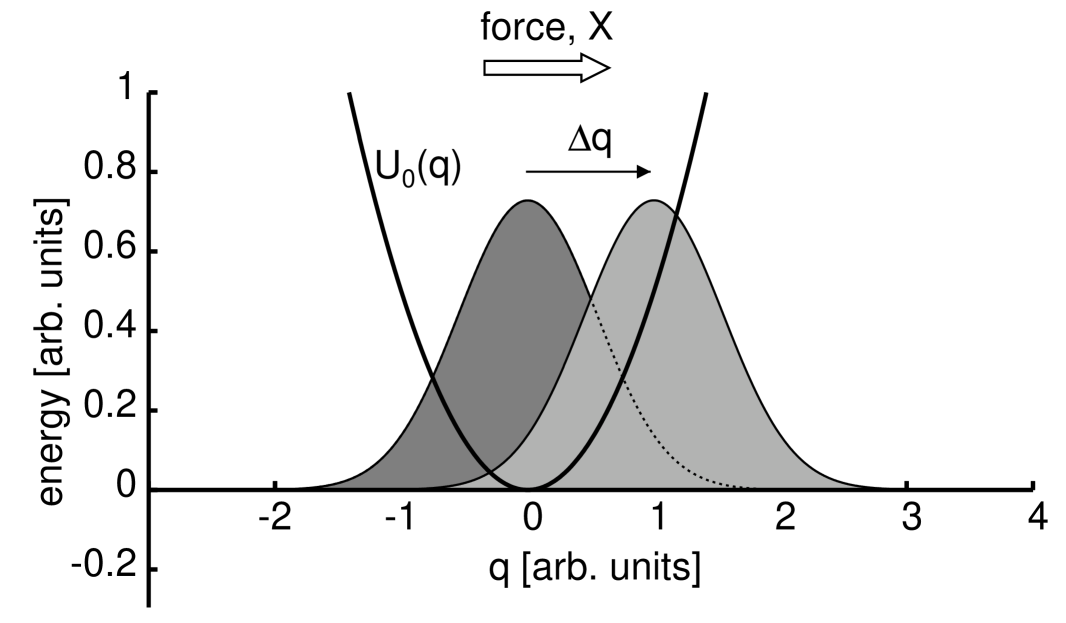
Figure 2: The bare harmonic potential $U_{0}$ is shown, along with the distributions of initial particle positions (dark gray) and final particle positions (light gray). As we turn on the force $X$, we shift the distribution by an amount $\Delta q=\chi/m\omega^{2}=1.0$ away from the minimum of the potential, resulting in an average increase in the value of $U_{0}$.

Fig. 1 depicts the distributions $\rho_{0}$ and $\rho$. Note that $W$ is negative, while the mean value of $W_{0}$ is positive. We can understand this sign difference as follows. Suppose we adopt the exclusive convention and take the internal energy of the system to be given by $H_{0}$. We imagine that the particle evolves in a fixed harmonic well

$$U_{0}(q)=m\omega^{2}q^{2}/2,$$ (42)

under the influence of a time-dependent external force $X_{t}$. The initial position $q_{0}$ is sampled from a Gaussian distribution centered at $q=0$, and as we turn on the perturbing force from $0$ to $\chi$, we displace the particle rightward by a net amount $\Delta q=q_{\tau}-q_{0}=\chi/m\omega^{2}$ (Eq. 35). The final condition $q_{\tau}$ is then distributed as a Gaussian whose mean no longer coincides with the center of the fixed harmonic well, but rather has shifted by a distance $\Delta q$, as shown in Fig. 2. In effect, the perturbation pushes the particle distribution rightward along the $q$-axis, and “up” the quadratic potential energy landscape, resulting in a positive value for the average work, $\langle W_{0}\rangle>0$.

Figure 3: Same as Fig. 2, only now we think in terms of a time-dependent potential well rather than an externally applied force. From $t=0$ to $t=\tau$ the minimum of the harmonic well moves along the path depicted by the thick dashed line. During a given realization, the particle suffers a net displacement $q_{\tau}-q_{0}=\Delta q$, hence $W=U_{\tau}(q_{\tau})-U_{0}(q_{0})=\Delta F$.

Now suppose that we instead choose the inclusive convention and use the full Hamiltonian $H=H_{0}-Xq$ to define the internal energy of the system. Thus we imagine a particle moving in a time-dependent potential,

$$U_{t}(q)=U_{0}(q)-X_{t}q=\frac{m\omega^{2}}{2}\left(q-\frac{\Delta q}{\tau}\,t\right)^{2}+\Delta F\cdot\frac{t^{2}}{\tau^{2}},$$ (43)

where $\Delta q=\chi/m\omega^{2}$ and $\Delta F=-\chi^{2}/2m\omega^{2}$, as above. Eq. 43 describes a harmonic well that moves rightward along the $q$-axis with a velocity $\Delta q/\tau$, and slides downward in energy, as depicted in Fig. 3. We can now appreciate why $W=\Delta F$ for every realization of the process. From $t=0$ to $t=\tau$ the particle moves by a net amount $\Delta q$; simultaneously, the well shifts by the same amount, and acquires an energy offset $\Delta F$:

$$U_{\tau}(q)=\frac{m\omega^{2}}{2}(q-\Delta q)^{2}+\Delta F.$$ (44)

The particle thus ends with the same displacement relative to the minimum of the well as it began with, so the net change in its energy is just the offset $\Delta F$.

In summary, in the exclusive framework, we picture a particle that is pushed rightward by an external force in a fixed harmonic well ($\langle W_{0}\rangle>0$); while in the inclusive framework we imagine a particle that is dragged rightward in space and “downward” in energy by a moving harmonic well ($W<0$).

V Weighted Distributions

Here we sketch an alternative derivation of Eqs. 1 and 2.

Consider an ensemble of realizations of the process described in Section II. Let us picture this ensemble as a swarm of Hamiltonian trajectories evolving in phase space, represented by a density 

$$f(z,t)=\Bigl{\langle}\delta\left(z-z_{t}\right)\Bigr{\rangle},$$ (45)

which satisfies the Liouville equation,

$$\frac{\partial f}{\partial t}=\{H,f\}.$$ (46)

Here we use the convenient Poisson bracket notation: $\{A,B\}=({\partial A}/{\partial{\bf q}})\cdot({\partial B}/{\partial{\bf p}})-({\partial A}/{\partial{\bf p}})\cdot({\partial B}/{\partial{\bf q}})$ . In general, Eq. 46 does not yield a simple solution; the evolution of $f(z,t)$ can be very complicated, particularly if the underlying Hamiltonian dynamics are chaotic.

For a given trajectory $z_{t}$, let

$$w_{0}(t)=\int_{0}^{t}dt^{\prime}\,\sum_{k}X_{k}(t^{\prime})\,\dot{Q}_{k}(z_{t^{\prime}})$$ (47)

denote the amount of work performed on the system to time $t$, using the definition of work corresponding to the exclusive framework (Eq. 10a and Refs. 77BoKu ; 79BoKu ; BK81a ; BK81b ). Since the rate of change of the observable $Q_{k}$ along a trajectory $z_{t}$ is given by $\dot{Q}_{k}=\{Q_{k},H\}$ Goldstein.9.5 , we can rewrite Eq. 47 as

$$w_{0}(t)=\int_{0}^{t}dt^{\prime}\,\{X\cdot Q,H\}=\int_{0}^{t}dt^{\prime}\,\{X\cdot Q,H_{0}\}.$$ (48)

The last equality follows from the identity $\{X\cdot Q,X\cdot Q\}=0$ . Now consider a weighted phase space density

$$g_{0}(z,t)=\Bigl{\langle}\delta\left(z-z_{t}\right)\,\exp[-\beta w_{0}(t)]\Bigr{\rangle},$$ (49)

in which each trajectory carries a statistical weight, $\exp[-\beta w_{0}(t)]$ (see the discussion below). This density satisfies

$$\frac{\partial g_{0}}{\partial t}=\{H,g_{0}\}-\beta\{X\cdot Q,H_{0}\}g_{0},$$ (50)

where the second term on the right accounts for the evolving statistical weights. The derivation of this equation is very similar to those found in Section II of Ref. CJ97b and Section 4.1 of Ref. Ladek .

Since $w_{0}(0)=0$ identically, and since we assume our ensemble is initially prepared in equilibrium, we have $g_{0}(z,0)=f(z,0)=P^{\rm eq}(z;X_{0})$. Given these initial conditions, the unique solution of Eq. 50 is the time-independent distribution

$$g_{0}(z,t)=\frac{1}{Z(X_{0})}\exp[-\beta H_{0}(z)]=P^{\rm eq}(z;X_{0}).$$ (51)

To see this, note that

$$\{H,e^{-\beta H_{0}}\}=-\beta\{H,H_{0}\}\,e^{-\beta H_{0}}=\beta\{X\cdot Q,H_{0}\}e^{-\beta H_{0}},$$ (52)

using the derivative rule for Poisson brackets, and the identity $\{H_{0},H_{0}\}=0$. From this result it follows by inspection that Eq. 51 satisfies Eq. 50.

The functions $f(z,t)$ and $g_{0}(z,t)$ are two different statistical representations of the same ensemble of realizations. Continuing to picture this ensemble as a swarm of trajectories evolving in phase space, $f$ (Eq. 45) can be viewed as a number density, which simply counts how many trajectories are found in the vicinity of $z$ at time $t$; while $g_{0}$ (Eq. 49) can be interpreted as a mass density, if we imagine that each realization carries a fictitious, time-dependent mass $\exp[-\beta w_{0}(t)]$. Eq. 51 then has the following interpretation: when the initial conditions are sampled from equilibrium, the “mass density” of trajectories remains constant in time, even as the “number density” evolves in a possibly complicated way. Thus while the number of trajectories found near a given point $z$ changes with time, these fluctuations are balanced by the evolving statistical weights (fictitious masses) of those trajectories, in precisely such a way as to keep the local mass density constant.

We can obtain analogous results in the inclusive framework (Eq. 10b and Refs. CJ97a ; CJ97b ). Introducing

$$w(t)=-\int_{0}^{t}dt^{\prime}\,\sum_{k}\dot{X}_{k}(t^{\prime})\,Q_{k}(z_{t^{\prime}})=-\int_{0}^{t}dt^{\prime}\,\dot{X}\cdot Q,$$ (53)

along with the corresponding weighted density

$$g(z,t)=\Bigl{\langle}\delta\left(z-z_{t}\right)\,\exp[-\beta w(t)]\Bigr{\rangle},$$ (54)

we obtain the equation of motion CJ97b ; Ladek

$$\frac{\partial g}{\partial t}=\{H,g\}+\beta\dot{X}Qg.$$ (55)

For initial conditions $g(z,0)=f(z,0)=P^{\rm eq}(z;X_{0})$, the unique solution is

$$g(z,t)=\frac{1}{Z(X_{0})}\exp[-\beta H(z;X_{t})]=\frac{Z(X_{t})}{Z(X_{0})}\,P^{\rm eq}(z;X_{t}).$$ (56)

The weighted density is no longer constant in time (as was the case with $g_{0}$), but rather is proportional to the equilibrium distribution corresponding to the current value of the parameters $X$.

The results just obtained are summarized as follows:

$$\Bigl{\langle}\delta\left(z-z_{t}\right)\,\exp[-\beta w_{0}(t)]\Bigr{\rangle} = P^{\rm eq}(z;X_{0})$$ (57a)

$$\Bigl{\langle}\delta\left(z-z_{t}\right)\,\exp[-\beta w(t)]\Bigr{\rangle} = \frac{Z(X_{t})}{Z(X_{0})}\,P^{\rm eq}(z;X_{t}).$$ (57b)

Eqs. 1 and 2 now follow immediately by evaluating Eq. 57 at $t=\tau$ and integrating both sides over phase space. While the derivations presented here are less elementary than those of Section III, we ultimately gain a stronger set of results. By a simple trick of statistical reweighting, we transform an equation of motion that we cannot solve (Eq. 46) into one that is easily solved (Eq. 50 or 55). The result, Eq. 57, allows us to reconstruct equilibrium distributions $P^{\rm eq}$ using trajectories driven away from equilibrium.

Eqs. 57a and 57b are in fact equivalent. Multplying both sides of Eq. 57a by $\exp[+\beta X_{t}\cdot Q(z)]$ and pulling this factor inside the angular brackets, we obtain Eq 57b. Conversely, multiplication by $\exp[-\beta X_{t}\cdot Q(z)]$ leads us from Eq. 57b to Eq. 57a. However, this equivalence is lost once we integrate over phase space: Eqs. 1 and 2 do not imply one another.

Eq. 57b can be viewed as a direct consequence of the Feynman-Kac theorem; this observation by Hummer and Szabo serves as a starting point for their method of reconstructing equilibrium potentials of mean force from single-molecule manipulation experiments carried out away from equilibrium HuSz01 . Moreover, Eq. 57a is essentially a special case of Eq. 12 of Ref. HuSz01 (with $W_{0}$ as generalized by Eq. 59 below), if we assume that their confining potential is initially turned off: $u(z,0)=0$. For an alternative approach to estimating potentials of mean force from similar experiments, see the “clamp-and-release” method proposed by Adib Adib06 .

VI Discussion

The nonequilibrium work theorem, Eq. 1, has generated interest (and controversy CohenMauzerall04 ; CohenMauzerall05 ; Sung.condmat0506214v2 ) primarily for two reasons. First, along with the fluctuation theorem for entropy production 93ECM ; 94ES ; 95GC ; 98Kur ; 99LS ; FT , it is one of relatively few equalities in statistical physics that apply to systems far from thermal equilibrium. Note that the term “fluctuation theorem” has also been used to specify a relation between the response of a system to external perturbations, and a correlation function describing fluctuations of the unperturbed system Hanggi78 ; HanggiThomas82 . Second, Eq. 1 predicts that equilibrium free energy differences can be determined from irreversible processes, counter to expectations that irreversible work values can only place bounds on $\Delta F$ RMA01 . Eq. 2 shares the first feature – it remains valid far from equilibrium – but not the second; it does not seem to be the case that $\Delta F$ can be determined solely from a distribution of values of $W_{0}$.

A crucial distinction in this paper has been the difference between the quantities $W$ and $W_{0}$. The recognition that, in the literature, various meanings are assigned to the term work, might at first come as an unwelcome surprise. Work is a concept of such central importance in thermodynamics that it ought to be unambiguously defined! However, in dealing with a physical situation that involves the mechanical perturbation of a system, the perturbation is inevitably accomplished by coupling externally controlled variables ($X_{1},X_{2},\cdots$) to generalized system coordinates ($Q_{1},Q_{2},\cdots$). This coupling is represented by a term of the form $-\sum_{k}X_{k}Q_{k}$ (or a nonlinear generalization thereof, see below) in the full Hamiltonian that governs the evolution of the system and its surroundings. We are then faced with the question of whether or not to view this term as part of the internal energy of the system of interest. As stressed in this paper, either choice is perfectly acceptable – this is a question of book-keeping rather than principle – but it is precisely this freedom that leads to the ambiguity in the definition of work. For related discussions of this issue, particularly in the context of interpretation of experimental data, see Refs. Sch03 ; Nar04 ; Dha05 ; Douarche05 .

Throughout this paper it has been assumed, following Refs. 77BoKu ; 79BoKu ; BK81a ; BK81b , that the coupling between the forces $X$ and the observables $Q$ is linear: $H=H_{0}-X\cdot Q$. However, as already observed by Bochkov and Kuzovlev, this assumption can easily be relaxed. Had we written the Hamiltonian as

$$H(z;X)=H_{0}(z)-h(Q;X),$$ (58)

and assumed $h(Q;X_{0})=0$, then the entire analysis leading to Eqs. 1 and 2 would have remained valid, provided the following definitions of work:

$$W=-\int_{0}^{\tau}dt\,\dot{X}\cdot\frac{\partial h}{\partial X}\qquad,\qquad W_{0}=\int_{0}^{\tau}dt\,\dot{Q}\cdot\frac{\partial h}{\partial Q}.$$ (59)

We recover Eqs. 3 and 11 with a linear perturbation $h=X\cdot Q$.

While the analysis here has been carried out using Hamiltonian dynamics, the conclusions remain valid under other frameworks for modeling the evolution of the system. The connection to the stochastic approach taken in Ref. HuSz01 has already been noted. Moreover, Eqs. 33 and 34 of Ref. Nar04 , derived for inertial Langevin dynamics, are equivalent to Eqs. 1 and 2 of the present paper. For non-inertial (overdamped) Langevin dynamics, similar results follow directly from the Onsager-Machlup expressions for path-space distributions OM53 ; Dean .

Finally, recall the Crooks fluctuation theorem Cro99 ,

$$\frac{\rho_{F}(+W)}{\rho_{R}(-W)}=\exp[\beta(W-\Delta F)],$$ (60)

where the subscripts refer to two thermodynamic process (forward and reverse) that are related by time-reversal of the protocol used to perturb the system. The Bochkov-Kuzovlev papers contain results that are reminiscent of Eq. 60, for instance Eq. 7 of Ref. 77BoKu and Eq. 2.12 of Ref. BK81a . However, while Crooks uses a definition of work corresponding to $W$ of the present paper, Bochkov and Kuzovlev use $W_{0}$, and their results do not involve $\Delta F$. Moreover, in Refs. 77BoKu ; 79BoKu ; BK81a ; BK81b the derivations seem to assume that the initial conditions are sampled from the same, unperturbed equilibrium distribution for both the forward and the reverse process (see e.g. Eq. 2.6 of Ref. BK81a ). Crooks, by contrast, assumes that the forward and reverse processes are characterized by different initial equilibrium states. It would be useful to clarify more precisely the relationship between these sets of results.

References

- (1) C. Bustamante, J. Liphardt, and F. Ritort, Physics Today 58, 43 (2005).
- (2) C. Jarzynski, Phys. Rev. Lett. 78, 2690 (1997).
- (3) C. Jarzynski, Phys. Rev. E 56, 5018 (1997).
- (4) For pedagogical derivations of Eq. 1 and related results, see for instance Section 7.4.1 of D. Frenkel and B. Smit, Understanding Molecular Simulation: from Algorithms to Applications, second edition, Academic Press, San Diego, 2002; or S. Park and K. Schulten, J. Chem. Phys. 120, 5946 (2004); or G. Hummer and A. Szabo, Acc. Chem. Res. 38, 504 (2005).
- (5) G.E. Crooks, Phys. Rev. E 60, 2721 (1999).
- (6) G.E. Crooks, Phys. Rev. E 61, 2361 (2000).
- (7) G. Hummer, A. Szabo, PNAS 98, 3658 (2001).
- (8) J. Liphardt et al., Science 296, 1832 (2002).
- (9) F. Douarche, S. Ciliberto, A. Petrosyan, and I. Rabbiosi, Europhys. Lett. 70, 593 (2005).
- (10) D. Collin et al., Nature 437, 231 (2005).
- (11) V. Blickle et al, Phys. Rev. Lett. 96, 070603 (2006).
- (12) G.N. Bochkov and Yu.E. Kuzovlev, Zh.Eksp.Teor.Fiz. 72, 238 (1977) [Sov.Phys.–JETP 45, 125 (1977)].
- (13) G.N. Bochkov and Yu.E. Kuzovlev, Zh.Eksp.Teor.Fiz. 76, 1071 (1979) [Sov.Phys.–JETP 49, 543 (1979)].
- (14) G.N. Bochkov and Yu.E. Kuzovlev, Physica 106A, 443 (1981).
- (15) G.N. Bochkov and Yu.E. Kuzovlev, Physica 106A, 480 (1981).
- (16) D. Halliday, R. Resnick, and J. Walker, Fundamentals of Physics, seventh edition, John Wiley and Sons, 2005.
- (17) J.W. Gibbs, Elementary Principles in Statistical Mechanics. Scribner’s, New York, 1902. Pages 42-44.
- (18) E. Schrödinger’s, Statistical Thermodynamics. Cambridge, 1962. See the paragraphs found between Eqs. 2.13 and 2.14.
- (19) G.E. Uhlenbeck and G.W. Ford, Lectures in Statistical Mechanics. Americal Mathematical Society, Providence, 1963. Chapter I, Section 7.
- (20) R. Zwanzig, J. Chem. Phys. 22, 1420 (1954).
- (21) C. Jarzynski, in Lecture Notes in Physics 597, Springer Verlag, Berlin, 2002, eds. P.Garbaczewski and R.Olkiewicz.
- (22) H. Goldstein, Classical Mechanics, 2nd ed., Chapter 9.5. Addison-Wesley, Reading, Massachusetts, 1980.
- (23) A.B. Adib, J. Chem. Phys. 124, 144111 (2006).
- (24) E.G.D. Cohen and D. Mauzerall, J. Stat. Mech.: Theor. Exp. P07006 (2004).
- (25) E.G.D. Cohen and D. Mauzerall, Mol. Phys. 103, 2923 (2005).
- (26) J. Sung, cond-mat/0506214v2 (2005).
- (27) D.J. Evans, E.G.D. Cohen, G.P. Morris, Phys.Rev.Lett. 71, 2401-2404 (1993).
- (28) D. Evans, D. Searles, Phys. Rev. E 50, 1645 (1994).
- (29) G. Gallavotti, E.G.D. Cohen, Phys.Rev.Lett. 74, 2694-2697 (1995).
- (30) J. Kurchan, J.Phys.A 31, 3719 (1998).
- (31) J.L. Lebowitz, H. Spohn, J. Stat.Phys. 95, 333 (1999).
- (32) See also numerous references in D.J. Evans and D. Searles, Adv. Phys. 51, 1529 (2002).
- (33) P. Hänggi, Helv. Phys. Acta 51, 202 (1978).
- (34) P. Hänggi and H. Thomas, Phys. Rep. 88, 207 (1982).
- (35) W.P. Reinhardt, M.A. Miller, and L.M. Amon, Acc. Chem. Res. 34, 607 (2001).
- (36) J.M. Schurr and B.S. Fujimoto, J. Phys. Chem. B 107, 14007 (2003).
- (37) O. Narayan and A. Dhar, J. Phys. A 37, 63 (2004).
- (38) A. Dhar, Phys. Rev. E 71, 036126 (2005).
- (39) L. Onsager and S. Machlup, Phys. Rev. 91, 1505 (1953).
- (40) R. Dean Astumian, personal correspondence and cond-mat/0608352 (2006).