Critical behavior of repulsive dimers on square lattices at $2/3$ monolayer coverage

Abstract

Monte Carlo simulations and finite-size scaling theory have been used to study the critical behavior of repulsive dimers on square lattices at $2/3$ monolayer coverage. A “zig-zag” (ZZ) ordered phase, characterized by domains of parallel ZZ strips oriented at $\pm 45^{o}$ from the lattice symmetry axes, was found. This ordered phase is separated from the disordered state by a order-disorder phase transition occurring at a finite critical temperature. Based on the strong axial anisotropy of the ZZ phase, an orientational order parameter has been introduced. All the critical quantities have been obtained. The set of critical exponents suggests that the system belongs to a new universality class.

I Introduction

The study of critical phenomena and phase transitions is a major and long standing topic in statistical physics.  Stanley ; Fisher ; Kawasaki ; Baxter ; Yeomans ; Goldenfeld ; Domb Particularly, the two-dimensional lattice-gas model Hill with repulsive interactions between the adparticles has received considerable theoretical and experimental interest because it provides the theoretical framework to study structural order-disorder transitions occurring in many adsorbed monolayer films. Dash ; Taub ; Somorjai ; Schick1 ; Binder0 ; Binder1 ; Landau1 ; Binder2 ; Landau2 ; Landau3 ; Schick2 ; Schick3 ; Schick4 ; Patrykiejew Most studies have been devoted to adsorption of particles with single occupancy. The problem becomes considerably difficult when particles occupy two adjacent lattice sites (dimers). Consequently, there have been a few studies devoted to order-disorder transitions associated to dimer adsorption with repulsive lateral interactions. Among them, the structural ordering of interacting dimers has been analyzed by A. J. Phares et al. Phares The authors calculated the entropy of dimer on semi-infinite $M\times N$ square lattice ($N\rightarrow\infty$) by means of transfer matrix techniques. They concluded that there are a finite number of ordered structures. As it arose from simulation analysis, SURFSCI3 only two of the predicted structures survive at thermodynamic limit. In fact, in Ref. SURFSCI3, , the analysis of the phase diagram for repulsive nearest-neighbor interactions on a square lattice confirmed the presence of two well-defined structures: a $c(4\times 2)$ ordered phase at $\theta=1/2$ and a “zig-zag” (ZZ) order at $\theta=2/3$, being $\theta$ the surface coverage.

The thermodynamic implication of such a structural ordering was demonstrated through the analysis of adsorption isotherms, LANG5 the collective diffusion coefficient SURFSCI2 and the configurational entropy LANG6 of dimers with nearest-neighbor repulsion. Later, Monte Carlo (MC) simulations and finite-size scaling (FSS) techniques have been used to study the critical behavior of repulsive linear $k$-mers in the low-coverage ordered structure (at $\theta=1/2$). PRB4 ; PRB5 A ($2k\times 2$) ordered phase, characterized by alternating lines, each one being a sequence of adsorbed $k$-mers separated by $k$ adjacent empty sites, was found. The critical temperature and critical exponents were calculated. The results revealed that the system does not belong to the universality class of the two-dimensional Ising model. The study was extended to triangular lattices. PRB6 In this case, the exponents obtained for $k>1$ and $\theta=k/(2k+1)$ are very close to those characterizing the critical behavior of $k$-mers ($k>1$) on square lattices at $\theta=1/2$.

Recently, by using MC simulations and finite-scaling techniques, Rżysko and Borówko have studied a wide variety of systems in presence of multisite-occupancy. BORO1 ; BORO2 ; BORO3 ; BORO5 ; BORO4 Among them, attracting dimers in the presence of energetic heterogeneity; BORO1 heteronuclear dimers consisting of different segments A and B adsorbed on square lattices; BORO2 ; BORO3 ; BORO5 and trimers with different structures adsorbed on square lattices. BORO4 In these leading papers, a rich variety of phase transitions was reported along with a detailed discussion about critical exponents and universality class.

Summarizing, although there have been various studies for monolayers at half coverage, to the author’s knowledge, there are no conclusive studies on the characteristics of the transition phase of repulsive dimers on a square lattice at $2/3$ coverage. In the present contribution we attempt to remedy this situation. For this purpose, extensive MC simulations in the canonical ensemble complemented by analysis using FSS techniques have been applied. The FSS study has been divided in two parts. Namely, $1)$ a conventional FSS in terms of the normalized scaling variable $\epsilon\equiv T/T_{c}-1$, Fisher ; Binder0 ; Privman ; Privman1 where $T_{c}$ is the critical temperature; and $2)$ an extended FSS,  GARTENHAUS ; CAMPBELL where $\sigma\equiv 1-T_{c}/T$, instead of $\epsilon$, is used. Our results led the determination of the critical temperature separating the transition between a disordered state and the ZZ ordered phase occurring at $2/3$ coverage and the critical exponents characterizing the phase transition.

The outline of the paper is as follows: In Sec. II we describe the dimer lattice-gas model. The order parameter and the simulation scheme are introduced in Secs. III and IV, respectively. Finally, the results and general conclusions are presented in Sec. V.

II The model

In this section, the lattice-gas model for dimer adsorption is described. The surface is represented as a simple square lattice in two-dimensions consisting of $M=L\times L$ adsorptive sites, where $L$ is the size of the system along each axis. The homonuclear dimer is modelled as $2$ monomers at a fixed separation, which equals the lattice constant $a$. In the adsorption process, it is assumed that each monomer occupies a single adsorption site and the admolecules adsorb or desorb as one unit, neglecting any possible dissociation. The high-frequency stretching motion along the molecular bond has not been considered here.

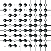
Figure 1: Snapshot of the ordered phase for dimers at $\theta=2/3$.

In order to describe the system of $N$ dimers adsorbed on $M$ sites at a given temperature $T$, let us introduce the occupation variable $c_{i}$ which can take the following values: $c_{i}=0$ if the corresponding site is empty and $c_{i}=1$ if the site is occupied. Under this consideration, the Hamiltonian of the system is given by,

$$H=w\sum_{\langle i,j\rangle}c_{i}c_{j}-Nw+\epsilon_{o}\sum_{i}c_{i}$$ (1)

where $w$ is the nearest-neighbor (NN) interaction constant which is assumed to be repulsive (positive),$\langle i,j\rangle$ represents pairs of NN sites and $\epsilon_{o}$ is the energy of adsorption of one given surface site. The term $Nw$ is subtracted in Eq. (1) since the summation over all the pairs of NN sites overestimates the total energy by including $N$ bonds belonging to the $N$ adsorbed dimers.

III Order parameter

Given the inherent anisotropy of the adparticles, it is convenient to define a related order parameter. In this section, we will briefly refer to a recently reported order parameter $\delta$, PRB5 which measures the orientation of the admolecules in the ordered structure.

Fig. 1 shows one of the possible configurations of the ordered ZZ structure appearing for dimers at $2/3$ monolayer. Though the degeneracy of this phase is high, the entropy per lattice site tends to zero in the thermodynamic limit LANG6 . The figure suggests a simple way to build an order parameter. In fact, any realization of the ZZ structure implies the orientation of the particles along one of the lattice axis. foot1 Then, all the available configurations can be grouped in two sets, according to this orientation. Taking advantage of this property, we define the order parameter as:

$$\delta=\left|\frac{N_{v}-N_{h}}{N}\right|$$ (2)

where $N_{v}$ ($N_{h}$) represents the number of dimers aligned along the vertical (horizontal) axis and $N=N_{v}+N_{h}$.

When the system is disordered $(T>T_{c})$, the two orientations (vertical or horizontal) are equivalent and $\delta$ is zero. As the temperature is decreased below $T_{c}$, the dimers align along one direction and $\delta$ is different from zero. Thus, $\delta$ appears as a proper order parameter to elucidate the phase transition.

IV Monte Carlo method

The lattices were generated fulfilling the following conditions:

• The sites were arranged in a square lattice of side $L$ ($M=L\times L$), with conventional periodic boundary conditions.

• Because the surface was assumed to be homogeneous, the interaction energy between the adsorbed dimer and the atoms of the substrate $\epsilon_{o}$ was neglected for sake of simplicity.

• In order to maintain the lattice at $2/3$ coverage, $\theta=2N/M=2/3$, the number of dimers on the lattice was fixed as $N=M/3$.

• Appropriate values of $L$ ($=60,72,84,96,108$) were used in such a way that the ZZ adlayer structure is not altered by boundary conditions.

In order to study the critical behavior of the system, we have used an exchange MC method. Hukushima ; Earl As in Ref.  Hukushima, , we build a compound system that consists of $m$ noninteracting replicas of the system concerned. The $i$-th replica is associated with a heat bath at temperature $T_{i}$ [or $\beta_{i}=1/(k_{B}T_{i})$, $k_{B}$ being the Boltzmann constant]. To determine the set of temperatures, $\{T_{i}\}$, we set the highest temperature, $T_{1}$, in the high-temperature phase where relaxation (correlation) time is expected to be very short and there exists only one minimum in the free energy space. On the other hand, the lowest temperature, $T_{m}$, is set in the low-temperature phase whose properties we are interested in. Finally, the difference between two consecutive temperatures, $T_{i}$ and $T_{i+1}$ with $T_{i}>T_{i+1}$, is set as $\Delta T=\left(T_{1}-T_{m}\right)/(m-1)$ (equally spaced temperatures).

Under these conditions, the algorithm to carry out the simulation process is built on the basis of two major subroutines: replica-update and exchange.

Replica-update: Interchange vacancy-particle and diffusional relaxation. The procedure is as follows: (a) One out of the $m$ replicas is randomly selected (for example the $i$-th replica). (b) A dimer and a pair of nearest-neighbor empty sites, both belonging to the replica chosen in (a), are randomly selected and their coordinates are established. Then, an attempt is made to interchange its occupancy state with probability given by the Metropolis rule,  Metropolis :

$$P=\min\left\{1,\exp\left(-\beta_{i}\Delta H\right)\right\}$$ (3)

where $\Delta H$ is the difference between the Hamiltonians of the final and initial states. (c) A dimer is randomly selected. Then, a displacement is attempted (following the Metropolis scheme), by either jumps along the dimer axis or reptation through a $90^{o}$ rotation of the dimer axis, where one of the dimer centers remains in its position (interested readers are referred to Fig.  1 in Ref.  SURFSCI2, for a more complete description of the reptation mechanism). This procedure (diffusional relaxation) must be allowed in order to reach equilibrium in a reasonable time.

Exchange: Exchange of two configurations $X_{i}$ and $X_{i^{\prime}}$, corresponding to the $i$-th and $i^{\prime}$-th replicas, respectively, is tried and accepted with probability $W\left(X_{i},\beta_{i}|X_{i^{\prime}},\beta_{i^{\prime}}\right)$. In general, the probability of exchanging configurations of the $i$-th and $i^{\prime}$-th replicas is given by,  Hukushima

$$W\left(X_{i},\beta_{i}|X_{i^{\prime}},\beta_{i^{\prime}}\right)=\left\{\begin{array}[]{cc}1&{\rm for}\ \ {\Delta\leq 0}\\ \exp(-\Delta)&{\rm for}\ \ {\Delta>0}\end{array}\right.$$ (4)

where $\Delta=\left(\beta_{i}-\beta_{i^{\prime}}\right)\left[H(X_{i^{\prime}})-H(X_{i})\right]$. As in Ref.  Hukushima, , we restrict the replica-exchange to the case $i^{\prime}=i+1$.

The complete simulation procedure is the following:

• Initialization.

• Replica-update.

• Exchange.

• Repeat from step 2) $m\times M$ times. This is the elementary step in the simulation process or Monte Carlo step (MCS).

The initialization of the compound system of $m$ replicas, step 1), is as follows. By starting with a random initial condition, the configuration of the replica $1$ is obtained after $n_{1}$ MCS^′ at $T_{1}$ (MCS^′ consists of $M$ realizations of the replica-update subroutine). Second, for $i=\{2,....,m\}$, the configuration of the $i$-th replica is obtained after $n_{1}$ MCS^′ at $T_{i}$, taking as initial condition the configuration of the replica to $T_{i-1}$. This method results more efficient than a random initialization of each replica.

The procedure 1)-4) is repeated for all lattice sizes. For each lattice, the equilibrium state can be well reproduced after discarding the first $n_{2}$ MCS. Then, averages are taken over $n_{MCS}$ successive MCS. As it was mentioned above, a set of equally spaced temperatures is chosen in order to accurately calculate the physical observables in the close vicinity of $T_{c}$.

The thermal average $\langle...\rangle$ of a physical quantity $A$ is obtained through simple averages:

$${\langle A\rangle}=\frac{1}{n_{MCS}}\sum_{t=1}^{n_{MCS}}A\left[X_{i}(t)\right].$$ (5)

In the last equation, $X_{i}$ stands for the state of the $i$-th replica (at temperature $T$). Thus, the specific heat $C$ (in $k_{B}$ units) is sampled from energy fluctuations:

$$\frac{C}{k_{B}}=\frac{1}{(Lk_{B}T)^{2}}[\langle H^{2}\rangle-\langle H\rangle^{2}].$$ (6)

The quantities related with the order parameter, such as the susceptibility $\chi$, and the reduced fourth-order cumulant $U$ introduced by Binder,  Binder2 are calculated as:

$$\chi=\frac{L^{2}}{k_{B}T}[\langle\delta^{2}\rangle-\langle\delta\rangle^{2}]$$ (7)

and

$$U=1-\frac{\langle\delta^{4}\rangle}{3\langle\delta^{2}\rangle^{2}}.$$ (8)

Finally, in order to discuss the nature of the phase transition, the fourth-order energy cumulant, $U_{E}$, was obtained as:

$$U_{E}=1-\frac{\langle H^{4}\rangle}{3\langle H^{2}\rangle^{2}}$$ (9)

Table 1: Parameters used in the MC runs. For all lattice sizes we have chosen $T_{1}=0.25$ and $T_{m}=0.15$ (the temperatures are in units of $w/k_{B}$).

$L$	$m$	$n_{1}$	$n_{2}$	$n_{MCS}$
$60$	$101$	$10^{5}$	$10^{5}$	$3$ x $10^{5}$
$72$	$121$	$10^{5}$	$10^{5}$	$3$ x $10^{5}$
$84$	$141$	$2$ x $10^{5}$	$2$ x $10^{5}$	$5$ x $10^{5}$
$96$	$161$	$4$ x $10^{5}$	$4$ x $10^{5}$	$8$ x $10^{5}$
$108$	$141$	$5$ x $10^{5}$	$5$ x $10^{5}$	$10^{6}$

V Results and conclusions

The critical behavior of the present model has been investigated by means of the computational scheme described in the previous section and FSS techniques. The values of the parameters used in each MC run are shown in Table I. In addition, all the simulation calculations were obtained by averaging over $50$ MC runs.

Because the replica temperatures were chosen equally spaced, the acceptance probability of the replica-exchange decreases in the critical temperature region, reaching a minimum whose value is always greater than $50\%$. The equilibration has been tested by studying how the results vary when the simulation times $n_{2}$ and $n_{MCS}$ are successively increased by factors of $2$. We require that the last three results for all observables agree within error bars. This simple method is shown to be useful to test equilibration [see, for instance, Ref. KATZ, ]. All calculations were carried out using the parallel cluster BACO of Universidad Nacional de San Luis, Argentina. This facility consists of 60 PCs each with a 3.0 GHz Pentium-4 processor.

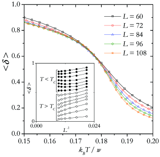
Figure 2: (Color online) Size dependence of the order parameter as a function of temperature. Inset: dependence of $\langle\delta\rangle$ on $L^{-1}$ for different regimes of $T$ as indicated. The error in each measurement is smaller that the size of the symbols.

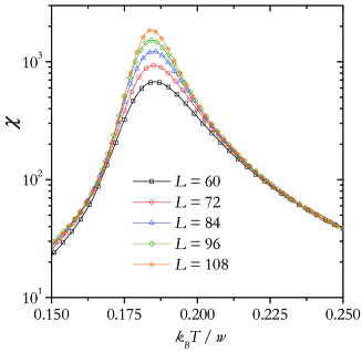
Figure 3: (Color online) Size dependence of the susceptibility as a function of temperature. The error in each measurement is smaller that the size of the symbols.

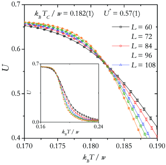
Figure 4: (Color online) $U$ versus $k_{B}T/w$, for different sizes. From their intersections one obtained $k_{B}T_{c}/w$. In the inset, the data are plotted over a wider range of temperatures.

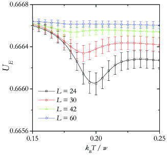
Figure 5: (Color online) Temperature variation of $U_{E}$ for various lattice sizes.

The conventional FSS implies the following behavior of $C$, $\langle\delta\rangle$, $\chi$ and $U$ at criticality,

$$C=L^{\alpha/\nu}\tilde{C}(L^{1/\nu}\epsilon)$$ (10)

$$\langle\delta\rangle=L^{-\beta/\nu}\tilde{\delta}(L^{1/\nu}\epsilon)$$ (11)

$$\chi=L^{\gamma/\nu}\tilde{\chi}(L^{1/\nu}\epsilon)$$ (12)

$$U=\tilde{U}(L^{1/\nu}\epsilon)$$ (13)

for $L\rightarrow\infty$, $\epsilon\rightarrow 0$ such that $L^{1/\nu}\epsilon$= finite, where ($\epsilon\equiv T/T_{c}-1$). Here $\alpha$, $\beta$, $\gamma$ and $\nu$ are the standard critical exponents of the specific heat ( $C\sim|\epsilon|^{-\alpha}$ for $\epsilon\rightarrow 0$, $L\rightarrow\infty$), order parameter ($\langle\delta\rangle\sim-\epsilon^{\beta}$ for $\epsilon\rightarrow 0^{-}$, $L\rightarrow\infty$), susceptibility($\chi\sim|\epsilon|^{\gamma}$ for $\epsilon\rightarrow 0$, $L\rightarrow\infty$) and correlation length $\xi$ ($\xi\sim|\epsilon|^{-\nu}$ for $\epsilon\rightarrow 0,L\rightarrow\infty$), respectively. $\tilde{C},\tilde{\delta},\tilde{\chi}$ and $\tilde{U}$ are scaling functions for the respective quantities. In the case of extended FSS,  GARTENHAUS ; CAMPBELL $\epsilon$ and $L$ in eqs. (10-13) are replaced by $\sigma\equiv 1-T_{c}/T$ and $L\sqrt{T}$, respectively.

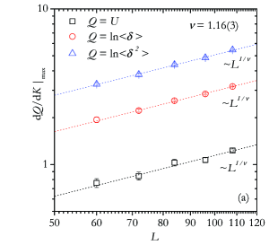
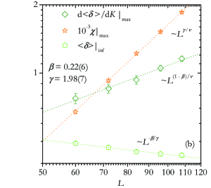
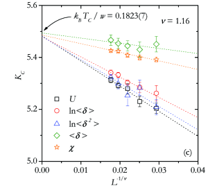
Figure 6: (Color online) (a) Log-log plot of the size dependence of the maximum values of derivatives of various thermodynamic quantities used to determine $\nu$. (b) Log-log plot of the size dependence of the maximum value of the susceptibility, the point of inflection of the order parameter and the maximum value of the derivative of the order parameter used to determine $\gamma$ and $\beta$, respectively. (c) $K_{c}(L)$ vs. $L^{-1/\nu}$ from several quantities as indicated. From extrapolation one obtains the estimation of the critical temperature. In all cases, dotted lines correspond to linear fits of the data and $L=60,72,84,96,108$.

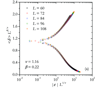
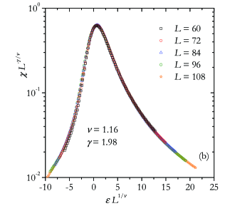
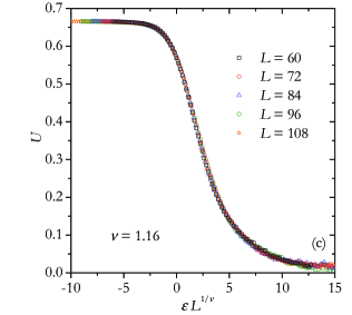
Figure 7: (Color online) Conventional data collapsing for: (a) the curves in Fig. 2; (b) the curves in Fig. 3; and (c) the curves in Fig. 4.

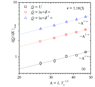
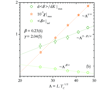
Figure 8: (Color online) Same as Fig. 6 for the extended scaling scheme.

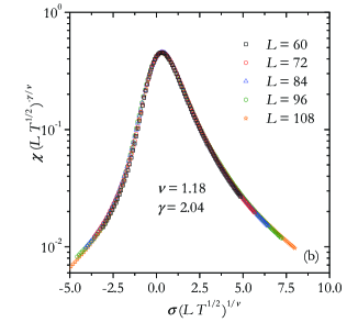
Figure 9: (Color online) Same as Fig. 7 for the extended scaling scheme.

We start with the calculation of the order parameter (Fig. 2), susceptibility (Fig. 3) and cumulant (Fig. 4) plotted versus $k_{B}T/w$ for several lattice sizes. Due to computational limitations, foot2 the curves in Fig. 2 do not clearly show the existence, at thermodynamic limit, of a finite temperature below which the order parameter is different from zero. In order to clarify this point, the inset in Fig. 2 shows the dependence of $\langle\delta\rangle$ on $L^{-1}$ for constant $T$. As it can be observed, $\langle\delta\rangle$ tends to a finite value (zero) for $T<T_{c}$ ($T>T_{c}$).

From the intersections of the curves in Fig. 4 one gets the estimation of the critical temperature. In this case, $k_{B}T_{c}/w=0.182(1)$, which is in good agreement with the value previously reported in the literature SURFSCI3 . In Ref. SURFSCI3, , the critical temperature was obtained from the peaks of the curves of the specific heat versus temperature (at fixed coverage) and coverage (at fixed temperature). A more rigorous study was not possible due to the lack of an adequate order parameter. In the inset, the data are plotted over a wider range of temperatures, exhibiting the typical behavior of the cumulants in presence of a continuous phase transition. With respect to the value of the cumulant at the transition temperature, $U^{*}$, this quantity was calculated by plotting $U^{*}(L)$ vs $L^{-1/\nu}$  Ferren , where the value of $U^{*}(L)$ was obtained by fixing $K$($\equiv w/k_{B}T$) at our estimate for $K_{c}$($\equiv w/k_{B}T_{c}$) and looking at the cumulant there (this is not shown here for brevity). In the thermodynamic limit we obtained $U^{*}=0.57(1)$. This value is consistent with the cumulant crossings shown in Fig. 4.

In order to discard the possibility that the phase transition is a first-order one, the energy cumulants [Eq. (9)] have been measured. As it is well-known, the finite-size analysis of $U_{E}$ is a simple and direct way to determine the order of a phase transition Binder2 ; Challa ; Vilmayr . Fig. 5 illustrates the energy cumulants plotted versus $k_{B}T/w$ for different lattice sizes ranging between $L=24$ and $L=60$. The values of the parameters used in the MC runs were $m=21$, $n_{1}=10^{5}$, $n_{2}=10^{5}$, $n_{MCS}=3\times 10^{5}$, $T_{1}=0.25$ and $T_{m}=0.15$. As it is observed, $U_{E}$ has the characteristic behavior of a continuous phase transition: the minima in the cumulants tend to $2/3$ as the lattice size is increased. This indicates that the latent heat is zero in the thermodynamic limit, which reinforces the arguments given in the paragraphs above.

Next, the critical exponents will be calculated. As stated in Refs. Ferren, ; Janke, ; Bin, , the critical exponent $\nu$ can be obtained by considering the scaling behavior of certain thermodynamic derivatives with respect to the inverse temperature $K$, for example, the derivative of the cumulant and the logarithmic derivatives of $\langle\delta\rangle$ and $\langle\delta^{2}\rangle$. In Fig. 6(a) we plot the maximum value of these derivatives as a function of system size on a log-log scale foot3 . The results for $1/\nu$ from these fits are given in the figure. Combining these three estimates we obtain $\nu=1.16(3)$ (see Table II). Once we know $\nu$, the critical exponent $\gamma$ can be determined by scaling the maximum value of the susceptibility Ferren ; Janke . Our data for $\chi|_{\rm max}$ are shown in Fig. 6(b). The value obtained for $\gamma$ is indicated in the figure and listed in Table II.

On the other hand, the standard way to extract the exponent ratio $\beta/\nu$ is to study the scaling behavior of $\langle\delta\rangle$ at the point of inflection, i. e., at the point where $d\langle\delta\rangle/dK$ is maximal. Since these points should scale as usual, $\left(K^{\langle\delta\rangle}_{\rm inf}-K_{c}\right)L^{1/\nu}\equiv\epsilon L^{1/\nu}={\rm const}$, we expect Janke

$${\langle\delta\rangle|}_{\rm inf}=L^{-\beta/\nu}\tilde{\delta}(\epsilon L^{1/\nu})\propto L^{-\beta/\nu},$$ (14)

where ${\langle\delta\rangle|}_{\rm inf}$ is the value of $\langle\delta\rangle$ at the point of inflection. In addition, since the derivative with respect to $K$ picks up a factor $L^{1/\nu}$ from the argument of the scaling function $\tilde{\delta}$,

$$\left.\frac{d\langle\delta\rangle}{dK}\right|_{\rm max}=L^{\left(-\beta/\nu+1/\nu\right)}\tilde{\delta}^{\prime}(\epsilon L^{1/\nu})\propto L^{\left(1-\beta\right)/\nu}.$$ (15)

The scaling of ${\langle\delta\rangle|}_{\rm inf}$ is shown in Fig. 6(b). The linear fit through all data points gives $\beta^{\left({\langle\delta\rangle|}_{\rm inf}\right)}=0.24(6)$. In the case of $d\langle\delta\rangle/dK|_{\rm max}$ [see Fig. 6(b)], the value obtained from the fit is $\beta^{\left(d\langle\delta\rangle/dK|_{\rm max}\right)}=0.20(8)$. Combining the two estimates, we obtain the final value $\beta=0.22(6)$, which is indicated in the figure and listed in Table II.

The finite-size scaling theory Binder0 ; Privman ; Privman1 ; Ferren allows for various efficient routes to estimate $T_{c}$ from MC data. One of this method, which was used in Fig. 4, is from the temperature dependence of $U(T)$ for different lattice sizes. An independent procedure to determine $T_{c}$ will be used in the following analysis. The method relies on the extrapolation of the positions $K_{c}(L)$ of the maxima of various thermodynamic quantities, which scale with system size like Binder0 ; Privman ; Privman1 ; Ferren

$$K_{c}(L)=K_{c}(\infty)+{\rm const}.L^{-1/\nu}.$$ (16)

Fig. 6(c) shows a plot of $K_{c}(L)$ vs. $L^{-1/\nu}$ for the maxima of the slopes of $\langle\delta\rangle$, $\left(d\langle\delta\rangle/dK\right)_{\rm max}$; $U$, $\left(dU/dK\right)_{\rm max}$; $\ln\langle\delta\rangle$, $\left(d\ln\langle\delta\rangle/dK\right)_{\rm max}$; $\ln\langle\delta^{2}\rangle$, $\left(d\ln\langle\delta^{2}\rangle/dK\right)_{\rm max}$, as well as of the susceptibility, $\chi_{\rm max}$. The lines are fits of the data to Eq. (16) with $\nu=1.16$. From extrapolation one obtains $K^{(A)}_{c}(\infty)$ [or $k_{B}T^{(A)}_{c}(\infty)/w$] for the different observables $A$. In this case, $k_{B}T^{(U)}_{c}(\infty)/w=0.1824(12)$; $k_{B}T^{(\ln\langle\delta\rangle)}_{c}(\infty)/w=0.1825(14)$; $k_{B}T^{(\ln\langle\delta^{2}\rangle)}_{c}(\infty)/w=0.1825(16)$; $k_{B}T^{(\langle\delta\rangle)}_{c}(\infty)/w=0.1820(20)$; and $k_{B}T^{(\chi)}_{c}(\infty)/w=0.1823(5)$. Combining these estimates we find a final value $k_{B}T_{c}/w=0.1823(7)$, which coincides, within numerical errors, with the value calculated from the crossing of the cumulants.

Strong corrections to scaling were observed to be present at small lattices and we excluded $L<60$ data from the calculations. On the other hand, the $L\geq 60$ data are not good enough to include corrections to scaling in the estimation of the critical exponents and critical temperature. Thus, the quoted errors in our results do not include systematic errors due to corrections to scaling that possibly could affect our data.

The scaling behavior can be further tested by plotting $\langle\delta\rangle L^{\beta/\nu}$ vs $|\epsilon|L^{1/\nu}$, $\chi L^{-\gamma/\nu}$ vs $\epsilon L^{1/\nu}$ and $U$ vs $|\epsilon|L^{1/\nu}$ and looking for data collapsing. Using our best estimates $k_{B}T_{c}/w=0.182$, $\nu=1.16$, $\beta=0.22$ and $\gamma=1.98$, we obtain very satisfactory scaling as it is shown in Fig. 7. This study leads to independent controls and consistency checks of the values of all the critical exponents. The collapses in Fig. 7 were calculated by following a conventional FSS scheme.

In the next, the analysis of Figs. 6 and 7 is repeated, this time applying the extended FSS scheme mentioned before. As it is shown in Fig. 8, the values obtained for the critical temperature $k_{B}T_{c}/w=0.1822(7)$ and the critical exponents $\nu=0.18(3)$, $\beta=0.23(6)$ and $\gamma=2.04(5)$ (see Table II) are in excellent agreement with those calculated using the conventional FSS. In addition, we apply the extended FSS scheme to collapse the data by plotting $U$, $\langle\delta\rangle$ and $\chi$ in terms of the variables $\sigma\equiv 1-T_{c}/T$ and $L\sqrt{T}$. The results are shown in Fig. 9. The behavior of the critical quantities for the extended FSS scheme is consistent with the behavior observed by following the conventional FSS scheme, which reinforces the robustness of the scaling analysis introduced here.

The critical exponents obtained by conventional and extended FSS, along with the fixed point value of the cumulants, $U^{*}=0.57(1)$, obtained in Fig. 4, suggest that the phase transition occurring for repulsive dimers on square lattices at $2/3$ monolayer coverage belongs to a new universality class. We say “suggest” because the lattice sizes studied here do not allow us to exclude a more complex critical behavior, for example, the presence of a tricritical point BORO5 ; WILDING1 ; WILDING2 . In order to elucidate this point, future studies on the whole phase diagram, including variables as coverage and an external field (coupled to the order parameter) breaking the orientational geometry of the phase, will be carried out.

Table 2: Critical exponents obtained from the fits shown in Figs. 6 and 8.

exponent	conventional	extended
	FSS	FSS
$\nu$	$1.16(3)$	$1.18(3)$
$\beta$	$0.22(6)$	$0.23(6)$
$\gamma$	$1.98(7)$	$2.04(5)$
$\alpha$	$\cdots$	$\cdots$

Finally, we will briefly refer to the specific heat exponent $\alpha$. The “roughness” of the curves of $C$ prevents a direct determination of $\alpha$. However, the usual hyperscaling relations inequalities of Rushbrooke, $\alpha+2\beta+\gamma\geq 2$, and Josephson, $d\nu+\alpha\geq 2$ (being $d$ the dimension of the space), predict a negative specific heat exponent $\alpha\approx-0.3$. This finding is consistent with the preliminary results obtained in the present study. Namely, even though the fluctuations in the energy are of the order of the statistical errors in the simulation results (reason for which the data are not shown here), it is possible to observe that the maxima of the curves of the specific heat remain practically constant as $L$ is increased. In other words, the specific heat seems not to diverge on approaching the transition. However, the present data do not allow us to be conclusive on this point and more work is needed to clearly elucidate the specific heats behavior of the model.

In summary, we have addressed the critical properties of repulsive dimers on two-dimensional square lattices at $2/3$ coverage. The results were obtained by using exchange MC simulations and FSS theory. The choice of an adequate order parameter [as defined in Eq. (2)] along with the exhaustive study of FSS presented here allow us $1)$ to confirm previous results in the literature, Phares ; SURFSCI3 namely, the existence of a continuous phase transition at $2/3$ coverage; $2)$ to calculate the critical temperature characterizing this transition; and $3)$ to obtain the complete set of static critical exponents for the reported transition. Though it is not possible to exclude the existence of a more complex critical behavior, the results suggest that the phase transition belongs to a new universality class.

- (1) H. E. Stanley, Introduction to Phase Transitions and Critical Phenomena (Oxford University Press, New York, 1971).
- (2) M. E. Fisher, Critical Phenomena (Academic Press, London, 1971).
- (3) K. Kawasaki, Phase Transitions and Critical Phenomena, edited by C. Domb and M. S. Green (Academic Press, London, 1972), Vol. 2, pag. 443.
- (4) R. J. Baxter, Exactly solved models in statistical mechanic (Academic Press, London, 1982).
- (5) J. M. Yeomans, Statistical Mechanics of Phase Transitions (Clarendon Press, Oxford, 1992).
- (6) N. Goldenfeld, Lectures on Phase Transitions and the Renormalization Group (Addison-Wesley, Reading, MA, 1992).
- (7) Phase Transitions and Critical Phenomena, edited by C. Domb and J. L. Lebowitz (Academic Press, London, 2001), Vol. 19.
- (8) T. L. Hill, J. Chem. Phys. 17, 520 (1949).
- (9) Phase Transitions in Surface Films, edited by J. G. Dash and J. Ruvalds (Plenum, New York, 1980).
- (10) Phase Transitions in Surface Films 2, edited by H. Taub, G. Torso, H. J. Lauter, and S. C. Fain, Jr. (Plenum, New York, 1991).
- (11) G. A. Somorjai and M. A. Van Hove, Adsorbed Monolayers on Solid Surfaces (Springer-Verlag, New York, 1979).
- (12) M. Schick, J. S. Walker and M. Wortis, Phys. Rev. B 16, 2205 (1977).
- (13) K. Binder, Applications of the Monte Carlo Method in Statistical Physics. Topics in Current Physics (Springer, Berlin, 1984), Vol. 36.
- (14) K. Binder and D. P. Landau, Phys. Rev. B 21, 1941 (1980).
- (15) D. P. Landau, Phys. Rev. B 27, 5604 (1983).
- (16) K. Binder and D. P. Landau, Phys. Rev. B 30, 1477 (1984).
- (17) D. P. Landau and K. Binder, Phys. Rev. B 31, 5946 (1985).
- (18) D. P. Landau and K. Binder, Phys. Rev. B 41, 4633 (1990).
- (19) E. Domany, M. Schick, J. S. Walker, and R. B. Griffiths, Phys. Rev. B 18, 2209 (1978).
- (20) E. Domany and M. Schick, Phys. Rev. B 20, 3828 (1979).
- (21) M. Schick, Prog. Surf. Sci. 11, 245 (1981).
- (22) A. Patrykiejew, S. Sokolowski, and K. Binder,Surf. Sci. Rep. 37, 207 (2000).
- (23) A. J. Phares, F. J. Wunderlich, J. D Curley, and D. W. Grumbine, Jr., J. Phys. A: Math. Gen. 26, 6847 (1993).
- (24) A. J. Ramirez-Pastor, J. L. Riccardo, and V. D. Pereyra, Surf. Sci. 411, 294 (1998).
- (25) A. J. Ramirez-Pastor, J. L. Riccardo, and V. D. Pereyra, Langmuir 16, 10167 (2000).
- (26) M. S. Nazzarro, A. J. Ramirez-Pastor, J. L. Riccardo, and V. D. Pereyra, Surf. Sci. 391, 267 (1997).
- (27) F. Romá, A. J. Ramirez-Pastor, and J. L. Riccardo, Langmuir 16, 9406 (2000).
- (28) F. Romá, A. J. Ramirez-Pastor, and J. L. Riccardo, Phys. Rev. B 68, 205407 (2003).
- (29) F. Romá, A. J. Ramirez-Pastor, and J. L. Riccardo, Phys. Rev. B 72, 035444 (2005).
- (30) P. M. Pasinetti, F. Romá, J. L. Riccardo and A. J. Ramirez-Pastor, Phys. Rev. B 74, 155418 (2006).
- (31) M. Borówko and W. Rżysko, J. Colloid Interface Sci. 244, 1 (2001).
- (32) W. Rżysko and M. Borówko, J. Chem. Phys. 117, 4526 (2002).
- (33) W. Rżysko and M. Borówko, Surf. Sci. 520, 151 (2002).
- (34) W. Rżysko and M. Borówko, Surf. Sci. 600, 890 (2006).
- (35) W. Rżysko and M. Borówko, Phys. Rev. B 67, 045403 (2003).
- (36) V. Privman, Finite Size Scaling and Numerical Simulation of Statistical Systems (World Scientific, Singapore, 1990).
- (37) V. Privman, P. C. Hohenberg, and A. Aharony, Phase Transitions and Critical Phenomena, edited by C. Domb and J. L. Lebowitz (Academic Press, New York, 1991), Vol. 14.
- (38) S. Gartenhaus and W. S. McCullough, Phys. Rev. B 38, 11688 (1988).
- (39) I. A. Campbell, K. Hukushima, and H. Takayama, Phys. Rev. Lett. 97, 117202 (2006).
- (40) As in the case of the ordered phase occurring for linear -mers on square lattices at monolayer coverage, PRB5 the phase transition at monolayer coverage is accomplished by a breaking of the translational and orientational symmetries.
- (41) K. Hukushima and K. Nemoto, J. Phys. Soc. Jpn. 65, 1604 (1996).
- (42) D. J. Earl and M. W. Deem, Phys. Chem. Chem. Phys. 7, 3910 (2005).
- (43) N. Metropolis, A.W. Rosenbluth, M.N. Rosenbluth, A.H. Teller and E. Teller, J. Chem. Phys. 21, 1087 (1953).
- (44) H. G. Katzgraber, M. Körner, and A. P. Young, Phys. Rev. B 73, 224432 (2006).
- (45) As it is well-known, MC simulations of -mers at equilibrium are very time consuming. Consequently, the finite-size scaling study was carried out for lattice sizes up to , with an effort reaching almost the limits of our computational capabilities.
- (46) M. S. S. Challa, D. P. Landau and K. Binder, Phys. Rev. B 34, 1841 (1986).
- (47) K. Vollmayr, J. D. Reger, M. Scheucher and K. Binder, Z. Phys. B: Condens. Matter 91, 113 (1993).
- (48) A. M. Ferrenberg and D. P. Landau, Phys. Rev. B 44, 5081 (1991).
- (49) W. Janke, M. Katoot and R. Villanova, Phys. Rev. B 49, 9644 (1994).
- (50) K. Binder and E. Luijten, Physics Reports 344, 179 (2001).
- (51) In this paper, the temperature derivatives were taken by averaging the slopes of two adjacent data points as follows: . Error bars were estimated by propagation of errors from the last equation. On the other hand, the coordinates of each maximum were calculated by fittting a three-order polynomial to a set of between 15 and 20 data points around this critical value. Polynomials of order 2 and 4 were also used as fitting functions and the results did not change significantly.
- (52) N. B. Wilding, and P. Nielaba, Phys. Rev. E 53, 926 (1996).
- (53) N. B. Wilding, F. Schmid, and P. Nielaba, Phys. Rev. E 58, 2201 (1998).