Long-Range Effects in Layered Spin Structures

Abstract

We study theoretically layered spin systems where long-range dipolar interactions play a relevant role. By choosing a specific sample shape, we are able to reduce the complex Hamiltonian of the system to that of a much simpler coupled rotator model with short-range and mean-field interactions. This latter model has been studied in the past because of its interesting dynamical and statistical properties related to exotic features of long-range interactions. It is suggested that experiments could be conducted such that within a specific temperature range the presence of long-range interactions crucially affect the behavior of the system.

Many of the forces that we see in the universe have a long-range nature where in $d$ dimensions a pairwise interaction potential decays as $V(r)\sim 1/r^{d+s}$ with $-d\leq s\leq 0$. Examples include gravitational interactions, Coulomb and magnetic forces. Nowadays there is a vast literature which describes various exotic nonlinear and statistical properties of many-body systems with long-range interactions such as disagreement of predictions of microcanonical and canonical ensembles, negative specific heat and temperature jumps, etc. ruffobook . However, most of these studies are purely theoretical and there have been only few suggestions on how to test experimentally all these peculiarities. One example is the astrophysical observation of negative specific heat astro which is an outcome of the truly long range nature of the gravitational force. In addition, it has been suggested that systems composed of a small number of particles can show negative specific heat part due to non-additivity even when the interaction is short range. This has been verified experimentally in nuclear collisions nuclear , atomic sodium clusters sodium and in molecular clusters cluster . However no experimental test of these predictions has been carried out for a laboratory system with long range interactions.

Figure 1: Left graph: schematic arrangement of spin $s=1/2$ $Cu^{+2}$ ions in a $(C_{\nu}H_{2\nu+1}NH_{3})_{2}CuCl_{4}$ layered compound. Right graph: Suggested form of the sample which allows the observation of the spontaneous flips of the magnetization vector (thick arrows at the middle) which are predicted by Hamiltonian (7) to which the microscopic model (1) effectively reduces.

This Letter aims at proposing testable effects of dipolar magnetic forces, whose long-range nature is a consequence of the cubic decay law of the potential $V(r)\sim 1/r^{3}$ . This law results in a strong dependence of the dipolar energy on the sample shape (see e.g. Ref. landau ). However, in ordinary magnetic systems, dipolar energy is about a thousand times smaller than Heisenberg exchange interactions between nearby spins. Therefore, in most cases the role of long-range forces is to introduce some anisotropy which determines the ordering direction in the magnetic sample. On the other hand, in nuclear magnets, where magnetic order is fully defined by dipolar interaction, one has to go down to nano Kelvin temperatures to observe ordering oja .

In this Letter, we propose to examine more closely magnetic layered spin structures (e.g. $(C_{\nu}H_{2\nu+1}NH_{3})_{2}CuCl_{4}$ sievers ) in which the effective magnetic interaction between electronic spins is predominantly dipolar. In particular, we examine rod shaped layered spin structures, whose microscopic Hamiltonian can be effectively reduced to that of a one dimensional coupled rotator model with both nearest neighbor coupling and a dominant mean-field interaction term resulting from the dipolar forces. We suggest that these compounds provide a system in which exotic phenomena that characterize coupled rotator models with both short and long-range couplings campa ; mukruf could readily be observed. Here, we propose to verify experimentally the presence of all-to-all mean-field couplings by monitoring the time-scales of spontaneous magnetization flips below the magnetic transition. Similar effects of magnetization reversals could in principle take place in systems with only short-range interactions ising . However, here we propose to explore the experimental conditions in which collective reversals are driven by the presence of long-range interactions, and therefore their existence becomes strongly dependent on the shape of the sample. Moreover, the average reversal time is expected to grow as the exponential of the volume of the sample as opposed to the case of short range interactions where it grows only as the exponential of the surface area ising . In addition, magnetization reversals due to long range interactions are expected to be sharper, since they involve at once the entire sample.

The magnetic arrangement of the class of compounds $(C_{\nu}H_{2\nu+1}NH_{3})_{2}CuCl_{4}$ is schematically given in Fig. 1 (see for more details Refs. dupas ; miedema ). The system is composed of ferromagnetic layers with strong intralayer interactions, $W$, and a weak coupling, $w$, between the layers which is either ferromagnetic for $\nu=1$ or antiferromagnetic for $\nu>1$. This allows us to consider the three-dimensional spin system at temperatures or energies well below $W$ as a quasi-one dimensional ferromagnetic or anti-ferromagnetic spin chain consisting of classical spins, with each spin in the chain representing a whole layer. The forces in the system are provided by the exchange interactions between the effective spins in the chain (short-range forces) and the dipolar interactions among all spins (long-range forces). The interlayer exchange interaction turns out to be comparable with the dipolar interactions making these systems excellent candidates for considering long-range effects, even in the case of a small number of layers. Note that, as expected, the shape of the sample is rather important in systems with dipolar interactions. A particularly interesting case is that of ferromagnetic interlayer coupling ($\nu=1$) with a sample shape for which dipolar forces favor ferromagnetic ordering such as in a rod cut along the layer planes (rod along axis $z$ in Fig. 1). This case will be discussed in detail below.

These systems have been modelled previously including only the anisotropic contribution of the dipolar forces (see e.g. Ref. dupas ) while the long-range character of these forces was neglected. At this stage we include fully the dipolar interactions and the Hamiltonian reads

$${\cal H}=-W\sum\limits_{I,<i,j>}\left(s_{Ii}^{z}s_{Ij}^{z}+\eta s_{Ii}^{y}s_{Ij}^{y}+\xi s_{Ii}^{x}s_{Ij}^{x}\right)-w\sum\limits_{I,<i,j>}\vec{s}_{Ii}\vec{s}_{I+1,j}+\sum\limits_{Ii\neq Jj}\frac{2\mu_{B}^{2}}{r^{3}}\left(\vec{s}_{Ii}\vec{s}_{Jj}-3\frac{(\vec{s}_{Ii}\vec{r})(\vec{s}_{Jj}\vec{r})}{r^{2}}\right)$$ (1)

where the first sum represents the intralayer exchange interaction (indices $i$ and $j$ refer to nearest neighbor spins within the same layer, while the indices $I$ and $J$ number the layers), $\mu_{B}$ is Bohr’s magneton and $\vec{r}$ is the vector between the sites of the spins $\vec{s}_{Ii}$ and $\vec{s}_{Jj}$. The parameters $\xi$ and $\eta$ ($<1$) yield biaxial hard axes anisotropies along the $x$ and $y$ axes, respectively. They are a result of the crystallographic forces and take into account out-of plane and in-plane anisotropies (note that the main contribution to the in-plane anisotropy comes from dipolar forces themselves, see below). The second sum stands for the interlayer exchange interactions (with $i$ and $j$ now referring to nearest neighbor spins in adjacent layers) and the last term describes dipolar interactions among all spins. According to dupas ; miedema $W\simeq 10^{4}w$ in the compounds $(C_{1}H_{3}NH_{3})_{2}CuCl_{4}$. At low temperatures all spins in a single layer are ordered ferromagnetically and therefore the spin vector $\vec{s}_{Ii}$ could be considered as independent of the index $i$, $\vec{s}_{I}\equiv\vec{s}_{Ii}$, and this represents the spin of a whole layer. This is justified only if one works below the ordering temperature of a single layer, which approximately coincides with the intralayer exchange constant $W$. Under the additional condition $nw<W$ ($n$ is the number of spins in a single layer), in a certain temperature range each layer will be ordered ferromagnetically, while the transition to 3D ordering will be strongly affected by the existence of long-range dipolar forces (which are comparable with the short range interlayer exchange $w$). We consider the thermodynamic properties of the system under such conditions. Applying the ordinary procedure to calculate the dipolar sum, one can divide it into a short-range contribution (restricting ourselves to consider the interaction between nearest neighbors) and a long-range one landau . Then (1) can be rewritten in the following one-dimensional representation (see Ref. sieversprb )

$${\cal H}=n\left[B_{x}\sum\limits_{J=1}^{N}\bigl{(}s_{J}^{x}\bigr{)}^{2}+B_{y}\sum\limits_{J=1}^{N}\bigl{(}s_{J}^{y}\bigr{)}^{2}-2\omega_{ex}\sum\limits_{J=1}^{N-1}\bigl{(}s_{J}^{y}s_{J+1}^{y}+s_{J}^{z}s_{J+1}^{z}\bigr{)}-\frac{\omega_{M}}{N}\Bigl{(}\sum\limits_{J=1}^{N}s_{J}^{z}\Bigr{)}^{2}+\frac{\omega_{M}}{2N}\Bigl{(}\sum\limits_{J=1}^{N}s_{J}^{y}\Bigr{)}^{2}\right],$$ (2)

where $B_{x}=4W(1-\xi)$ and $B_{y}=4W(1-\eta)$ define the hard axis anisotropies along $x$ and $y$, respectively (the out-of plane anisotropy being much larger than the in-plane one $B_{x}\gg B_{y}$), $N$ is the number of layers, $\omega_{ex}$ is an effective exchange constant between the layers consisting of the sum of the exchange constant $w$ between the neighboring spins of the different layers and the contribution of dipolar forces between the same spins. Thus

$$\omega_{ex}=2w-\frac{2\mu_{B}^{2}}{r_{a}^{3}}\left(2-\frac{3q_{a}^{2}}{r_{a}^{2}}\right),$$ (3)

Where $q_{a}$ and $r_{a}$ are the distances between nearest neighboring spins within the same layers and different layers, respectively. In the case of the considered compound $q_{a}=5.25\cdot 10^{-8}$cm and $r_{a}=9.97\cdot 10^{-8}$cm miedema . Finally the last two mean-field terms come from the long-range part of dipolar forces. Moreover, $\omega_{M}=(4\pi/3)(2\mu_{B}^{2}/v_{0})$ and $v_{0}$ is the volume of the unit cell of the lattice. Note that the nearest neighbor part of dipolar forces favors antiferromagnetic ordering of the spins in neighboring layers, while the long-range component of the forces is ferromagnetic along $z$. The measured value for the out-of plane anisotropy is $B_{x}=240$mK, while the in-plane anisotropy constant $B_{y}$ is less than $5$mK. The exchange constants is $\omega_{ex}=4.8$mK (see e.g. Ref. dupas ), and $\omega_{M}=16$mK. Thus, we have:

$$B_{x}/\omega_{M}=15,\quad B_{y}/\omega_{M}\approx 0.2,\quad\omega_{ex}/\omega_{M}=0.3.$$ (4)

As is evident, the out-of plane anisotropic term is associated with a much larger energy scale than all the others and therefore we have neglected in (2) all the terms which include the $s_{x}$ component of the spins which emerge from dipolar or exchange interlayer forces.

We now consider the torque equation

$$\frac{d{\vec{s}_{J}}}{dt}={\vec{s}_{J}}\times{\vec{H}}_{J}~{},$$ (5)

where ${\vec{H}}_{J}=-{\partial{\cal H}}/{\partial{\vec{s}_{J}}}$ is an effective magnetic field acting on the spin $\vec{s}_{J}$. Noting that $|\vec{s}_{J}|=1/2$, it is natural to adopt the definitions $\vec{S}_{J}\equiv 2\vec{s}_{J}$, $S_{J}^{y}=\sqrt{1-(S_{J}^{x})^{2}}\sin\theta_{J}$ and $S_{J}^{z}=\sqrt{1-(S_{J}^{x})^{2}}\cos\theta_{J}$ which yield the equations of motion in terms of angular variable $\theta_{J}$ and of $S_{J}^{x}$. Observing that $B_{x}$ is the largest energy scale in the Hamiltonian , one can simplify the equations of motion for $S_{J}^{y}$ as follows

$$\frac{d\theta_{J}}{dt}=-nB_{x}S_{J}^{x}$$ (6)

and approximate $\sqrt{1-(S_{J}^{x})^{2}}\approx 1$. Then, substituting $S_{J}^{x}$ from the last equation into Hamiltonian (2), we obtain the following effective Hamiltonian, which includes only the angles $\theta_{J}$’s, and their time derivatives

$${\cal H^{\prime}}=\frac{2{\cal H}}{n\omega_{M}}=\frac{1}{2}\sum\limits_{J=1}^{N}\left[\frac{d\theta_{J}}{dt}\right]^{2}-\frac{\omega_{ex}}{\omega_{M}}\sum\limits_{J=1}^{N-1}\cos(\theta_{J+1}-\theta_{J})+\frac{B_{y}}{2\omega_{M}}\sum\limits_{J=1}^{N}\sin^{2}\theta_{J}-\frac{1}{2N}\Bigl{(}\sum\limits_{J=1}^{N}\cos\theta_{J}\Bigr{)}^{2}+\frac{1}{4N}\Bigl{(}\sum\limits_{J=1}^{N}\sin\theta_{J}\Bigr{)}^{2}~{},$$ (7)

where the dimensionless time is introduced via the transformation $t\rightarrow tn\sqrt{B_{x}\omega_{M}}$. The above model describes a system of coupled rotators with nearest neighbor and all-to-all mean-field interactions.

In analogy with the similar system considered in Ref. campa , we can derive the thermodynamic and dynamical properties of the model (7). It follows that, in the energy range $-0.3<\varepsilon<\varepsilon_{c}=0.376$, two maximal entropy states with opposite magnetization $m=(\sum\limits_{J=1}^{N}\cos\theta_{J})/N$ are present and, in principle, for finite $N$, the system can flip between these states. Above the critical energy $\varepsilon_{c}$ the system is characterized by a single maximum entropy state at $m=0$. At $\varepsilon_{c}$ a second order phase transition of the mean-field type is present. The lower energy limit derives from the fact that, in the thermodynamic limit ($N\rightarrow\infty$), the energy $\varepsilon$ satisfies the condition $\varepsilon>-m^{2}/2-\omega_{ex}/\omega_{M}$. It follows that below $\varepsilon=-{\omega_{ex}}/{\omega_{M}}\simeq-0.3$ there is an ergodicity breaking region mukruf , where the system retains its magnetization direction for infinitely long time. If the system energy is slightly above the ergodicity breaking limit, magnetization flips are very rare. Simulating the system using torque equation (5) does not reveal any flip for observable time scales, i.e. the system behaves like in the ergodicity breaking region.

Examining the dynamics of the one-dimensional spin chain (2) at $\varepsilon=0.2$, sufficiently above the ergodicity breaking region, the time evolution of the magnetization displays the expected behavior (see upper graph in Fig. 2). We then compute numerically the probability distribution function (PDF) of $m$, $P(m)$, and present the data of $(1/N)\log(P(m))$ as circles in the inset. These are compared (modulo a vertical normalization shift) with the analytical curve for the entropy derived for Hamiltonian (7). The agreement is impressively good, considering the numerous approximations we have made when deriving Hamiltonian (7) from (2).

If now one further increases the system energy above the critical one, $\varepsilon_{c}$, magnetization fluctuates around zero and the corresponding PDF is presented in the lower graph of Fig. 2, together with the analytical prediction, again in very good agreement.

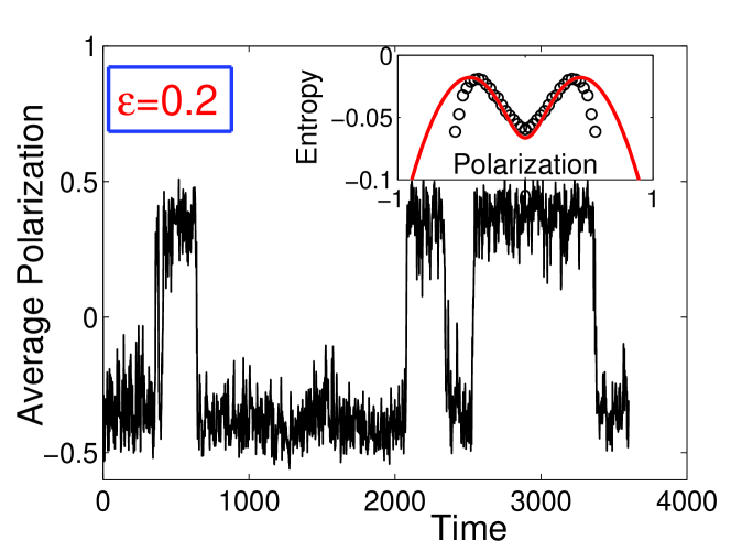
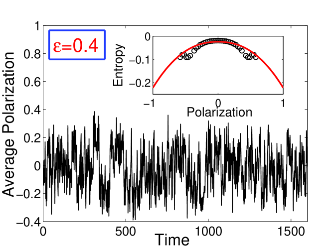
Figure 2: Main plots: Numerical simulations of the one dimensional spin chain model (2), (5) with different energies: $\varepsilon=0.2$ (upper graph) and $\varepsilon=0.4$ (lower graph), i.e. below and above the second order phase transition energy $\varepsilon_{c}=0.376$ predicted for Hamiltonian (7). The number of layers in the simulations is taken $N=100$. Insets show the corresponding entropy curves (solid lines) and data obtained from the PDF of the magnetization (open circles).

Let us conclude with a few remarks that are relevant for the experimental implementation. Let us recall that, throughout this paper, we have considered a rod shaped sample. Moreover, as stated above, the reduction of the Hamiltonian to a one-dimensional rotator model holds only if $nw<W$. Thus, for the compound under consideration, $n$ should be less than $10000$. Hence, in a real experiment, one should examine samples of typical size $n=20\times 500$ within a single layer and, e.g., $N=20$ layers in total. In contrast, in spherical samples with about the same number of spins per layer, long-range effects will be negligible and only short-range forces are left in the effective one-dimensional model: no phase transition will be present and, therefore, magnetization flips will be absent.

In summary, we have studied theoretically the layered spin structure $(C_{\nu}H_{2\nu+1}NH_{3})_{2}CuCl_{4}$ and showed that, under certain conditions, it could be modeled as a system of coupled rotators with both short and mean-field interactions. In experiments, this could be confirmed by the presence of magnetization flips for $\nu=1$ (ferromagnetic interlayer short-range interactions). When $\nu>1$ the short-range interlayer coupling is antiferromagnetic, while each layer is still ordered ferromagnetically. For an appropriate choice of the short versus long-range coupling (which could be precisely controlled by changing the length of rod shaped sample), the latter compounds could serve as a laboratory system for which various exotic phenomena, such as ensemble inequivalence, negative specific heat, temperature jumps, etc. campa ; new , characterizing systems with long-range interactions, could be observed.

We would like to thank A.J. Sievers for multiple useful suggestions and discussions. R. Kh. acknowledges support by Marie-Curie international incoming fellowship award (contract No MIF1-CT-2005-021328) and USA CRDF Award # GEP2-2848-TB-06. We also acknowledge financial support of the Israel Science Foundation (ISF) and of the PRIN05 grant on Dynamics and thermodynamics of systems with long-range interactions. We thank the Newton Institute in Cambridge (UK) for the kind hospitality during the programme “Principles of the Dynamics of Non-Equilibrium Systems” where part of this work was carried out.

References

- (1) T. Dauxois, S. Ruffo, E Arimondo, M. Wilkens, Dynamics and Thermodynamics of Systems with Long Range Interactions, Lecture Notes in Physics, v. 602, Springer (2002).
- (2) T. Padmanabhan, Phys. Reports, 188, 285 (1990).
- (3) R.M. Lynden-Bell, Mol. Phys. 86, 1353 (1995).
- (4) D’Agostino et al, Phys. Lett. B, 473, 219 (2000)
- (5) M. Schmidt et al. Phys. Rev. Lett. 86, 1191 (2001).
- (6) F. Gobet et al , Phys. Rev. Lett. 87, 203401 (2001).
- (7) L.D. Landau, E.M. Lifshits, Course of theoretical physics. v.8: Electrodynamics of continuous media, 1st edition, London, Pergamon, (1960).
- (8) A.S. Oja, O.V. Lounasmaa, Rev. Mod. Phys. 69, 1 (1997).
- (9) M. Sato, A.J. Sievers, Nature, 432, 486 (2004); J.P. Wrubel, M. Sato, A.J. Sievers, Phys. Rev. Lett., 95, 264101 (2005); M. Sato, A.J. Sievers, Phys. Rev. B, 71, 214306, (2005).
- (10) A. Campa, A. Giansanti, D. Mukamel, S. Ruffo, Physica A, 365, 120 (2006).
- (11) D. Mukamel, S. Ruffo, N. Schreiber, Phys. Rev. Lett., 95, 240604 (2005).
- (12) K. Brendel, G.T. Barkema, H. van Beijeren, Phys. Rev. E, 67, 026119 (2003).
- (13) A. Dupas, K. Le Dang, J.-P. Renard, P. Veillet, J. Phys. C: Solid State Phys., 10, 3399, (1977).
- (14) L.J. de Jongh, A.R. Miedema, Adv. Phys., 23, 1, (1974).
- (15) L. Q. English, M. Sato, and A. J. Sievers, Phys. Rev. B, 67, 024403 (2003).
- (16) P. de Buyl, D. Mukamel, S. Ruffo, AIP Conf. Proceedings, 800, 533 (2005).