Edge Transport in 2D Cold Atom Optical Lattices

Abstract

We theoretically study the observable response of edge currents in two dimensional cold atom optical lattices. As an example we use Gutzwiller mean-field theory to relate persistent edge currents surrounding a Mott insulator in a slowly rotating trapped Bose-Hubbard system to time of flight measurements. We briefly discuss an application, the detection of Chern number using edge currents of a topologically ordered optical lattice insulator.

The response theory of transport is a remarkably precise framework used to analyze the observable effects of applied potentials in a broad class of solid state systems. It is natural to ask how experiments on neutral cold atoms confined to optical lattices Oplat , predicted to hold a variety of novel phases of matter Lewenstein similar to those found in the solid state, can make contact with an equivalent quantitative framework. Recent experimental work on cold atom optical lattices demonstrates essential ingredients in establishing quantitative response: applied potentials and detection of conserved quantities. A primary tool for detection relies on time of flight (TOF) imaging which provided the first evidence for Bose-Einstein condensation Ketterle and revealed phases of optical lattice realizations of Bose-Hubbard (BH) models Jaksch ; Greiner ; Altman ; Bloch ; Spielman .

By combining TOF with externally applied potentials recent work has demonstrated transport in one dimensional optical lattices Pezze ; Porto . In a closed two dimensional system the notion of “transport” is less direct. A recent experiment has applied rotation to weak lattices Cornell confining bosons. While far from the single band BH limit, this experiment reveals vortex pinning arising from the weak lattice. Recent work magnetic ; Demler_FQHE also suggests that uniform effective magnetic fields (equivalent to rotation) may be applied to optical lattices already in the BH limit. Either implementation, rotation or an effective magnetic field, can be used as an applied potential valuable in establishing persistent currents, and therefore transport, in two dimensional lattices.

Concurrent with experimental progress, a variety of cold atom phases have been proposed in two dimensional optical lattices Lewenstein . Some of the proposed lattice models have rich phase diagrams with particularly intriguing or even unknown ground states, including: extended BH models Goral ; Lewenstein ; Scarola , higher band spin models Girvin , fractional quantum Hall models Demler_FQHE , and the Kitaev spin model Kitaev ; Demler_Spin ; Zoller . We ask how insulating phases arising in two dimensional lattice models can be studied using a combination of externally applied potentials and TOF.

Below we argue that trapping leads to edge states which serve as a probe of bulk insulating states. As a concrete and relevant example we study the slowly rotating BH model in detail. Other studies have considered vortex configurations in the superfluid phase of the rotating uniform BH model Wu ; Carr . Here we study edge effects in the Mott insulating phase of the slowly rotating trapped BH model. We propose that diamagnetic response of edge states can indeed be observed thereby offering a quantitative response probe of a variety of bulk two dimensional insulators. We briefly discuss implications for another insulator where edge states can be used to detect the Chern number Hatsugai ; Kitaev ; Qi of a topologically ordered insulator, the non-Abelian ground state of the Kitaev model.

We first note that response to externally applied fields can be obtained at a quantitative level by analyzing TOF measurements. TOF can be related to the momentum density, $\rho_{\bm{k}}$, of particles with lattice momentum ${\bm{k}}$ originally trapped in an optical lattice. Observation of $\rho_{\bm{k}}$ (with sufficient accuracy) can be combined with input parameters to restore quantities of the form: $\mathcal{J}\equiv\sum_{{\bm{k}}}\mathcal{W}_{\bm{k}}\rho_{\bm{k}},$ where $\mathcal{W}_{\bm{k}}$ is any function of ${\bm{k}}$ which can be accurately determined from input experimental parameters. By defining $\mathcal{W}_{\bm{k}}=\mathcal{M}_{\bm{k}}(\partial E_{\bm{k}}/\partial k_{\alpha})$ we obtain two examples: the free-particle number and energy currents in the direction $\alpha$ with the choices $\mathcal{M}_{\bm{k}}=1$ and $\mathcal{M}_{\bm{k}}=E_{\bm{k}}$, respectively. Here, $E_{\bm{k}}$ is the single particle energy determined by optical lattice parameters. As we will show, diamagnetic current flowing along sufficiently narrow edges of optical lattice insulators can be written in the form $\mathcal{J}$ allowing restoration of the edge current.

To study the observable response of insulating states in trapped optical lattices we consider the two-dimensional BH model on a square lattice in the presence of rotation (or, equivalently, an effective magnetic field magnetic ; Demler_FQHE ) as a first step in establishing quantitative response in systems nearest ongoing experiments. Using the Peierls substitution Peierls the BH model in the rotating frame is:

$$H = -t\sum_{\langle i,j\rangle}\left[\exp{(i\mathcal{A}_{i,j})}a_{i}^{\dagger}a_{j}^{\vphantom{\dagger}}+{\rm{h.c.}}\right]$$ (1)

$$+ \frac{U}{2}\sum_{i}n_{i}(n_{i}-1)-\sum_{i}\left(\mu-\tilde{\kappa}|{\bm{r}}_{i}|^{2}\right)n_{i},$$

where $a_{i}^{\dagger}$ and $n_{i}$ are the boson creation and number operators at the site $i$, respectively. The parameters include the hopping, $t$, the onsite interaction energy, $U$, and the chemical potential, $\mu$. The last term is due to the trapping potential which adds a site dependent chemical potential at the square lattice coordinate in the $xy$ plane, $\bm{r}_{i}=(i_{x},i_{y})$, parameterized by a modified trapping parameter $\tilde{\kappa}=\kappa-m(\Omega a)^{2}/2$, in units of the lattice spacing, $a$ (half the wavelength of the lasers defining the optical lattice). The trapping parameter is modified by a term due to rotation, with angular frequency, $\Omega$, of particles of mass $m$. In what follows we find that, for $\text{Rb}^{87}$ atoms with $\mu/U=0.4$, $U/E_{R}\sim 0.1$, and $\kappa/U=1.2\times 10^{-3}$ the modification is negligible for the rotation frequencies studied here giving $\tilde{\kappa}\approx\kappa$. $E_{R}=h^{2}/(8ma^{2})$ is the recoil energy. The rotation also modifies the hopping term to give a phase: $\mathcal{A}_{i,j}=(\pi^{2}\hbar\Omega/2E_{R})\int_{i}^{j}(\hat{z}\times{\bm{r}})\cdot d{\bm{s}},$ which can be thought of as an integral over a vector potential due to an effective magnetic field, $B^{*}\hat{z}$, acting on an effective charge $q^{*}$ such that $q^{*}B^{*}=2m\Omega$. In the rotating frame the neutral bosons experience an effective magnetic field which induces a persistent current opposing the applied effective field.

In the linear response regime, $\hbar\Omega/E_{R}\ll 1,$ we can define Scalapino a number current in the direction $\alpha$ in response to the static applied potential, $\mathcal{A}$: $J_{i,\alpha}=it\hbar^{-1}\left(a_{i}^{\dagger}a_{i_{\alpha}}^{\vphantom{\dagger}}-{\rm{h.c.}}\right)-\hbar^{-1}\mathcal{A}_{i,i_{\alpha}}K_{i,i_{\alpha}}$ where the first term is the paramagnetic number current and the second term is the diamagnetic number current which contains the kinetic term: $K_{i,i_{\alpha}}\equiv t\left(a_{i}^{\dagger}a_{i_{\alpha}}^{\vphantom{\dagger}}+{\rm{h.c.}}\right).$ The total diamagnetic number current is an observable response to our externally applied field giving: $J^{\rm D}_{\alpha}=-\hbar^{-1}\sum_{l}K_{i,i_{\alpha}}\mathcal{A}_{i,i_{\alpha}}.$ In general $J^{\rm D}$ cannot be written in the form $\mathcal{J}$ and it is therefore not clear how we can relate such a quantity to TOF measurements. In what follows we will show that when the diamagnetic current is confined to the edge of the system (and therefore $\mathcal{A}$ varies sufficiently slowly) we can write an approximation to $J^{\rm D}$ which in turn can be related to TOF. Consider the following approximation: $\bar{J}^{\rm D}_{\alpha}\equiv-\hbar^{-1}\mathcal{A}_{i^{e},i^{e}_{\alpha}}\sum_{i}K_{i,i_{\alpha}},$ where: $\mathcal{A}_{i^{e},i^{e}_{\theta}}=(\pi^{2}\hbar\Omega/2E_{R})(\hat{z}\times{\bm{r}}_{i^{e}})\cdot\hat{\theta}.$ Here ${\bm{r}}_{i^{e}}$ indicates the average position of the edge superfluid order parameter, $\psi_{i}=\langle a^{\dagger}_{i}\rangle,$ giving $\hat{r}\cdot{\bm{r}}_{i^{e}}=(\sum_{i}|\psi_{i}|^{2}\hat{r}\cdot{\bm{r}}_{i})/(\sum_{i}|\psi_{i}|^{2}).$ By Fourier transforming and taking the expectation value with respect to the ground state we find: $\langle\bar{J}^{\rm D}_{\theta}\rangle=-2t\mathcal{A}_{i^{e},i^{e}_{\theta}}(\hbar Z)^{-1}\sum_{{\bm{k}},{\bm{\delta}}}\rho_{{\bm{k}}}\cos\left({\bm{k}}\cdot{\bm{\delta}}\right),$ where $Z$ is the number of nearest neighbors with lattice vectors ${\bm{\delta}}$. We now have a quantity written in terms of the lattice momentum distribution: $\rho_{\bm{k}}=\sum_{i,j}\exp(-i{\bm{k}}\cdot({\bm{r}}_{i}-{\bm{r}}_{j}))\langle a^{\dagger}_{i}a^{\vphantom{\dagger}}_{j}\rangle,$ which, we assert, yields an accurate measure of the diamagnetic current provided the current flows along the edge. Our assertion can be written: $\langle J_{\theta}^{\rm D}\rangle_{e}\approx\langle\bar{J}_{\theta}^{\rm D}\rangle_{e},$ where $\langle\rangle_{e}$ indicates averaging in a ground state with only edge current. As we will see this relation allows us to probe the edge flow around bulk insulators in optical lattices but does not necessarily hold for the rotation of a bulk superfluid in a trap. To continue with our example of the rotating BH model we relate $\langle\bar{J}^{\rm D}_{\theta}\rangle$ to an observable TOF signal.

TOF signal can be directly related to the momentum distribution even in a slowly rotating optical lattice. In the following we assume that the particles do not interact after release from the trap. We may then apply the free particle propagator $K_{\rm p}$ to a single particle Bloch state in the rotating frame, $\phi_{{\bm{k}}}({\bm{r}})$, initially confined to the lattice. We project it onto a imaged state $\Phi^{s}$ with imaged coordinates ${\bm{r}}_{s}$ in the laboratory frame. For slow rotation we find: $\Phi^{s}({\bm{r}}_{s})=\int K^{\rm p}({\bm{r}};{\bm{r}}_{s})\phi_{{\bm{k}}}({\bm{r}})d{\bm{r}}\propto\delta^{\prime}_{{\bm{k}},{\bm{Q}}}|\tilde{w}\left({\bm{k}}-\Delta t\Omega\hat{z}\times{\bm{k}}\right)|^{2},$ where $\Delta t$ is the time taken to propagate from the lattice to the imaging screen, $\delta^{\prime}$ indicates equivalence up to a reciprocal lattice vector, and $\tilde{w}$ is the Fourier transform of the non-rotating Wannier function. Here the lattice wavevector gets mapped to position on the screen in free particle propagation: ${\bm{Q}}({\bm{r}}_{s})=(m{\bm{r}}_{s})/(\hbar\Delta t).$ We have derived the above expression to lowest order in $(\hbar\Omega/E_{R})^{2},$ consistent with our linear response approximation. The imaged total density is then: $n^{s}({\bm{r}}_{s})\approx\left(m/(\hbar\Delta t)\right)^{2}\rho_{{\bm{Q}({\bm{r}}_{s})}}|\tilde{w}\left({\bm{Q}({\bm{r}}_{s})}-\Delta t\Omega\hat{z}\times{\bm{Q}({\bm{r}}_{s})}\right)|^{2}.$ We have found, as in the non-rotating case Grondalski ; Svistunov , that up to an overall Gaussian-like function, $\tilde{w}$, the imaged density on the screen gives $\rho_{\bm{k}}$. We now study the slowly rotating BH model under the assumption that $\rho_{\bm{k}}$ can be accurately extracted from measurements.

We calculate the ground state of the rotating BH model using a modification of the Gutzwiller mean-field ansatz Rokhsar ; Jaksch . We assume a product state in the Fock number basis $|N_{i}\rangle$, of the form: $\Psi=\prod_{i}\sum_{N_{i}=0}^{N_{c}}f^{i}_{N_{i}}|N_{i}\rangle,$ where the $(N_{c}+1)N$ complex variational parameters $f^{i}_{N_{i}}$ are chosen to minimize the ground state energy of $H$ on $N$ lattice sites. In what follows we choose $N=50\times 50$ where the confinement forces the atoms to occupy no more than $\approx 45\times 45$ sites. We also find that $N_{c}=5$ gives suitable convergence for the low chemical potentials studied here. We minimize $\langle H\rangle$ using the conjugate gradient method. To treat large systems we have developed a three step minimization procedure with a computational cost that scales linearly with $N$. Using our product ansatz we first find the ground state assuming that each site is an independent system with $\Omega=0$. In our second step we minimize the energy of the whole system using step one as an initial guess, while keeping $\Omega=0$. This step shows Zakrzewski excellent agreement with Monte Carlo simulations Svistunov . In the third step we take the variational parameters of the non-rotating system and modify them to generate an initial guess for the rotating system. We use: $f^{i}_{N_{i}}|_{\text{initial}}=\exp\left(i\theta_{i}N_{i}V\right)(1+\eta_{N_{i}}^{i})f_{N_{i}}^{i}|_{\Omega=0},$ where the additional variational parameter, $V$, is an integer, $\eta$ is a random complex number, and $\theta_{i}$ is the angular coordinate of the site $i$. The above ansatz introduces a vorticity, $V$, while finite $\eta$ ensures that our minimization routine explores a variety of minima. For small systems we obtain identical ground states for all choices of $\eta$ configurations. We conclude that the $|\eta|=0$ ground state represents a robust minimum. For large systems we take $\eta=0$ where convergence is linear in $N$. We find a variety of vortex lattice configurations and mixtures of Mott and superfluid-vortex states depending on parameters. In the following, however, we focus on slow rotation.

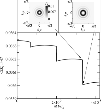
Figure 1: Total static kinetic energy of the rotating trapped Bose-Hubbard model in the rotating frame plotted versus rotation frequency for parameters ($t/U=0.03$ and $\mu/U=0.4$) giving a bulk Mott insulator surrounded by edge superfluid. The steps correspond to increasing vorticity $V=0-3$. The top panels plot the momentum distribution in the $k_{x}k_{y}$ plane for $\hbar\Omega/E_{R}=3.31\times 10^{-3}$ (left) and $3.58\times 10^{-3}$ (right).

We now examine the ground state properties of a rotating system with parameters tuned to give a Mott insulator at the trap center with a superfluid strip ($\approx 7$ sites wide) at the edge. For slow rotation (frequencies below the Mott gap) the Mott state rotates with the lattice giving zero current in the rotating frame while the superfluid has non-zero current. The main panel of Fig. (1) plots the expectation value of the static kinetic energy per particle in the rotating frame as a function of the rotation frequency. The total static lattice kinetic energy measures the net change of the ground state phase and therefore drops in steps as the superfluid increases vorticity starting from $V=0$. The circulation of the edge superfluid jumps when the number of effective flux quanta passing through the central Mott insulator increases by an integer to give critical frequencies $\Omega_{V}$ such that: $\hbar\Omega_{V}/E_{R}\approx 4V/\left(\pi^{2}|{\bm{r}}_{i^{e}}|^{2}\right).$ The steps in Fig. (1) are slightly parabolic because the hopping term in $H$ varies as $\Omega^{2}$: ${\rm Re}\left[t\exp(iA_{i,j})\right]=t(1+A_{i,j}^{2}/2+...),$ which changes the area of the Mott insulator with $\Omega$.

The change in superfluid circulation can be seen in the momentum distribution function and may therefore be observable in TOF. The momentum distribution peaks associated with the onset of superfluidity expand stepwise into rings of radius $k_{r}\approx V/(|\bm{r}_{i^{e}}|a)$. The insets of Fig. (1) show a grey scale plot of $\rho_{{\bm{k}}}$ in the $k_{x}k_{y}$ plane for two rotation frequencies. Here we see that a slight increase of frequency causes a drastic change in the shape of the momentum distribution function signaling a jump in circulation of the edge superfluid. Observation of the number of jumps (i.e. $V$), $k_{r}$, and $\Omega_{V}$ can be used to experimentally overdetermine $|{\bm{r}}_{i^{e}}|$.

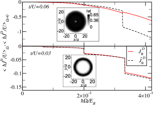
Figure 2: Main panels: The diamagnetic current, $J^{D}_{\theta}$, (solid line) and the edge approximation, $\bar{J}^{D}_{\theta}$, (dashed line) plotted in the rotating frame versus rotation frequency. Insets: The superfluid order parameter plotted in the $xy$ plane. The top panel is entirely in the superfluid phase ($t/U=0.06$ and $\mu/U=0.4$) while the bottom panel is the Mott phase with superfluid edges ($t/U=0.03$ and $\mu/U=0.4$).

We now ask if the momentum distribution can yield quantitative information related to the edge response. The superfluid rotation in the rotating frame can be thought of as a diamagnetic current. The top panel in Fig. (2) plots the excess diamagnetic current, $\langle J^{D}\rangle_{\Omega}-\langle J^{D}\rangle_{\Omega=0}$ as a function of rotational angular frequency deep in the superfluid regime of the trapped BH model with $t/U=0.06$. The inset shows a grey-scale plot of the superfluid order parameter as a function of lattice position for $\hbar\Omega/E_{R}=4.02\times 10^{-3}$. From the plot we see that there is no Mott insulator in the system but there is a vortex at the center. The solid and dashed lines indicate expectation values of $J^{D}$ and $\bar{J}^{D}$, respectively. In defining the latter we rewrite the parameter $|\bm{r}_{i^{e}}|$ in terms of an observable, $\Omega_{V}$. The step corresponds to the formation of a vortex. Here we see that the approximation made in defining $\bar{J}^{D}$ does not hold for bulk current, i.e. $\langle J_{\theta}^{\rm D}\rangle\not\approx\langle\bar{J}_{\theta}^{\rm D}\rangle.$ The superfluid order parameter varies appreciably along the direction transverse to the current and, as a result, the diamagnetic current cannot be written in the form $\mathcal{J}$. The bottom panel shows the same but for a different hopping, $t/U=0.03$, allowing for a bulk Mott insulator surrounded by edge superfluid (see inset). The dashed line reproduces the solid line indicating that $\langle J_{\theta}^{\rm D}\rangle_{e}\approx\langle\bar{J}_{\theta}^{\rm D}\rangle_{e}$ is in fact a good approximation for an edge superfluid. Here we find a small spatial variance in the superfluid order parameter along the direction transverse to the current, i.e. $\sum_{i}|\psi_{i}|^{2}(|{\bm{r}_{i}}|-|{\bm{r}_{i^{e}}}|)^{2}/\sum_{i}|\psi_{i}|^{2}\ll 1.$ We have demonstrated, by a realistic simulation, that one can generate systems obeying this small variance condition and that, as a result, the edge diamagnetic current can be written in terms of an observable, the momentum distribution. We propose that in general $\langle J_{\theta}^{\rm D}\rangle$ can be restored from observation of $\rho_{\bm{k}}$ and ${\bm{k}}$ and input parameters to yield a powerful tool for studying insulating optical lattice phases with edge states. We now discuss potential implications.

Certain insulators are characterized by a Chern number which can be related to their one dimensional edge currents Hatsugai ; Qi . As an example we assume that the Kitaev model Kitaev ; Demler_Spin ; Zoller can be realized with two component bosons in a honeycomb optical lattice. In Ref. Kitaev it was shown that the non-Abelian state can be stabilized in a uniform external magnetic field and that edge states exhibit a quantized Righi-Leduc effect. This prediction asserts that the net edge energy-current displays a thermal version of the quantum Hall effect where the transverse temperature difference, $T$, between the bulk and exterior of the sample establishes a quantized energy current along the edge: $J_{{\theta}}^{\rm E}=\nu g(\pi k_{B}T)^{2}/6h.$ Here $g=1$ for bosons and $g=1/2$ for fermions. In general we expect a clockwise and counter-clockwise energy current with an excess number of modes $\nu=\nu_{+\theta}-\nu_{-\theta}.$

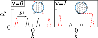
Figure 3: Schematic of the expected primary momentum distribution peaks as a function of wavevector arising from clockwise and counter-clockwise propagating edge superfluids surrounding the Kitaev optical lattice. The diamagnetic contribution to edge flow splits the peaks in an external magnetic field in the Abelian (left) and non-Abelian (right) states.

We speculate that, in principle, TOF measurements of the momentum distribution function can be used to identify chiral edge currents of constituent bosons around two dimensional insulators. Flow along the edge of the honeycomb lattice ($+\theta$ and $-\theta$) corresponds to concentric rings in TOF. If $B^{*}$ is chosen to lie at, for example, the $V=1\rightarrow 2$ crossing point the $+\theta$ and $-\theta$ modes will occupy different momentum channels resulting in two concentric rings of differing radii in the momentum distribution (Fig. (3)). This suggests that, in principle, TOF can be used to study chiral edge current and possibly identify insulators with non-zero Chern number. In practice, however, an observation of edge current in TOF pushes current experimental capabilities even for the simplest case of a BH Mott insulator.

Sufficiently accurate observations of wave vector and momentum distribution can be used as a quantitative probe but are difficult to achieve. Slow rotation induces only small $k\sim k_{r}$ modulation of the momentum distribution peaks. Small features in the momentum distribution peaks may not be resolvable experimentally because TOF measurements are ultimately limited in k-space resolution Spielman . Furthermore, $n_{s}$ can be adversely affected by interactions during TOF. Most importantly, the number of particles in edge states needs to be sufficiently large to overcome background noise in detection.

We thank C.W. Zhang for helpful discussion and ARO-DTO, ARO-LPS, and LPS-NSA for support.

References

- (1) P. Verkerk et al., Phys. Rev. Lett. 68, 3861 (1992); P. S. Jessen et al., ibid. 69, 49 (1992); A. Hemmerich et al., ibid. 70, 410 (1993).
- (2) M. Lewenstein et al., Adv. Phys. 55, 243 (2007).
- (3) W. Ketterle et al., arXiv:cond-mat/9904034.
- (4) D. Jaksch et al., Phys. Rev. Lett. 81, 3108 (1998).
- (5) M. Greiner et al., Nature (London) 415, 39 (2002).
- (6) E. Altman et al., Phys. Rev. A 70, 013603 (2004).
- (7) S. Foelling et al., Nature 434, 481 (2005).
- (8) I.B. Spielman et al., Phys. Rev. Lett. 98, 080404 (2007).
- (9) L. Pezze et al., Phys. Rev. Lett. 93, 120401 (2004).
- (10) C. D. Fertig et al., Phys. Rev. Lett. 94, 120403 (2005).
- (11) S. Tung et al., Phys. Rev. Lett. 97, 240402 (2006).
- (12) R. Dum et al., Phys. Rev. Lett. 76, 1788 (1996); S. K. Dutta et al., ibid. 83, 1934 (1999); D. Jaksch et al., New J. Phys. 5, Art. 56 (2003); K. Osterloh et al., Phys. Rev. Lett. 95, 010403 (2005); G. Juzeliunas et al., Phys. Rev. A 73, 025602 (2006).
- (13) A. S. Sorensen et al., Phys. Rev. Lett. 94, 086803 (2005).
- (14) K. Goral et al., Phys. Rev. Lett. 88, 170406 (2002).
- (15) V.W. Scarola et al., Phys. Rev. Lett. 95, 033003 (2005).
- (16) A. Isacsson et al., Phys. Rev. A. 72, 053604 (2005).
- (17) A. Kitaev, Ann. Phys. 321, 2 (2006).
- (18) L.-M. Duan et al., Phys. Rev. Lett. 91, 090402 (2003).
- (19) A. Micheli et al., Nature Physics, 2, 341 (2006).
- (20) C. Wu et al., Phys. Rev. A 69, 043609 (2004).
- (21) R. Bhat et al., Phys. Rev. Lett. 96, 060405 (2006); Phys. Rev. A 74, 063606 (2006).
- (22) Y. Hatsugai et al., Phys. Rev. Lett. 71, 3697 (1993).
- (23) Xiao-Liang Qi et al., Phys. Rev. B 74, 045125 (2006).
- (24) R. Peierls, Quantum Theory of Solids (Oxford University Press, New York, 1955).
- (25) D. J. Scalapino et al., Phys. Rev. Lett. 68, 2830 (1992).
- (26) J. Grondalski et al., Opt. Express 5, 249 (1999).
- (27) V. A. Kashurnikov et al., Phys. Rev. A 66, 031601(R) (2002).
- (28) D.S. Rokhsar et al., Phys. Rev. B 44, 10328 (1991).
- (29) J. Zakrzewski, Phys. Rev. A 71, 043601 (2005).