Josephson vortex motion as a source for dissipation of superflow of e-h pairs in bilayers

Abstract

It is shown that in a bilayer excitonic superconductor dissipative losses emerge under transmission of the current from the source to the load. These losses are proportional to the square of the interlayer tunneling amplitude and independent on the value of the input current. The case of quantum Hall bilayer is considered. The bilayer may work as a transmission line if the input current exceeds certain critical value. The input current higher than critical one induces Josephson vortices in the bilayer. The difference of electrochemical potentials is required to feed the load and it forces Josephson vortices to move. The state becomes non-stationary that leads to dissipation.

,

1 Introduction

Among the phenomena that demonstrate bilayer electron systems in semiconductor heterostructures considerable attention is given to superfluidity of electrons-hole (e-h) pairs with components belonging to different layers (see, for instance, [1]). A flow of electron-hole pairs in the bilayer is equivalent to two oppositely directed electrical currents in the layers. Therefore, the superflow of such pairs is a kind of superconductivity. For the first time the effect was considered in Refs. [2, 3] for bilayers where one layer is of the electron-type conductivity and the other layer - of the hole-type one (electron-hole bilayers). The next important step was the prediction of the e-h superfluidity for the systems where the conductivity of both layers is of the same type [4, 5]. In that case the bilayer should be subjected by a strong perpendicular to the layers magnetic field. If the total filling factor of the Landau levels is $\nu=1$ the number of electrons in one layer coincides with the number of holes in the other layer (the empty states in the lowest Landau level play the role of holes) and the Coulomb attraction between electrons and holes results in a formation of bound pairs. Note that the description of electron-hole pairing in electron-electron bilayers in a quantized magnetic field is close to one developed earlier for the quantum Hall electron-hole bilayers [6, 7, 8]

The prediction [4, 5] has inspired considerable increase of interest to the study of this phenomenon, both theoretically [9, 10, 11, 12, 13, 14, 15, 16, 17] and experimentally[18, 19, 20, 21, 22, 23, 24, 25, 26]. The results of recent experimental investigations of quantum Hall bilayers support the idea on superfluidity of e-h pairs in these systems. In particular, in the counterflow experiments a huge increase of a longitudinal conductivity was observed[18, 19, 20]. Other important observations are a large low bias tunnel conductivity [21], that also takes place in bilayers with large imbalance of filling factors [26], the Goldstone collective mode [22], the quantized Hall drag between the layers [23], the interlayer drag [24] and the interlayer critical supercurrent [25] in the Corbino disk geometry. The low temperature properties of optically generated indirect excitons in bilayers in zero magnetic field were also studied experimentally [27, 28], and specific features in the photoluminescence spectra accounted for the Bose-Einstein condensation of electron-hole pairs have been observed. Recent important contribution into this topic is connected with the idea of using two graphene layers separated by a dielectric layer [29, 30, 31, 32] instead of GaAs heterostructures. It is expected [29] that in graphene systems in zero magnetic field superconductivity of e-h pairs may take place at rather high temperatures.

A superfluid state of electron-hole pairs in quantum Hall bilayers can be considered as a state with spontaneous interlayer phase coherence between the electrons. The coherent phase $\varphi$ is the phase of the order parameter for the electron-hole pairing, and gradient of the phase $\varphi$ determines the value of the supercurrent in the layer (planar supercurrent).

The bilayer system in the counterflow setup[18, 19, 20] can be used as a double-wire circuit that transmits the current from the source to the load. If the transmission is provided by superfluid e-h pairs one can expect that such a line will work as a usual superconducting transmission line. Nevertheless, genuine superconductivity was not achieved in the counterflow experiments. A finite resistance can be accounted for a disorder that results in a finite concentration of planar vortices in the bilayer [33, 34]. But there is another principal circumstance that may forbid genuine superconductivity in such a transmission line. To support nonzero current in the load circuit the difference of electrochemical potentials between the layers is required. This difference results in a temporal dependence of the phase $\varphi$. The state with the spontaneous interlayer phase coherence emerges if the layers are situated rather close to each other (at the distance less or of other of the magnetic length). Therefore, nonzero interlayer tunneling is always present in real physical systems. At nonzero interlayer tunneling amplitude the difference of electrochemical potentials results in appearance of an a.c. Josephson current and the state becomes non-stationary one. As was shown in [35] dissipative losses emerge in the non-stationary state. The situation is different for the loop and for the load geometry [36]. The steady state is not possible in the loop geometry Fig. 1b (that corresponds to the transmission line [18, 19, 20]) but it can be realized in the load geometry shown in Fig. 1a under condition that the difference of the electrochemical potential of the layers is tuned to zero.

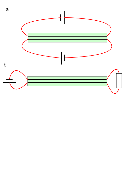
Figure 1: The load (a) and the loop (b) setups.

The load geometry [36] is an appropriate setup for the observation of the superfluidity of e-h pairs but it cannot be used for the transmission of the current from the source to the load. In more complicated circuits, e.g. made of a stack of bilayers, non-dissipative transmission of the energy is not possible, as well. Indeed, a bilayer with zero difference of electrochemical potentials can be shunted at both ends without any impact on electrical currents and voltages in external circuits. It means that the removal of such a bilayer from the circuit cannot change its working parameters, including the power of losses. An example of such shunting is shown in Fig. 2. The only setup where superfluid properties of e-h pairs may lead to lowering of dissipation is the system with nonzero difference of electrochemical potentials between the layers. While non-stationary states are not free from dissipation, the losses can be exponentially small and one can say about almost superconducting state.

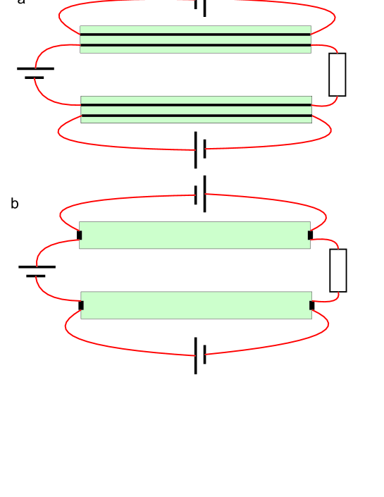
Figure 2: A circuit with a stack of bilayers (a) and an equivalent circuit with shunted bilayers (b)

In this paper we consider dissipative processes in the bilayer in the loop geometry and find the conditions at which the losses are small. The state with a.c. Josephson and planar supercurrents that emerges in the bilayer can be described as a moving chain of Josephson vortices. Under such a motion two mechanisms of dissipation come into play. They are the second viscosity that results in dissipation in the non-stationary regime and Joule losses caused by a.c. electrical fields that emerge due to spatial and temporal variation of the interlayer voltage.

In Sec. 2 starting from the microscopic Hamiltonian and using the BCS-like many-particle wave function we derive the stationary continuity equation. In Sec. 3 stationary vortex states are considered and the problem of the lower critical current is addressed. In Sec. 4 the state with moving vortices is investigated and the power of losses caused by such a motion is computed. We find the power of losses is proportional to the square of the tunneling amplitude and depends nonlinearly on the resistance of the load.

2 The model

Let us consider a bilayer electron system subjected by a strong perpendicular to the layers magnetic field $B$. The filling factors of the layers satisfy the condition $\nu_{1}+\nu_{2}=1$, where $\nu_{i}=2\pi\ell^{2}n_{i}$, $n_{i}$, are the electron densities in the layers, and $\ell=\sqrt{\hbar c/eB}$ is the magnetic length. Implying the energy gap between the Landau levels $\hbar\omega_{c}$ ($\omega_{c}$ is the cyclotron frequency) be larger than the Coulomb energy $e^{2}/\varepsilon\ell$ ($\varepsilon$ is the dielectric constant) we use the lowest Landau level approximation. In this approximation the Hamiltonian of the system has the form

$$H=-t\sum_{X}\left(a^{+}_{1X}a_{2X}+{\textrm{H}.c.}\right)+\frac{1}{2S}\sum_{n,n^{\prime}=1,2}\sum_{\bf q}V_{n,n^{\prime}}({\bf q})[\rho_{n}({\bf q})\rho_{n^{\prime}}(-{\bf q})-\delta_{nn^{\prime}}\rme^{-\frac{q^{2}\ell^{2}}{2}}\rho_{n}(0)].$$ (1)

Here $a^{+}_{nX}$, $a_{nX}$ are the creation and annihilation operators for the electrons in the $n$-th layer, $X$ is the guiding center of the orbit, $S$ is the area of the layer, $t$ is the interlayer tunneling amplitude, $\rho_{n}({\bf q})=\sum_{X}a^{+}_{n,X+q_{y}\ell^{2}/2}a_{n,X-q_{y}\ell^{2}/2}\rme^{\rmi q_{x}X-q^{2}\ell^{2}/4}$ is the operator for the Fourier component of the electron density, and $V_{n,n^{\prime}}({\bf q})=({2\pi e^{2}}/{\varepsilon q})\exp(-qd|n-n^{\prime}|)$ is the Fourier component of the Coulomb potential ($d$ is the distance between the layers). In what follows we consider the bilayer of a rectangle shape ($S=L_{x}\times L_{y}$) with the planar currents directed parallel to the $x$ axis.

The state with the interlayer phase coherence is described by the wave function

$$|\Psi\rangle=\prod_{X}\left(ua_{1X}^{+}+va_{2X}^{+}\right)|0\rangle,$$ (2)

where the coefficients $u$ and $v$ satisfy the condition $|u|^{2}+|v|^{2}=1$. The physical meaning of this function and its applicability for a description of the superfluid state of $e-h$ pairs in quantum Hall bilayers was discussed in [9, 10, 11] and in a number of further papers. Here we just remind the main points. The function (2) can be presented in another equivalent form

$$|\Psi\rangle=\prod_{X}\left(u+va_{2X}^{+}h^{+}_{1X}\right)|vac\rangle,$$ (3)

where $h^{+}_{n}=a_{n}$ is the creation operator for the hole, and the vacuum state $|vac\rangle$ is the state in which layer 1 is fully occupied and the layer 2 is empty ($\nu_{1}=1$ and $\nu_{2}=0$). It was shown [8] that the function (2), (3) corresponds to the ground state of the Hamiltonian (1) in the limit $d/\ell\to 0$. One can see that the function (3) is the standard BCS form for the exciton condensate. The exciton is thought of as an electron in the layer 2 bound to a hole in the layer 1. One can show (see, for instance, [37]) that in the first quantizied language the function (2),(3) is reduced to the (111) Halperin wave function. At finite $d/\ell$ the state (2), (3) is not the exact ground state. Nevertheless, numerical studies show (see e.g. Ref. [38]) that at $d/l<0.5$ the overlap with the exact ground state is close to hundred percents. For the system with given filling factors of the layers the $u-v$ coefficients in (2), (3) read as $u=\sqrt{\nu_{1}}$ and $v=e^{i\varphi}\sqrt{\nu_{2}}$. In the absence of the interlayer tunneling the energy of the state (2), (3) does not depend on the phase $\varphi$. In case of spatially dependent phase $\varphi=\varphi(X)$ the function (2), (3) describes the state with nonzero counterflow electrical currents in the layers (see [9]).

The order parameter for the exciton condensate at $T=0$ is

$$\Delta(X)=\langle\Psi|a_{2X}h_{1X}|\Psi\rangle=u^{*}_{X}v_{X}=\Delta_{0}e^{i\varphi(X)},$$ (4)

where $\Delta_{0}=\sqrt{\nu_{1}(1-\nu_{1})}$. Due to the absence of the kinetic energy of carriers in the Landau level the self-consistence equation for the order parameter at $T=0$ is reduced to an algebraic equation. At nonzero temperature the equation for the order parameter takes a self-consistent form ([6, 39]) from which the temperature dependence of the order parameter and the mean-field critical temperature can be obtained. But due to the two-dimensional nature of the bilayer excitons the temperature of transition into the superfluid state is not the mean-field critical temperature, but the Berezinskii-Kosterlitz-Thouless transition temperature $T_{\rm BKT}\approx\pi\rho_{s}/2$, see [9] (the definition of the superfluid stiffness $\rho_{s}$ is given below).

If the gradient of the phase is small in comparison with the inverse magnetic length, the energy of the system $E=\langle\Psi|H|\Psi\rangle$ can be written in the continuous approximation

$$E=E_{0}+\int\rmd^{2}r\left[\frac{1}{2}\rho_{\rm s}\left(\frac{\rmd\varphi}{\rmd x}\right)^{2}-\frac{\tilde{t}}{2\pi\ell^{2}}(\cos\varphi-1)\right],$$ (5)

where $E_{0}$ is the energy of the ground state, $\tilde{t}=2t\Delta_{0}$ is the tunneling energy and

$$\rho_{\rm s}=\Delta_{0}^{2}\frac{e^{2}}{4\pi\varepsilon\ell}\left[\sqrt{\frac{\pi}{2}}\exp\left(\frac{d^{2}}{2\ell^{2}}\right){\rm erfc}\left(\frac{d}{\ell\sqrt{2}}\right)\left(1+\frac{d^{2}}{\ell^{2}}\right)-\frac{d}{\ell}\right]$$ (6)

is the energy parameter called the superfluid stiffness. The superfluid stiffness can also be presented in a more familiar form $\rho_{\rm s}=\hbar^{2}n_{\rm s}/m_{B}$, where $n_{\rm s}$ is the superfluid density of the pairs, and $m_{B}$ is the magnetic mass of the pair (see, for instance, [14]). One can see from (5) that at nonzero tunneling amplitude the ground state corresponds to the phase $\varphi=0$. But it does not mean the fixation of the phase and the absence of electrical currents. It means that the planar current should be accompanied with the interlayer current.

Varying the energy (5) with respect to the phase and equating the result to zero we obtain the equation

$$-\frac{e\rho_{\rm s}}{\hbar}\frac{\rmd^{2}\varphi}{\rmd x^{2}}+\frac{e}{\hbar}\frac{\tilde{t}}{2\pi\ell^{2}}\sin\varphi=0.$$ (7)

The first term in Eq. (7) is the 2D divergence of the density of the planar supercurrent

$$j_{1}=-j_{2}=-\frac{e\rho_{\rm s}}{\hbar}\frac{\rmd\varphi}{\rmd x}.$$ (8)

The expression for the planar current can be obtained from the gauge invariance arguments (see [15, 40]).

One can see the Eq. (7) is the stationary continuity equation

$$\frac{\rm dj_{1}}{\rm dx}+I_{1\to 2}=0,$$ (9)

where

$$I_{1\to 2}=\frac{e}{\hbar}\frac{\tilde{t}}{2\pi\ell^{2}}\sin\varphi$$ (10)

is the density of the interlayer supercurrent flowing from the layer 1 to the layer 2.

The coherent electrical current between the layers corresponds to nonzero $\varphi$, in a close analogy with the Josephson effect between two bulk superconductors. The difference is that $\varphi$ is the phase of a given condensate, but not the phase difference for two condensates.

Eq. (7) can be presented in the form

$$\frac{\rmd^{2}\varphi}{\rmd x^{2}}=\frac{1}{\lambda^{2}}\sin\varphi,$$ (11)

where $\lambda=\ell\sqrt{2\pi\rho_{\rm s}/\tilde{t}}$ is the Josephson length. As follows from Eq. (11), the gradient of the phase is of order of $\lambda^{-1}$. Therefore, the continuity approximation (5) requires $\lambda\gg\ell$. This inequality is fulfilled if the tunneling amplitude $t$ is much smaller than the Coulomb energy $e^{2}/\varepsilon\ell$ and the filling factor $\nu$ is not very close to zero.

3 Stationary vortex state and lower input critical current

The problem of the lower critical current was already discussed in a number of papers [12, 15, 41]. Here we revisit this question again with the aim to give a more accurate definition of the lower critical current and to clarify some discrepancies in [12, 15, 41].

Let us consider the following situation. A fixed input current from a source is entered into one layer in a given (source) end of the system. There is no difference between the electrochemical potentials of the layers and the stationary state is realized. The current withdrawn from the adjacent layer at the same end is equal to the input current. The values of the output and input currents at the opposite (load) end are also equal to each other, but, in general, they may differ from currents at the source end. For instance, such a situation corresponds to the load geometry [36] (then all input and output currents are equal to one another). In the loop geometry the stationary state can be realized if the load has zero resistance (superconducting load), or if an additional source in the load circuit provides zero difference of electrochemical potentials between the layers.

Depending on the values of the input currents two qualitative different stationary current patterns can emerge: either the planar and interlayer currents are nonzero in the whole bilayer, or the currents decrease exponentially with the distance from the ends and there is no currents in the internal part of the bilayer. We define the lower critical input current as the current at which the switching between these two regimes occurs. If the input currents at both ends are lower than the critical one the second pattern is realized and the interior part of the bilayer is not involved into the transmission of the current (the cutting of the bilayer does not change currents in outer circuits). If one or both input currents exceed $j_{c}$ the first pattern emerges.

Let us switch to the quantitative analysis. Eq. (11) coincides in form with the equation of motion for a nonlinear pendulum

$$\frac{\rmd^{2}\varphi}{\rmd t^{2}}=\omega_{0}^{2}\sin\varphi,$$ (12)

where $\omega_{0}$ is the resonant frequency of the pendulum, and $\varphi$ is the angle coordinate counted from the unstable equilibrium point. The formal coincidence of Eq. (11) and Eq. (12) allows us to describe the stationary states in the bilayer basing on known behavior of a nonlinear pendulum.

Depending on the energy, the pendulum oscillates, completes a full revolution in infinite time, or rotates. The maximum angular velocity $\omega_{\rm m}$ of the pendulum (velocity at $\varphi=\pi$) is proportional to the square root of the energy and it increases if one switches from the oscillating to the rotating regime. For the full revolution in infinite time the maximum angular velocity $\omega_{\rm m}=2\omega_{0}$.

The time dependent angular velocity in the pendulum problem corresponds to the space dependent planar supercurrent in the bilayer problem. The counterpart of the full revolution regime is a state with one Josephson vortex. In this state the planar and the interlayer supercurrents are given by the expressions

$$j_{1}=-j_{2}=j_{\rm c}{\rm sech}\left(\frac{x-x_{0}}{\lambda}\right),$$ (13)

$$I_{1\to 2}=\frac{j_{\rm c}}{\lambda}\,{\rm sech}\left(\frac{x-x_{0}}{\lambda}\right)\tanh\left(\frac{x-x_{0}}{\lambda}\right),$$ (14)

where $x_{0}$ is the vortex center, and

$$j_{\rm c}=\frac{e\rho_{\rm s}}{\hbar}\frac{2}{\lambda}$$ (15)

is the maximum value of planar supercurrent in the single vortex state (it is reached at the center of the vortex). Note that Eq. (15) can be obtained directly from Eq. (8) under accounting the correspondences $(\rmd\varphi/\rmd x)_{\rm max}\Leftrightarrow\omega_{\rm m}=2\omega_{0}$ and $\omega_{0}\Leftrightarrow 1/\lambda$.

The counterpart of the rotation regime is the state with many equally distanced Josephson vortices with the same sign of vorticity. The supercurrents in this state read as

$$j_{1}=-j_{2}=\frac{j_{\rm c}}{\sqrt{\eta}}{\rm dn}\left(\frac{x}{\lambda\sqrt{\eta}},\eta\right),$$ (16)

$$I_{1\to 2}=\frac{j_{\rm c}}{\lambda}\,{\rm sn}\left(\frac{x}{\lambda\sqrt{\eta}},\eta\right){\rm cn}\left(\frac{x}{\lambda\sqrt{\eta}},\eta\right).$$ (17)

The analog of the oscillating motion of the pendulum is the multivortex state with vortices of alternating vorticity:

$$j_{1}=-j_{2}={j_{\rm c}}{\sqrt{\eta}}{\rm cn}\left(\frac{x}{\lambda},\eta\right),$$ (18)

$$I_{1\to 2}=\frac{j_{\rm c}\sqrt{\eta}}{\lambda}{\rm dn}\left(\frac{x}{\lambda},\eta\right){\rm sn}\left(\frac{x}{\lambda},\eta\right).$$ (19)

In Eqs. (16), (18) ${\rm dn}(u,\eta)$, ${\rm cn}(u,\eta)$ and ${\rm sn}(u,\eta)$ are the Jacobi elliptic functions and the parameter $\eta$ belongs to the interval $(0,1)$.

The boundary condition for the bilayer problem is the condition on the gradients of the phase. This condition alone does not determine an unique current state. The system chooses the state that at given input currents has the lowest energy. Direct calculation shows that the energies of the multivortex state (16) and (18) are both higher than the energy of the single vortex state (13). It is obvious result since the energy of any multivortex state is proportional to the number of vortices.

Here we should emphasize the difference between the pendulum problem and the bilayer problem. The energy of the pendulum is the integral of motion of Eq. (12), while the bilayer energy (5) is not the first integral of Eq. (11). Therefore, the analogy between these two problems fails if one analyzes the energies of different states.

One can see that the planar supercurrent may exceed $j_{\rm c}$ only in the state (16). Therefore, if the input current $j_{\rm in}$ is higher than $j_{\rm c}$ the multivortex state (16) is realized. The parameter $\eta$ is determined by the conditional minimum of energy and it is equal to $\eta=(j_{\rm c}/j_{\rm in})^{2}$. The density of the Josephson vortices increases under increase of the input current.

If the input current is smaller than $j_{\rm c}$ the state with one incomplete vortex centered outside the bilayer satisfies the boundary condition and corresponds to the minimum of energy. Thus, the state realized at $j_{\rm in}\leq j_{\rm c}$ is the state with zero supercurrents inside the bilayer.

The vortex state with alternating vorticities (18) is not realized in the bilayers. It may satisfy the boundary conditions only at $j_{\rm in}<j_{\rm c}$, but its energy is larger than the energy of the state with one vortex. It contradicts the conclusion of Ref. [41], but in Ref. [41] the first integral of Eq. (11) was incorrectly identified with the energy.

Thus, the quantity (15) is just the lower input critical current defined above.

At $j_{\rm in}\gg j_{\rm c}$ the overlapping between the vortices is large and the current pattern is approximated by a sum of large d.c part and small harmonic a.c. part:

$$\varphi\approx\pi-kx-A_{\varphi}\sin kx,$$ (20)

$$j_{1}=-j_{2}\approx\frac{j_{\rm in}}{1+A_{\varphi}}\left(1+A_{\varphi}\cos kx\right),$$ (21)

$$I_{1\to 2}\approx\frac{e}{\hbar}\frac{\tilde{t}}{2\pi\ell^{2}}\sin kx,$$ (22)

where

$$k=\frac{\pi j_{\rm in}}{j_{\rm c}\lambda K\left(\frac{j_{c}^{2}}{j_{\rm in}^{2}}\right)}\approx\frac{2j_{\rm in}}{j_{\rm c}\lambda},\quad A_{\varphi}=\frac{j_{\rm c}^{2}}{4j_{\rm in}^{2}}.$$

Here $K(\eta)$ is the complete elliptic integral of the first kind.

To conclude this section we note that at small input current (lower than $j_{\rm c}$) the tunneling provides shunting of the bilayer at both ends. It means that the load geometry experiments proposed in [36] for the observation of e-h superfluidity should be done at large currents.

4 Vortex motion and dissipation

As was already discussed in the introduction, the stationary state cannot be realized in the bilayer transmission line with nonzero load resistance. But even in case of non-stationary currents inside a bilayer the currents in external circuits may remain stationary one. The latter occurs if the contacts between the layers and the external wires average the input and output currents.

In such a situation the term ”lower critical current” slightly changes its meaning. The average current depends on the density of vortices and can be smaller than $j_{\rm c}$. But the input current higher than critical one is required at the beginning of the process to induce a chain of moving vortices.

To study the non-stationary vortex state we will use the set of equations for the phase of the order parameter $\varphi$ and for the local difference of the electrochemical potentials between the layers $eV$, where $V$ is the local interlayer voltage. The first equation comes from the non-stationary continuity equation

$$e\frac{\partial\tilde{n}}{\partial t}+\frac{\partial j_{1}^{\rm s}}{\partial x}+I_{1\to 2}+\frac{\partial j_{1}^{\rm n}}{\partial x}=0.$$ (23)

Here $\tilde{n}$ is the excess local density of electron-hole pairs. It is connected with the local voltage by the capacitor equation

$$\frac{e\tilde{n}}{V}=C,$$ (24)

where

$$C=\frac{\varepsilon}{4\pi d}\frac{1}{1-\frac{\ell}{d}\sqrt{\frac{\pi}{2}}\left[1-\exp\left(\frac{d^{2}}{2\ell^{2}}\right){\rm erfc}\left(\frac{d}{\ell\sqrt{2}}\right)\right]}$$ (25)

is the effective capacity of the bilayer system per unit area. The effective capacity takes into account the exchange interaction between the layers and differs from the classical capacity by the additional factor (the second factor in Eq. (25)). It can be obtained from the dependence of the energy on the filling factor imbalance (see, e.g. [39]). The superscripts ”s” and ”n” in Eq. (23) stand for the planar supercurrent and for the planar current of quasiparticles. The current of qusiparticles is taken into account in Eq. (23) because it is induced by a.c. planar electrical fields that emerge in the non-stationary state. These fields equal to $E_{1}=-E_{2}=-(1/2)\partial V/\partial x$ and the quasiparticle current can be presented in the form $j_{1}^{(n)}=-(\sigma_{n}/2)\partial V/\partial x$, where $\sigma_{n}$ is the quasiparticle conductivity. We do not take into account the normal component of the interlayer current because the normal tunneling is suppressed due to discreteness of the Landau levels.

The second equation on $\varphi$ and $V$ can be derived from the equations of superfluid hydrodynamics [42], namely, from the equation for the superfluid velocity with dissipative terms. The linearized version of this equation reads as

$$\frac{\partial{\bf v}_{\rm s}}{\partial t}=-\nabla\mu_{m}+\nabla\left[\zeta_{3}\nabla\cdot n_{\rm s}({\bf v}_{\rm s}-{\bf v}_{\rm n})+\zeta_{4}\nabla\cdot{\bf v}_{\rm n}\right],$$ (26)

where $\mu_{m}$ is the chemical potential per unit mass $\mu_{m}=\mu/m$ ($m$ is the mass of the Bose particle), $n_{\rm s}$ is the superfluid density, ${\bf v}_{\rm n}$ is the velocity of the normal component, $\zeta_{3}$, $\zeta_{4}$ are the second viscosity parameters. To apply Eq. (26) for the description of the bilayer electron-hole superfluidity one should replace the divergence of the superfluid flow in (26) with the divergence of the planar supercurrent plus the tunnel supercurrent: $\nabla(n_{\rm s}{\bf v}_{\rm s})\Rightarrow(1/e)(\partial j_{1}^{\rm s}/\partial x+I_{1\to 2})$, and substitute the difference of the electrochemical potentials instead of the chemical potential $\mu\Rightarrow eV$. Using Eqs. (10), (8), and the expression for the superfluid velocity ${\bf v}_{\rm s}=-\hbar\nabla\varphi/m$ (the negative sign is because the phase $\varphi$ describes the coherence between the electrons), we obtain

$$\nabla\left(\hbar\frac{\partial{\varphi}}{\partial t}\right)=\nabla\left[eV+\zeta_{3}\frac{m}{2\pi\ell^{2}\hbar}\left(2\pi\ell^{2}\rho_{\rm s}\frac{\partial^{2}\varphi}{\partial x^{2}}-\tilde{t}\sin\varphi\right)+\Or(v_{\rm n})\right].$$ (27)

The quantity $\Or(v_{\rm n})$ in Eq. (27) stands for the term caused by the motion of the normal component. Below we will neglect the $\Or(v_{\rm n})$ term. One can show that this term yields the correction to the power of losses quadratic in the dissipative coefficients, while the leading term is linear in these coefficients. Since we are interested in the vortex solution, the gradients in (27) can be omitted.

Thus, we obtain the following set of equations for $\varphi$ and $V$

$$C\frac{\partial V}{\partial t}=\frac{e}{\hbar}\rho_{\rm s}\frac{\partial^{2}\varphi}{\partial x^{2}}-\frac{e}{\hbar}\frac{\tilde{t}}{2\pi\ell^{2}}\sin\varphi+\frac{\sigma_{\rm n}}{2}\frac{\partial^{2}V}{\partial x^{2}},$$ (28)

$$\hbar\frac{\partial\varphi}{\partial t}=eV+\alpha_{\varphi}\left(2\pi\ell^{2}\rho_{\rm s}\frac{\partial^{2}\varphi}{\partial x^{2}}-\tilde{t}\sin\varphi\right).$$ (29)

The coefficient $\alpha_{\varphi}=\zeta_{3}m/2\pi\ell^{2}\hbar$ in Eq. (29) is the second superfluid viscosity expressed in dimensionless units (with $m=m_{B}$, the magnetic mass of the e-h pair). Eqs. (28), (29) contain two terms responsible for the dissipation. The term proportional to $\sigma_{\rm n}$ describes the Joule losses caused by a.c. quasiparticle currents, and the term proportional $\alpha_{\varphi}$ - the losses caused by the second viscosity. The equations with the same form of dissipative terms were used in [43]. Eq. (29) was also obtained in Ref. [44] for the electron-hole bilayers in zero magnetic field in the ”dirty” limit.

The channels of dissipation caused by the second viscosity and quasiparticle currents are present in any superfluid system, but they do not result automatically in dissipative losses. One can see that in the stationary regime the dissipative terms in Eqs. (28), (29) equal to zero. The losses appear under presence of additional factors. For the bilayer transmission line the main factor is non-stationarity of the interlayer and the planar supercurrents.

As was shown in the previous section, the input current may induce Josephson vortices in the bilayer system. At nonzero difference of the electrochemical potentials the vortices begin to move from the source to the load. Neglecting for a moment the dissipative terms we obtain from Eqs. (28), (29) the following equation for the phase

$$\frac{\partial^{2}\varphi}{\partial\xi^{2}}-\frac{\partial^{2}\varphi}{\partial\tau^{2}}=\sin\varphi,$$ (30)

where the dimensionless variables $\xi=x/\lambda$ and $\tau=t/\tau_{0}$ ($\tau_{0}=(\hbar\ell/e)\sqrt{2\pi C/\tilde{t}}$) are used. Eq. (30) has the solution $\varphi(\xi,\tau)=\phi(\xi-\beta\tau)$, where $\beta\neq 1$ and $\phi(u)$ satisfies the equation

$$\frac{\partial^{2}\phi}{\partial u^{2}}=\frac{1}{1-\beta^{2}}\sin\phi$$ (31)

that up to the notations coincides with Eq. (11). Using the results of Sec. 3 we obtain the following expression for the planar current and for the interlayer voltage

$$j_{1}^{\rm s}(x,t)=\frac{2e}{\hbar}\rho_{\rm s}k\ {\rm dn}\left(kx-\omega t,\eta\right),$$ (32)

$$V(x,t)=\frac{2\hbar\omega}{e}{\rm dn}\left(kx-\omega t,\eta\right),$$ (33)

where

$$k=\frac{1}{\lambda\sqrt{\eta|1-\beta^{2}|}},\quad\omega=\frac{\beta}{\tau_{0}\sqrt{\eta|1-\beta^{2}|}}.$$ (34)

Eq. (32) describes the moving vortex lattice. The velocity of motion is

$$u_{\rm v}=\frac{\omega}{k}=\frac{e^{2}}{\hbar^{2}}\rho_{\rm s}\frac{\langle V\rangle}{\langle j_{1}^{\rm s}\rangle}=\frac{e^{2}\rho_{\rm s}RL_{y}}{\hbar^{2}}.$$ (35)

Here and below $\langle\ldots\rangle$ means the time average. In Eq. (35) $R$ is the resistance of the load (we imply the Ohm law $\langle V\rangle=RL_{y}\langle j_{1}^{\rm s}\rangle$ for the load circuit). One can see that the vortex velocity is proportional to the load resistance and does not depend on the input current. The parameter $\beta=u_{v}\tau_{0}/\lambda$ is also proportional to the load resistance.

Let us switch to the case of small but nonzero dissipation. The power of losses can be obtained from the common expression for the Joule losses

$$\Delta P=L_{y}\left\langle\int_{0}^{L_{x}}dx\left[I_{1\to 2}V+(j_{1}^{\rm s}+j_{1}^{\rm n})\left(-\frac{\partial V}{\partial x}\right)\right]\right\rangle.$$ (36)

Integrating (36) by parts and taking into account the continuity equation (23) we obtain the obvious result that the power of losses is the input power minus the output power:

$$\Delta P=(j_{\rm in}-j_{\rm out})V_{0}L_{y}.$$ (37)

Here $j_{out}$ is the output planar current, and $V_{0}$ is the voltage in the output circuit (that coincides with the voltage applied to the bilayer system at the input end). In deriving (37) we take into account that $\langle V(\partial V/\partial t)\rangle=0$ for any function $V(x,t)$ periodic in $t$.

The difference between the input and the output average currents emerges if the average value of the interlayer current $\bar{I}=\langle I_{1\to 2}\rangle$ differs from zero. In what follows we consider the case where the power of losses is much smaller than the input power. In this case one can neglect the dependence of $\bar{I}$ on $x$ and approximate the difference $j_{\rm in}-j_{\rm out}$ as $j_{\rm in}-j_{\rm out}=L_{x}\bar{I}$. Then the power of losses reads as

$$\Delta P=\bar{I}V_{0}S.$$ (38)

The quantity $\bar{I}$ can be found from the solutions of Eqs. (28), (29). Here we consider the case of large input current $j_{\rm in}\gg j_{\rm c}$. In this case one can seek for a solution of Eqs. (28), (29) in the following form

$$\varphi(x,t)=\omega t-kx+A_{\varphi}\sin(\omega t-kx)+B_{\varphi}\cos(\omega t-kx),$$ (39)

$$V(x,t)=V_{0}\left(1+A_{V}\sin(\omega t-kx)+B_{V}\cos(\omega t-kx)\right),$$ (40)

where $\omega=eV_{0}/\hbar$, and the quantity $k$ is connected with the planar supercurrent by the relation $\langle j_{1}^{\rm s}\rangle=e\rho_{\rm s}k/\hbar$. Substituting Eqs. (39), (40) into Eqs. (28) (29) and neglecting the terms quadratic in $\tilde{t}$ we obtain the coefficients $A_{\varphi}$, $B_{\varphi}$, $A_{V}$, $B_{V}$ in the leading order in $\tilde{t}$:

$$A_{\varphi}=-\frac{\tilde{t}}{2\pi\ell^{2}k^{2}\rho_{\rm s}}\frac{(1-\beta^{2}+2\pi\ell^{2}k^{2}\alpha_{\varphi}\tilde{\sigma})(1+2\pi\ell^{2}k^{2}\alpha_{\varphi}\tilde{\sigma})+\alpha_{\varphi}\frac{V_{0}}{V_{C}}\left(\alpha_{\varphi}\frac{V_{0}}{V_{C}}+\tilde{\sigma}\frac{V_{0}}{V_{\rho}}\right)}{D},$$ (41)

$$B_{\varphi}=\frac{\tilde{t}}{2\pi\ell^{2}k^{2}\rho_{\rm s}}\frac{\tilde{\sigma}\frac{V_{0}}{V_{\rho}}\left(1+2\pi\ell^{2}k^{2}\alpha_{\varphi}\tilde{\sigma}\right)+\alpha_{\varphi}\frac{V_{0}}{V_{C}}\beta^{2}}{D},$$ (42)

$$A_{V}=-\frac{\tilde{t}}{2\pi\ell^{2}k^{2}\rho_{\rm s}}\frac{\alpha_{\varphi}\frac{V_{0}}{V_{C}}+\tilde{\sigma}\frac{V_{0}}{V_{\rho}}}{D},$$ (43)

$$B_{V}=-\frac{\tilde{t}}{2\pi\ell^{2}k^{2}\rho_{\rm s}}\frac{1+2\pi\ell^{2}k^{2}\alpha_{\varphi}\tilde{\sigma}-\beta^{2}}{D},$$ (44)

where

$$D=\left(1-\beta^{2}+2\pi\ell^{2}k^{2}\alpha_{\varphi}\tilde{\sigma}\right)^{2}+\left(\alpha_{\varphi}\frac{V_{0}}{V_{C}}+\tilde{\sigma}\frac{V_{0}}{V_{\rho}}\right)^{2},$$ (45)

and the following notations are used

$$\beta^{2}=\frac{CV_{0}^{2}}{\rho_{\rm s}k^{2}},\quad V_{C}=\frac{e}{2\pi\ell^{2}C},\quad V_{\rho}=\frac{\rho_{\rm s}}{e},\quad\tilde{\sigma}=\frac{\sigma_{\rm n}\hbar}{2e^{2}}.$$ (46)

Note the equivalence of $\beta$ in (46) and the definition of $\beta$ given above.

One can see that at $\tilde{t}=0$ all the coefficients $A_{\varphi}$, $B_{\varphi}$, $A_{V}$, $B_{V}$ are equal to zero that reflects the absence of vortices in the bilayers with zero interlayer tunneling.

Using Eqs. (10) and (39) one finds the average value of the interlayer current

$$\bar{I}=\frac{e\tilde{t}}{2\pi\ell^{2}\hbar}\langle\sin\varphi\rangle\approx\frac{e\tilde{t}}{4\pi\ell^{2}\hbar}B_{\varphi}.$$ (47)

Since $B_{\varphi}$ is proportional to $\tilde{t}$ the average interlayer current is proportional to the square of the matrix element of the interlayer tunneling. The higher order corrections to $B_{\varphi}$ yield the contributions $\propto\tilde{t}^{3}$ into $\bar{I}$. Therefore, for obtaining the power of losses in the leading order it is enough to use the linear in $\tilde{t}$ approximation for the phase.

Using Eqs.(47) and (42) we obtain the following expression for the power of losses

$$\frac{\Delta P}{S}=\frac{\tilde{t}^{2}}{4\pi\ell^{2}\hbar}F\left(\frac{R}{R_{0}}\right)$$ (48)

where

$$F\left(\frac{R}{R_{0}}\right)=\frac{\tilde{\sigma}\frac{V_{C}}{V_{\rho}}\left(\frac{R}{R_{0}}\right)^{2}+\alpha_{\varphi}\left(\frac{R}{R_{0}}\right)^{4}}{\left(1-\left(\frac{R}{R_{0}}\right)^{2}+2\pi\alpha_{\varphi}\tilde{\sigma}\left(\frac{\bar{j}}{j_{0}}\right)^{2}\right)^{2}+2\pi\left(\frac{R}{R_{0}}\right)^{2}\left(\frac{\bar{j}}{j_{0}}\right)^{2}\frac{V_{\rho}}{V_{C}}\left(\alpha_{\varphi}+\tilde{\sigma}\frac{V_{C}}{V_{\rho}}\right)^{2}}.$$ (49)

Here $j_{0}=e\rho_{\rm s}/\hbar\ell$ ($j_{0}\gg j_{\rm c}$) is the current of order of the higher critical current [15] (the current above which superfluid state is destroyed). The quantity $R_{0}=\hbar/eL_{y}\sqrt{\rho_{\rm s}C}$ is the resonant load resistance. One can see that dissipative losses increases considerable at $R$ approaches to $R_{0}$ (the condition $R=R_{0}$ is equivalent to $\beta=1$). We emphasize that the approximation solution (39) and the answer (49) are not valid in a resonant case and at $R\approx R_{0}$ they describe the situation only qualitatively.

Under obtaining Eq. (38) we take into account the relation $\langle j_{1}^{\rm s}\rangle=\bar{j}=\frac{e}{\hbar}\rho_{\rm s}k$ and the Ohm’s law $V_{0}\approx R_{l}L_{y}\bar{j}$ in the load circuit. In Eqs.(49) the terms in nominator quadratic in dissipative coefficients are omitted.

Thus we conclude that the power of losses is proportional to the square of the tunneling amplitude and depends nonlinearly on the load resistance. At small load resistance $R\ll R_{0}$ the dissipation is connected in the main part with the conductivity of quasiparticles. It is proportional to the square of the load resistance

$$\frac{\Delta P}{S}\approx\frac{\tilde{t}^{2}}{4\pi\ell^{2}\hbar}\tilde{\sigma}\left(\frac{R}{R_{0}}\right)^{2}\frac{V_{C}}{V_{\rho}}$$ (50)

and vanishes at $R=0$ . At large load resistance $R\gg R_{0}$ the main contribution the into the power of losses comes from the second viscosity. The power of losses at large $R$ approaches to the constant value

$$\frac{\Delta P}{S}\approx\frac{\tilde{t}^{2}}{4\pi\ell^{2}\hbar}\alpha_{\varphi}.$$ (51)

The resonant resistance $R_{0}$ does not depend on the tunneling amplitude but it can be tuned by a change of $d/\ell$ (it is the increase function of that parameter). At $d/\ell=1$ the resonant resistance is approximated as

$$R_{0}\approx\frac{h}{e^{2}}\frac{2}{\Delta_{0}}\frac{\ell}{L_{y}}$$ (52)

At low load resistance the ”bottle neck” of the load circuit are the contacts where the interlayer phase coherence is broken. We evaluate from (52) that at longitudinal resistivity of the layer $\rho_{xx}=1$k$\Omega$ the resistance of the arm $R\sim R_{0}$ correspond to the length of contacts $\sim 10^{2}\ell\approx 1\mu$m. Since it is rather small length we conclude that the experimental situation corresponds most probably to the case $R\gg R_{0}$.

In conclusion we note that in the non-resonant regime the power of losses does not depend on the input current. Since the input power is proportional to the input current, the efficiency factor increases under increase of the input current.

5 Conclusion

We have shown that in the bilayer system with superfluid electron-hole pairs the dissipation appears under the transmission of the current from the source to the load. The effect is connected with that the electrical currents inside the bilayer becomes non-stationary at nonzero difference of the electrochemical potentials between the layers.

The non-stationary state can be interpreted as the state with moving Josephson vortices. It it well known that in type II superconductors the motion of quantum vortices results in dissipation, but the latter can be eliminated by pinning of the vortices. In this connection one can think that the pinning may also suppress the dissipation in the bilayers. But it is not true. The difference between type II superconductors and the bilayers is the following. In type II superconductors nonzero voltage along the direction of the supercurrent emerges due to the vortex motion. In the bilayers nonzero interlayer voltage is required to support electrical current in the load circuit and this voltage causes the motion of Josephson vortices. The state is stationary only at zero interlayer voltage at which there is no current in the load circuit.

One can also arrive at this conclusion in another way. The energy of a single vortex reads as

$$E_{\rm v}=\frac{4L_{y}}{\ell}\sqrt{\frac{2}{\pi}}\sqrt{\rho_{\rm s}\tilde{t}}$$ (53)

According to Eq. (53) the pinning may occur due to spatial variation of the tunneling amplitude. In the latter case an approximate solution for the phase can be found by the same way as was done in previous section. The only difference that the coefficients $A_{\varphi}$, $B_{\varphi}$, in Eq. (39) should be replaced with $x$-dependent quantities. The solution Eq. (39) with spatially dependent amplitudes $A_{\varphi}$ and $B_{\varphi}$ also corresponds to a non-stationary state. It differs from the state described in the previous section by that the phase remains non-stationary in any reference frame, including the frame in which the vortices are at rest. One can show that in this case the dissipative losses are also nonzero and proportional to dissipative coefficients $\alpha_{\varphi}$ and $\tilde{\sigma}$.

Thus, nonzero interlayer tunneling results in that the electron-hole pairs in the bilayer cannot transmit electrical energy without dissipation. Nevertheless, since the power of losses is proportional to the square of the tunneling amplitude and this amplitude depends exponentially on the interlayer distance one can expect that it is possible to create bilayer systems with negligible small dissipation.

References

- [1] Eisenstein J P and MacDonald A H 2004 Nature (London) 432 691
- [2] Shevchenko S I 1976 Fiz. Nizk. Temp. 2 505 Shevchenko S I 1976 Sov. J. Low Temp. Phys. 2, 251 (Engl. Transl.)
- [3] Lozovik Yu E and Yudson V I 1976 Zh. Eksp. Theor. Fiz. 71 738 Lozovik Yu E and Yudson V I 1976 Sov. Phys. JETP 44 389 (Engl. Transl.)
- [4] MacDonald A H and Rezayi E H 1990 Phys. Rev. B 42 3224
- [5] Wen X G and Zee A 1992 Phys. Rev. Lett. 69 1811
- [6] Kuramoto Y and Horie C, 1978 Solid State Commun. 25 713.
- [7] Lerner I V and Lozovik Yu E, 1981 Zh. Eksperim. Teor. Fiz. 80 1488 Lerner I V and Lozovik Yu E, 1981 Soviet Phys. -JETP 53 763 (Engl. Transl.)
- [8] Paquet D, Rice T M and Ueda K, 1985 Phys. Rev. B 32, 5208
- [9] Moon K, Mori H, Yang K, Girvin S M, MacDonald A H, Zheng L, Yoshioka D and Zhang S C 1995 Phys. Rev. B. 51, 5138
- [10] Yang K, Moon K, Belkhir L, Mori H, Girvin S M, MacDonald A H, Zheng L and Yoshioka D, 1996 Phys. Rev. B 54 11644
- [11] Girvin S M and MacDonald A H 1997 Multicomponent Quantum Hall Systems: The Sum of Their Parts and More, in Perspectives in Quantum Hall Effects edited by Sankar Das Sarma and Aron Pinczuk (Wiley, New York)
- [12] Shevchenko S I 1994 Phys. Rev. Lett. 72 3242
- [13] Shevchenko S I 1997 Phys. Rev. B 56 10355 Shevchenko S I 1998 Phys. Rev. B 57 148 Bezuglyj A I and Shevchenko S I 2007 Phys. Rev. B 75 075322
- [14] Lozovok Yu E and Ruvinsky A M 1997 Zh. Eksp. Teor. Fiz. 112 1791 Lozovok Yu E and Ruvinsky A M 1997 JETP 85 979 (Engl. Transl.)
- [15] Abolfath M, MacDonald A H and Radzihovsky L 2003 Phys. Rev. B 68 155318
- [16] Yang K 2001 Phys. Rev. Lett. 87 056802
- [17] Joglekar Y N, Balatsky A V and Lilly M P 2005 Phys. Rev. B 72 205313
- [18] Kellogg M, Eisenstein J P, Pfeiffer L N and West K W 2004 Phys. Rev. Lett. 93 036801
- [19] Tutuc E, Shayegan M and Huse D A 2004 Phys. Rev. Lett. 93 036802
- [20] Wiersma R D, Lok J G S, Kraus S, Dietsche W, von Klitzing K, Schuh D, Bichler M, Tranitz H-P and Wegscheider W 2004 Phys. Rev. Lett. 93 266805
- [21] Spielman I B, Eisenstein J P, Pfeiffer L N and West K W 2000 Phys. Rev. Lett. 84 5808 Spielman I B, Kellogg M, Eisenstein J P, Pfeiffer L N and West K W 2004 Phys. Rev. B 70 081303
- [22] Spielman I B, Eisenstein J P, Pfeiffer L N and West K W 2001 Phys. Rev. Lett. 87 036803
- [23] Kellogg M, Spielman I B, Eisenstein J P, Pfeiffer L N and West K W 2002 Phys. Rev. Lett. 88 126804 Kellogg M, Eisenstein J P, Pfeiffer L N andWest K W 2003 Phys. Rev. Lett. 90 246801
- [24] Tiemann L, Lok J G S, Dietsche W, von Klitzing K, Muraki K, Schuh D, and Wegscheider W, 2008 Phys. Rev. B 77 033306
- [25] Tiemann L, Dietsche W, Hauser M and von Klitzing K, 2008 New Journal of Physics 10 045018
- [26] Champagne A R, Finck A D K, Eisenstein J P, Pfeiffer L N, and West K W 2008 Phys. Rev. B 78 205310
- [27] Butov L V and Filin A I 1998 Phys. Rev. B. 58 1980 Butov L V, Ivanov A L, Imamoglu A, Littlewood P B, Shashkin A A, Dolgopolov V T, Campman K L and Gossard A C 2001 Phys. Rev. Lett. 86 5608 Butov L V, Lai C W, Ivanov A I, Gossard A C and Chemia D S 2002 Nature 417 47
- [28] Larionov A V, Timofeev V B, Hvam J and Soerensen K 2002 Pisma Zh. Eksp. Teor. Fiz. 75 233 Larionov A V, Timofeev V B, Hvam J and Soerensen K 2002 JETP Letters 75 200 (Engl. Transl.) Dremin A A, Timofeev V B, Larionov A V, Hvam J and Soerensen K 2002 Pisma Zh. Eksp. Teor. Fiz. 76 526 Dremin A A, Timofeev V B, Larionov A V, Hvam J and Soerensen K 2002 JETP Letters 76 450 (Engl. Transl.)
- [29] Min H, Bistritzer R, Su J J, and MacDonald A H 2008 Phys. Rev. B 78 121401
- [30] Zhang C H and Joglekar Y N 2008 Phys. Rev. B 77 233405
- [31] Berman O L, Lozovik Yu E, and Gumbs G 2008 Phys. Rev. B 77 155433
- [32] Lozovik Yu E and Sokolik A A 2008 Pis’ma v ZhETF 87 61 Lozovik Yu E and Sokolik A A 2008 JETP Letters 87 55 (2008)(Engl. Transl.)
- [33] Fertig H A and Murthy G 2005 Phys. Rev. Lett. 95 156802
- [34] Huse D A 2005 Phys. Rev. B 72 064514
- [35] Fil D V and Shevchenko S I 2007 Fiz. Nizk. Temp. 33 1023 Fil D V and Shevchenko S I 2007 Low Temp. Phys. 33 780 (Engl. Transl.)
- [36] Su J J and MacDonald A H 2008 Nature Physics 4 799
- [37] Simon S B 2005 Sol. St. Commun. 134 81
- [38] Moller G, Simon S H and Rezayi E H 2009 Phys. Rev. B 79 125106
- [39] Shevchenko S I, Fil D V and Yakovleva A A 2004 Fiz. Nizk. Temp. 30 431 Shevchenko S I, Fil D V and Yakovleva A A 2004 Low Temp. Phys. 30 321 (Engl. Transl.)
- [40] Kravchenko L Yu and Fil D V 2008 J. Phys.: Condens. Matter 20 325235
- [41] Iida T and Tsubota M 1999 Phys. Rev. B 60 5802
- [42] Putterman S J 1974 Superfluid Hydrodynamics (Amsterdam: North-Holland/American Elsevier)
- [43] MacDonald A H, Burkov A A, Joglekar Y N and Rossi E 2004 Physica E 22 19
- [44] Bezuglyj A I and Shevchenko S I 2004 Fiz. Nizk. Temp. 30 282 Bezuglyj A I and Shevchenko S I 2004 Low Temp. Phys. 30 208 (Engl. Transl.)