Spin-orbit induced spin-qubit control in nanowires

Abstract

We elaborate on a number of issues concerning our recent proposal for spin-qubit manipulation in nanowires using the spin-orbit coupling. We discuss the experimental status and describe in further detail the scheme for single-qubit rotations. We present a derivation of the effective two-qubit coupling which can be extended to higher orders in the Coulomb interaction. The analytic expression for the coupling strength is shown to agree with numerics.

1 Introduction

Gate-defined quantum dots containing only a few electrons have been promoted as a possible candidate for solid state quantum information processing [1]. Qubits are envisioned to be encoded in the spin degree of freedom of the trapped electrons, which are manipulated individually using local electron spin resonance (ESR). Two-qubit gates are carried out by pulsing electrically the exchange coupling between electrons in neighboring tunnel-coupled quantum dots [2]. Experimentally, electric control of the exchange coupling between two electrons in a double quantum dot was recently reported in Ref. [3]. A review of the current status of quantum computing with spins in solid state systems can be found in Ref. [4].

We have recently proposed to use the spin-orbit (SO) coupling in nanostructures as a general means to manipulate electron spins in a coherent and controllable manner [5]. More specifically, we have shown how single-spin flips may be achieved by combining the SO coupling with fast gate-induced displacements of the electron(s), and how the SO coupling together with the Coulomb interaction gives rise to an effective spin-spin coupling, which is less sensitive to charge fluctuations compared to the exchange coupling [6].

Here, we elaborate on a number of issues related to our proposal. First, we discuss a relevant experimental setup consisting of a gate-defined double-dot in an InAs nanowire [7]. This type of setup is of particular interest to us due to the strong SO coupling measured in InAs nanowires [8]. We discuss in further detail our scheme for single-spin flips and present a derivation of the two-spin interaction, which can be extended to arbitrary order in the Coulomb interaction. Finally, we show that the analytic expression for the two-spin interaction agrees with numerics.

2 Quantum dots in nanowires

In the work described in Ref. [7] a setup consisting of an InAs nanowire placed above a number of gold electrodes was successfully fabricated. The gold electrodes were used to define electrostatically a double quantum dot within the InAs nanowire, which was characterized using low-temperature transport measurements, and electrostatic control of the tunnel coupling between the two quantum dots was demonstrated. The setup is shown schematically in Fig. 1.

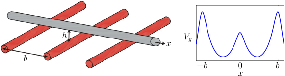
Figure 1: An InAs nanowire (light gray) placed above three gold electrodes. The three electrodes are used to define electrostatically a double quantum dot along the InAs nanowire. A representative curve for the electrostatic potential $V_{g}(x)$ along the wire is shown on the inset to the right. The gold electrodes are placed at positions $x=-b,0,b$, respectively. Typical length scales are $h\simeq 25$ nm and $b\simeq 200$ nm. In the experiment of Ref. [7] two additional gold electrodes were used as plunger gates (not shown).

The choice of material is interesting due to the strong SO coupling and the large $g$-factor in InAs compared to GaAs. In Ref. [8] measurements of a positive correction to the conductivity of InAs nanowires were attributed to weak antilocalization arising from spin relaxation of electrons propagating through the nanowires. This interpretation was supported further by applying a magnetic field that was sufficiently strong to break time-reversal symmetry, thereby suppressing the weak antilocalization correction to the conductivity. A spin relaxation length on the order of 200 nm was reported, but no definitive microscopic theory for the underlying spin-orbit coupling mechanism could be given. The exact nature of the SO coupling in InAs nanowires is still to be fully understood and deserves further experimental and theoretical investigation. We expect, however, that the allowed type and strength of the SO coupling in InAs nanowires are highly dependent on various experimentally controllable parameters, e.g., the growth direction of the nanowire.

3 Single-spin manipulation

We now describe how the SO coupling can be used to flip the spin of an electron in a controllable manner. Motivated by the structure described above we consider a one-dimensional system consisting of a single electron trapped in a gate-defined quantum dot which we approximate with the harmonic potential $V(x,t)=\frac{1}{2}m\omega_{0}^{2}(x-\bar{x}(t))^{2}$ along the $x$-axis. We assume that the minimum position of the harmonic potential, denoted $\bar{x}(t)$, can be varied by changing the voltages on the gate electrodes. A static $B$-field perpendicular to the $x$-axis splits the spin states and determines the $z$-axis. The $x$-, $y$-, and $z$-axis define the lab frame in which the Hamiltonian reads

$$H_{\mathrm{lab}}=\frac{p_{x}^{2}}{2m}+\frac{1}{2}m\omega_{0}^{2}(x-\bar{x}(t))^{2}+\frac{1}{2}g\mu_{B}B\sigma_{z}+\alpha p_{x}\sigma_{y}.$$ (1)

Here $\alpha$ denotes the strength of the SO coupling. The particular form of the SO coupling is assumed to arise from lack of inversion symmetry in the $yz$-plane [9]. In order to get a feeling for the SO coupling it is useful to introduce the SO length $l_{\mathrm{so}}\equiv\hbar/m\alpha$: Without an applied $B$-field, a spin along the $z$-axis is flipped after having traveled the distance $\pi\l_{\mathrm{so}}/2$ along the $x$-axis. Another important length scale is the oscillator length defined as $l_{0}\equiv\sqrt{\hbar/m\omega_{0}}$.

It is convenient to work in a frame that follows the SO induced rotation of the spin. We shall refer to this frame as the rest frame. The Hamiltonian in the rest frame $H_{\mathrm{rest}}$ is obtained by the unitary transformation $H_{\mathrm{rest}}=UH_{\mathrm{lab}}U^{\dagger}$, where $U=\exp{(i\sigma_{y}(x-\bar{x}(0))/l_{\mathrm{so}})}$, and we find

$$H_{\mathrm{rest}}=\frac{p_{x}^{2}}{2m}+\frac{1}{2}m\omega_{0}^{2}(x-\bar{x}(t))^{2}+\frac{1}{2}g\mu_{B}B\left[\cos{\left(\frac{2(x-\bar{x}(0))}{l_{\mathrm{so}}}\right)}\sigma_{z}-\sin{\left(\frac{2(x-\bar{x}(0))}{l_{\mathrm{so}}}\right)}\sigma_{x}\right].$$ (2)

The static $B$-field in the lab frame is rotating in the rest frame of the spin as it travels along the $x$-axis. In the following we work in a regime, where the equilibrium position $\bar{x}(t)$ is slowly changed on the time-scale of the orbital degree of freedom, while fast on the time-scale of the spin, i.e., $g\mu_{B}B/\hbar\ll(1/l_{0})d\bar{x}(t)/dt\ll\omega_{0}$. This allows us to trace out the orbital degree of freedom by projecting $H_{\mathrm{rest}}$ onto the oscillator ground state, whereby we arrive at an effective spin Hamiltonian reading

$$H_{\mathrm{spin}}=\frac{1}{2}\tilde{g}\mu_{B}B\left[\cos{\left(\frac{2(\bar{x}(t)-\bar{x}(0))}{l_{\mathrm{so}}}\right)}\sigma_{z}-\sin{\left(\frac{2(\bar{x}(t)-\bar{x}(0))}{l_{\mathrm{so}}}\right)}\sigma_{x}\right]$$ (3)

with the renormalized $g$-factor given by

$$\tilde{g}=g\left\langle e^{2i(x-\bar{x}(0))/\l_{\mathrm{so}}}\right\rangle=ge^{-(\l_{0}/\l_{\mathrm{so}})^{2}}.$$ (4)

Here the brackets denote an average with respect to the oscillator ground state.

Using the spin Hamiltonian given in Eq. (4) we can manipulate the spin by changing the equilibrium position $\bar{x}(t)$. Below we describe a scheme for spin flips, which does not rely on any resonance conditions as in previous studies [10, 11]. Instead, our scheme relies on fast (on the time scale of the spin) and large (on the order of $l_{\mathrm{so}}$) changes of $\bar{x}(t)$ obtained by controlling the potentials on the gate electrodes. Considering a spin being in an eigenstate of the spin Hamiltonian at $t=0$, i.e., $H_{\mathrm{spin}}=\frac{1}{2}\tilde{g}\mu_{B}B\sigma_{z}$, the scheme reads:

1. Fast displacement of $\bar{x}(t)$: $\bar{x}(0)\rightarrow\bar{x}(0)+\pi l_{\mathrm{so}}/4$. This rotates the $B$-field into the $x$-axis of the rest frame.

2. Free evolution of the spin now governed by the spin Hamiltonian $H_{\mathrm{spin}}=-\frac{1}{2}\tilde{g}\mu_{B}B\sigma_{x}$ for a time span $\Delta t=\hbar\pi/\tilde{g}\mu_{B}B$. This rotates the spin in the rest frame by $\pi$ around the $x$-axis.

3. Fast return of $\bar{x}(t)$: $\bar{x}(0)+\pi l_{\mathrm{so}}/4\rightarrow\bar{x}(0)$. This returns the $B$-field to the initial position in the rest frame, pointing along the $z$-axis.

After the three steps, a spin initially prepared in an eigenstate of $H_{\mathrm{spin}}=\frac{1}{2}\tilde{g}\mu_{B}B\sigma_{z}$ has been flipped into the other eigenstate. For realistic experimental parameters one finds an estimated time for the spin flip process on the order of 0.1 ns [5]. A graphical interpretation of the spin flip process (as seen in the lab frame) is given in Fig. 2. We note that the spin Hamiltonian given in Eq. (4) allows for rotations of the spin to any point on the Bloch sphere.

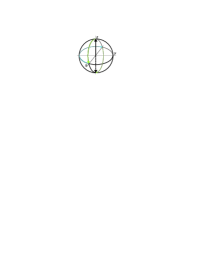
Figure 2: Bloch sphere in the lab frame with the full black arrow denoting the initial spin state. The three colored dashed lines indicate the rotations of the spin during the spin flip scheme. The green lines correspond to the fast displacements of $\bar{x}(t)$, while the blue line in the $xy$-plane corresponds to the rotation around the static $B$-field. The dashed black arrow denotes the final spin state.

4 Two-spin manipulation

The SO coupling also couples spins in neighboring quantum dots. The form and the strength of the coupling can be found by considering two electrons, each described by a (rest frame) Hamiltonian $H^{(i)}_{\mathrm{rest}}$ of the form given in Eq. (2) with different values of $\bar{x}_{i}$, $i=1,2$, for each of the two quantum dots. The orbital degrees of freedom are coupled due to the Coulomb interaction between the electrons, which we expand using $1/|x_{2}-x_{1}|\simeq 1/d-\delta/d^{2}+\delta^{2}/d^{3}$, where we have introduced the distance between the quantum dots $d\equiv\bar{x}_{2}-\bar{x}_{1}>0$ and assumed that $d\gg\delta\equiv(x_{2}-\bar{x}_{2})-(x_{1}-\bar{x}_{1})$. Retaining only the term in the expansion of the Coulomb interaction that couples the positions of the electrons, the two-particle Hamiltonian reads

$$H=H^{(1)}_{\mathrm{rest}}+H^{(2)}_{\mathrm{rest}}-\frac{e^{2}}{2\pi\varepsilon_{0}\varepsilon_{r}d^{3}}(x_{1}-\bar{x}_{1})(x_{2}-\bar{x}_{2}).$$ (5)

For the two-spin coupling temporal variations of $\bar{x}_{i},$ $i=1,2,$ are not necessary.

An effective two-spin Hamiltonian $H_{\mathrm{eff}}$ can be found using imaginary time formalism. The two-particle Hamiltonian given in Eq. (5) is written $H=H_{0}+H^{\prime}$, where $H_{0}$ denotes the Hamiltonian of the two oscillators and $H^{\prime}\equiv H-H_{0}$. We define $e^{-\beta H_{\mathrm{eff}}}\equiv\mathrm{Tr_{osc}}(e^{-\beta H})/Z_{0}$, $Z_{0}\equiv\mathrm{Tr_{osc}}(e^{-\beta H_{0}})$, where $\mathrm{Tr_{osc}}$ denotes a (partial) trace over the two oscillators. Introducing the operator $\hat{U}(\beta)\equiv e^{\beta H_{0}}e^{-\beta H}$, and the thermal average of an operator $A$ with respect to $H_{0}$, $\langle A\rangle_{0}\equiv\mathrm{Tr_{osc}}(Ae^{-\beta H_{0}})/Z_{0}$, we write $e^{-\beta H_{\mathrm{eff}}}=\langle\hat{U}(\beta)\rangle_{0}$. Using the formal expression $\hat{U}(\beta)=T_{\tau}\exp\left(-\int_{0}^{\beta}d\tau\hat{H}^{\prime}(\tau)\right)$, where $T_{\tau}$ denotes the (imaginary) time-ordering operator and $\hat{H}^{\prime}(\tau)\equiv e^{\tau H_{0}/\hbar}H^{\prime}e^{-\tau H_{0}/\hbar}$ is the interaction picture representation of $H^{\prime}$ (in imaginary time), we can in principle calculate the effective two-spin Hamiltonian $H_{\mathrm{eff}}$ to any order in $H^{\prime}$. The first non-vanishing term that couples the two spins arises from the expansion of $\hat{U}(\beta)$ to third order in $H^{\prime}$ and has the form $\tau_{xx}\sigma_{x}^{(1)}\sigma_{x}^{(2)}$, where $\tau_{xx}$ is to be determined. Concentrating on this term, we find

$$e^{-\beta H_{\mathrm{eff}}}\simeq\ldots+\frac{(eg\mu_{B}B)^{2}}{8\pi\varepsilon_{0}\varepsilon_{r}d^{3}}\int_{0}^{\beta}\int_{0}^{\beta}\int_{0}^{\beta}d\tau_{1}d\tau_{2}d\tau_{3}\mathcal{G}(x_{1}-\bar{x}_{1},\tau_{1}-\tau_{2})\mathcal{G}(x_{2}-\bar{x}_{2},\tau_{2}-\tau_{3})\sigma_{x}^{(1)}\sigma_{x}^{(2)}+\ldots,$$ (6)

where we have assumed that the spin degrees of freedom evolve much slower than the orbital part, and $\hat{\sigma}_{x}^{(1)}$ and $\hat{\sigma}_{x}^{(2)}$ are thus taken to be time-independent. The correlation function $\mathcal{G}(x_{i},\tau)$ is defined as

$$\mathcal{G}(x_{i},\tau)\equiv\left\langle T_{\tau}\sin\left(\frac{2\hat{x}_{i}(\tau)}{l_{\mathrm{so}}}\right)x_{i}\right\rangle_{0},$$ (7)

and can be evaluated using linked cluster theory. We find

$$\mathcal{G}(x_{i},\tau)=\frac{l_{0}^{2}}{l_{\mathrm{so}}}e^{-(l_{0}/l_{\mathrm{so}})^{2}}\Big{[}\Theta(\tau)\Big{(}n_{B}(\beta\hbar\omega_{0})e^{\omega_{0}\tau}+(1+n_{B}(\beta\hbar\omega_{0}))e^{-\omega_{0}\tau}\Big{)}+(\tau\rightarrow-\tau)\Big{]},$$ (8)

where $\Theta(\tau)$ is the Heaviside step function and $n_{B}(x)=1/(e^{x}-1)$. Collecting all terms and carrying out the triple integral, we find

$$e^{-\beta H_{\mathrm{eff}}}=\ldots+\frac{e^{2}}{4\pi\varepsilon_{0}\varepsilon_{r}}\frac{2\l_{0}^{4}(g\mu_{B}B)^{2}}{\l_{\mathrm{so}}^{2}(\hbar\omega_{0})^{3}d^{3}}e^{-2(l_{\mathrm{so}}/l_{0})^{2}(1+n_{B}(\beta\hbar\omega_{0}))}F(\beta\hbar\omega_{0})\sigma_{x}^{(1)}\sigma_{x}^{(2)}+\ldots$$ (9)

with $F(x)=[x(\cosh(x)-2)+\sinh(x)]/2\sinh^{2}(x/2)$. Having solved the finite-temperature ($\beta<\infty$) problem, we let $\beta\rightarrow\infty$, and identify

$$\tau_{xx}=-\frac{e^{2}}{4\pi\varepsilon_{0}\varepsilon_{r}}\frac{2\l_{0}^{4}(\tilde{g}\mu_{B}B)^{2}}{\l_{\mathrm{so}}^{2}(\hbar\omega_{0})^{2}d^{3}}$$ (10)

in agreement with our previous work [5]. The imaginary time formalism outlined here allows for calculation of the coupling to higher order in the Coulomb interaction and corrections due to a finite temperature.

5 Numerics

In Ref. [5] we used a numerical implementation of the two-particle Hamiltonian in Eq. (5) to study the coupling $\tau_{xx}$ in case of non-harmonic confining potentials. Here we use the numerical implementation to calculate $\tau$ as a function of the SO coupling strength $\alpha$. In Fig. 3 we show a comparison of numerical results for $\tau_{xx}$ using nearly harmonic confining potentials and Eq. (10). The numerical results agree well with the analytic results, and as expected the coupling depends quadratically on $\alpha$, i.e., $\tau_{xx}\propto\alpha^{2}$ for small values of $\alpha$ (corresponding to $l_{\mathrm{so}}\gg l_{0}$), while it for large values of $\alpha$ is dominated by the renormalized $g$-factor which drops off exponentially with increasing $\alpha$.

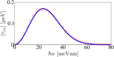
Figure 3: Two-qubit coupling $\tau_{xx}$ as a function of the SO coupling $\alpha$. Parameters are $\varepsilon_{r}=15.15$, $m=0.027m_{e}$, $g=14.8$, $B=160$ mT, $l_{0}=80$ nm ($\hbar\omega_{0}\simeq 0.4$ meV) and $d\simeq 0.75$ $\mu$m. Circles indicate numerical results, while the full line shows Eq. $(\ref{eq_tau})$.

6 Conclusion

We have elaborated on our recent proposal for spin-qubit manipulation using the SO coupling in nanostructures. We have discussed an experimental setup with strong SO coupling which may be relevant for realizing our proposal. We have described in detail how single-spin rotations may be carried out using fast displacements of the electron(s), and we have derived an expression for the effective two-spin interaction using imaginary-time formalism. Finally, we have shown that the analytic result for the two-spin interaction agrees with numerics.

The authors thank G Burkard, X Cartoixa, W A Coish, A Fuhrer and J M Taylor for illuminating discussions during the preparation of this manuscript.

References

References

- [1] Loss D and DiVincenzo D P 1998 Phys. Rev. A 57 120
- [2] Burkard G, Loss D and DiVincenzo D P 1999 Phys. Rev. B 59 2070
- [3] Petta J R et al. 2005 Science 309 2180
- [4] Coish W A and Loss D 2006 cond-mat/0606550
- [5] Flindt C, Sørensen A S and Flensberg K 2006 cond-mat/0603559
- [6] Hu X and Das Sarma S 2006 Phys. Rev. Lett. 96 100501
- [7] Fasth C, Fuhrer A, Björk M T and Samuelson L 2005 Nano Lett. 5 1487
- [8] Hansen A E et al. 2005 Phys. Rev. B 71 205328
- [9] Levitov L S and Rashba E I 2003 Phys. Rev. B 67 115324
- [10] Rashba E I and Efros A L 2003 Phys. Rev. Lett. 91 126405
- [11] Golovach V N, Borhani M and Loss D 2006 cond-mat/0601674