Dephasing in the semiclassical limit is system–dependent

Abstract

We investigate dephasing in open quantum chaotic systems in the limit of large system size to Fermi wavelength ratio, $L/\lambda_{\rm F}\gg 1$. We semiclassically calculate the weak localization correction $g^{\rm wl}$ to the conductance for a quantum dot coupled to (i) an external closed dot and (ii) a dephasing voltage probe. In addition to the universal algebraic suppression $g^{\rm wl}\propto(1+\tau_{\rm D}/\tau_{\phi})^{-1}$ with the dwell time $\tau_{\rm D}$ through the cavity and the dephasing rate $\tau_{\phi}^{-1}$, we find an exponential suppression of weak localization by a factor $\propto\exp[-\tilde{\tau}/\tau_{\phi}]$, with a system-dependent $\tilde{\tau}$. In the dephasing probe model, $\tilde{\tau}$ coincides with the Ehrenfest time, $\tilde{\tau}\propto\ln[L/\lambda_{\rm F}]$, for both perfectly and partially transparent dot-lead couplings. In contrast, when dephasing occurs due to the coupling to an external dot, $\tilde{\tau}\propto\ln[L/\xi]$ depends on the correlation length $\xi$ of the coupling potential instead of $\lambda_{\rm F}$.

Introduction. Electronic transport in mesoscopic systems exhibits a range of quantum coherent effects such as weak localization, universal conductance fluctuations and Aharonov-Bohm effects Sto92 ; Imr97 . Being intermediate in size between micro- and macroscopic systems, these systems are ideal playgrounds to investigate the quantum-to-classical transition from a microscopic coherent world, where quantum interference effects prevail, to a macroscopic classical world Joo03 . Indeed, the disappearance of quantum coherence in mesoscopic systems as dephasing processes set in has been the subject of intensive theoretical Alt82 ; But86 ; Bar99 ; dephasing and experimental  Hui98 ; Han01 ; Pie03 studies. When the temperature is sufficiently low, it is accepted that the dominant processes of dephasing are electronic interactions. In disordered systems, dephasing due to electron-electron interactions is known to be well modeled by a classical noise potential Alt82 , which gives an algebraic suppression of the weak localization correction to conductance through a diffusive quantum dot,

$$g^{\rm wl}=g_{0}^{\rm wl}\big{/}(1+\tau_{\rm D}/\tau_{\phi}).$$ (1)

Here, $g_{0}^{\rm wl}$ is the weak localization correction (in units of $2e^{2}/h$) without dephasing, the dephasing time $\tau_{\phi}$ is given by the noise power, and $\tau_{\rm D}$ is the electronic dwell time in the dot. Eq. (1) is insensitive to most noise-spectrum details, and holds for other noise sources such as electron-phonon interactions or external microwave fields.

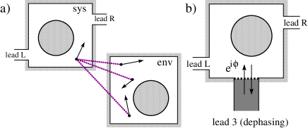
Figure 1: a) (left panel) Schematic of the system-environment model. The system is an open quantum dot that is coupled to an environment in the shape of a second, closed quantum dot. b) (right panel) Schematic of the dephasing lead model.

Other, mostly phenomenological models of dephasing have been proposed to study dephasing in ballistic systems But86 ; dephasing ; Bar99 , the most popular of which, perhaps, being the dephasing lead model But86 ; Bar99 . A cavity is connected to two external, L (left) and R (right) leads of widths $W_{\rm L},W_{\rm R}$. A third lead of width $W_{3}$ is connected to the system via a tunnel-barrier of transparency $\rho$. A voltage is applied to the third lead to ensure that no current flows through it on average. A random matrix theory (RMT) treatment of the dephasing lead model leads to Eq. (1) with $\tau_{\rm D}=\tau_{0}L/(W_{\rm L}+W_{\rm R})$ and $\tau_{\phi}=\tau_{0}L/(\rho W_{3})$, in term of the dot’s time of flight $\tau_{0}$ Bar99 ; Ben97 . Thus it is commonly assumed that dephasing is system-independent. The dephasing lead model is often used phenomenologically in contexts where the source of dephasing is unknown.

Our purpose in this article is to revisit dephasing in open chaotic ballistic systems with a focus on whether dephasing remains system-independent in the semiclassical limit of large ratio $L/\lambda_{\rm F}$ of the system size to Fermi wavelength. This regime sees the emergence of a finite Ehrenfest time scale, $\tau_{\rm E}^{\rm cl}=\lambda^{-1}\ln[L/\lambda_{\rm F}]$ ($\lambda$ is the Lyapunov exponent), in which case dephasing can lead to an exponential suppression of weak localization, $\propto\exp[-\tau_{\rm E}^{\rm cl}/\tau_{\phi}]\big{/}(1+\tau_{\rm D}/\tau_{\phi})$ Ale96 . Subsequent numerical investigations on the dephasing lead model support this prediction Two04 . Here we analytically investigate two different models of dephasing, and show that the suppression of weak localization is strongly system-dependent. First, we construct a new formalism that incorporates the coupling to external degrees of freedom into the scattering approach to transport. This approach is illustrated by a semiclassical calculation of weak localization in the case of an environment modeled by a capacitively coupled, closed quantum dot. We restrict ourselves to the regime of pure dephasing, where the environment does not alter the classical dynamics of the system. Second, we provide the first semiclassical treatment of transport in the dephasing lead model. We show that in both cases, the weak localization correction to conductance is

$$g^{\rm wl}=g^{\rm wl}_{0}\;\exp[-\tilde{\tau}/\tau_{\phi}]\;\big{/}(1+\tau_{\rm D}/\tau_{\phi}),$$ (2)

where $g^{\rm wl}_{0}$ is the finite-$\tau_{\rm E}^{\rm cl}$ correction in absence of dephasing. The time scale $\tilde{\tau}$ is system-dependent. For the dephasing lead model, $\tilde{\tau}=\tau_{\rm E}^{\rm cl}+(1-\rho)\tau_{\rm E}^{\rm op}$ in terms of the transparency $\rho$ of the contacts to the leads, and the open system Ehrenfest time $\tau_{\rm E}^{\rm op}=\lambda^{-1}\ln[W^{2}/\lambda_{\rm F}L]$. This analytic result fits the numerics of Ref. Two04 , and (up to logarithmic corrections) is in agreement with Ref. Ale96 . Yet for the system-environment model, $\tilde{\tau}=\lambda^{-1}\ln[(L/\xi)^{2}]$ depends on the correlation length $\xi$ of the inter-dot coupling potential. We thus conclude that dephasing in the semiclassical limit is system-dependent.

Transport theory for a system-environment model. In the standard theory of decoherence, one starts with the total density matrix $\eta_{\rm tot}$ including both system and environment degrees of freedom Joo03 . The time-evolution of $\eta_{\rm tot}$ is unitary. The observed properties of the system alone are given by the reduced density matrix $\eta_{\rm sys}$, obtained by tracing $\eta_{\rm tot}$ over the environment degrees of freedom. This is probability conserving, ${\rm Tr}\;\eta_{\rm sys}=1$, but renders the time-evolution of $\eta_{\rm sys}$ non-unitary. The decoherence time is inferred from the decay rate of its off-diagonal matrix elements Joo03 . We generalize this approach to the scattering theory of transport.

To this end, we consider two coupled chaotic cavities as sketched in Fig. 1a. Few-electron double-dot systems similar to the one considered here have recently been the focus of intense experimental efforts Wiel03 . One of them (the system) is an open quantum dot connected to two external leads. The other one (the environment) is a closed quantum dot, which we model using RMT. The two dots are chaotic and capacitively coupled. In particular, they do not exchange particles. We require that $\lambda_{\rm F}\ll W_{\rm L,R}\ll L$, so that the number of transport channels satisfies $1\ll N_{\rm L,\,R}\ll L/\lambda_{F}$ and the chaotic dynamics inside the dot has enough time to develop, $\lambda\tau_{\rm D}\gg 1$. Electrons in the leads do not interact with the second dot. Inside each cavity the dynamics is generated by chaotic Hamiltonians $H_{\rm sys}$ and $H_{\rm env}$. We only specify that the capacitative coupling potential, ${\cal U}$, is smooth, and has magnitude $U$ and correlation length $\xi$.

The environment coupling can be straightforwardly included in the scattering approach, by writing the scattering matrix, ${\mathbb{S}}$, as an integral over time-evolution operators. We then use a bipartite semiclassical propagator to write the matrix elements of ${\mathbb{S}}$ for given initial and final environment positions, $({\bf q}_{0},{\bf q})$, as

$${\mathbb{S}}_{\rm mn}({\bf q}_{0},{\bf q}) = (2\pi)^{-1}\int_{0}^{\infty}\!{\rm d}t\!\int_{\rm L}\!{\rm d}{\bf y}_{\rm 0}\!\int_{\rm R}\!{\rm d}{\bf y}\,\left\langle m|{\bf y}\right\rangle\left\langle{\bf y}_{\rm 0}|n\right\rangle\,$$ (3)

$$\times \sum_{\gamma,\Gamma}(C_{\gamma}\;C_{\Gamma})^{\frac{1}{2}}\exp[{\it i}\left\{S_{\gamma}+S_{\Gamma}+{\cal S}_{\gamma,\Gamma}\right\}].\quad$$

This is a double sum over classical paths, labeled $\gamma$ for the system and $\Gamma$ for the environment. For pure dephasing, the classical path $\gamma$ ($\Gamma$) connecting ${\bf y_{0}}$ (${\bf q_{0}}$) to ${\bf y}$ (${\bf q}$) in the time $t$ is solely determined by $H_{\rm sys}$ ($H_{\rm env}$). The prefactor $C_{\gamma}C_{\Gamma}$ is the inverse determinant of the stability matrix, and the exponent contains the non-interacting action integrals, $S_{\gamma},S_{\Gamma}$, accumulated along $\gamma$ and $\Gamma$, and the interaction term, ${\cal S}_{\gamma,\Gamma}=\int_{0}^{t}\!{\rm d}\tau{\cal U}[{\bf y}_{\gamma}(\tau),{\bf q}_{\Gamma}(\tau)]$.

Since we assume that particles in the leads do not interact with the second cavity, we can write the initial total density matrix as $\eta^{(n)}=\eta_{\rm sys}^{(n)}\otimes\eta_{\rm env}$, with $\eta_{\rm sys}^{(n)}=|n\rangle\langle n|$, $n=1,2,...N_{\rm L}$. We take $\eta_{\rm env}$ as a random matrix, though our approach is not restricted to that particular choice. We define the conductance matrix as the following trace over the environment degrees of freedom,

$$g_{mn}^{(r)}=\big{\langle}m\big{|}{\rm Tr}_{\rm env}\big{[}{\mathbb{S}}\;\eta^{(n)}\;{\mathbb{S}}^{\dagger}\big{]}\big{|}m\big{\rangle}.$$ (4)

The conductance is then given by $g=\sum_{m,n}g_{mn}^{(r)}$. This construction is current conserving, however the environment-coupling generates decoherence and the suppression of coherent contributions to transport. To see this we now calculate the conductance to leading order in the weak localization correction.

We insert Eq. (3) into Eq. (4), perform the sum over channel indices with the semiclassical approximation $\sum_{n}^{N_{\rm L}}\langle{\bf y}_{0}|n\rangle\langle n|{\bf y}^{\prime}_{0}\rangle\approx\delta({\bf y}^{\prime}_{0}-{\bf y}_{0})$ Jac06 , and use the RMT result $\overline{\langle{\bf q}_{0}|\eta_{\rm env}|{\bf q}_{0}^{\prime}\rangle}\approx\Omega_{\rm env}^{-1}\delta({\bf q}_{0}^{\prime}-{\bf q}_{0})$, where $\Omega_{\rm env}$ is the environment volume caveat0 . The conductance then reads

$$g = \left(4\pi^{2}\,\Omega_{\rm env}\right)^{-1}\int_{0}^{\infty}\!\!{\rm d}t\;{\rm d}t^{\prime}\int_{\rm\Omega_{env}}\!\!{\rm d}{\bf q}_{0}\;{\rm d}{\bf q}\int_{\rm L}\!\!{\rm d}{\bf y}_{0}\int_{\rm R}\!{\rm d}{\bf y}$$ (5)

$$\times \sum_{\gamma,\Gamma;\gamma^{\prime},\Gamma^{\prime}}\left(C_{\gamma}\;C_{\Gamma}\;C_{\gamma^{\prime}}\;C_{\Gamma^{\prime}}\right)^{\frac{1}{2}}\;\;e^{i(\Phi_{\rm sys}+\Phi_{\rm env}+\Phi_{\cal U})}.\qquad$$

This is a quadruple sum over classical paths of the system ($\gamma$ and $\gamma^{\prime}$, going from ${\bf y}_{0}$ to ${\bf y}$) and the environment ($\Gamma$ and $\Gamma^{\prime}$, going from ${\bf q}_{0}$ to ${\bf q}$), with action phases $\Phi_{\rm sys}=S_{\gamma}({\bf y}_{0},{\bf y};t)-S_{\gamma^{\prime}}({\bf y}_{0},{\bf y};t^{\prime})$, $\Phi_{\rm env}=S_{\Gamma}({\bf q}_{0},{\bf q};t)-S_{\Gamma^{\prime}}({\bf q}_{0},{\bf q};t^{\prime})$ and $\Phi_{\cal U}={\cal S}_{\gamma,\Gamma}({\bf y}_{0},{\bf y};{\bf q}_{0},{\bf q};t)-{\cal S}_{\gamma^{\prime},\Gamma^{\prime}}({\bf y}_{0},{\bf y};{\bf q}_{0},{\bf q};t^{\prime})$. We are interested in the conductance averaged over energy variations, and hence look for contributions to Eq. (5) with stationary $\Phi_{\rm sys},\Phi_{\rm env}$. The first such contributions are the diagonal ones with $\gamma=\gamma^{\prime}$ and $\Gamma=\Gamma^{\prime}$, for which $\Phi_{\cal U}=0$. They are ${\cal U}$-independent and give the classical, Drude conductance, $g^{\rm D}=N_{\rm L}N_{\rm R}/(N_{\rm L}+N_{\rm R})$. The leading order correction to this comes from weak-localization paths $\gamma$ and $\gamma^{\prime}$ Ale96 ; wl_semicl ; Jac06 ; Bro06-cbs (see Fig. 2), with $\Gamma^{\prime}=\Gamma$ for environment paths caveat1 . In the absence of dephasing these contributions accumulate a phase difference $\delta\Phi_{\rm sys}$. Semiclassically these contributions give $g_{0}^{\rm wl}=-\exp[-\tau_{\rm E}^{\rm cl}/\tau_{\rm D}]\;N_{\rm L}N_{\rm R}/(N_{\rm L}+N_{\rm R})^{2}$ wl_semicl ; Jac06 ; Bro06-cbs .

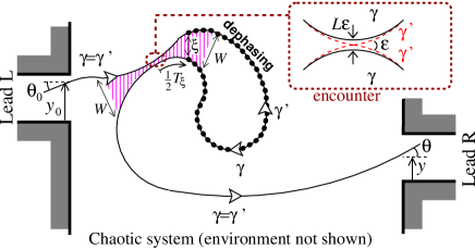
Figure 2: (color online) A semiclassical contribution to weak localization for the system-environment model. The paths are paired everywhere except at the encounter. There one crosses itself at angle $\epsilon$, while the other does not (going the opposite way around the loop). Here we show $\xi>\epsilon L$, so the dephasing (dotted path segment) starts in the loop ($T_{\xi}>0$).

In the presence of an environment, each weak localization pair of paths accumulates an additional action phase difference $\delta\Phi_{\cal U}$, which is averaged over. Dephasing occurs mostly in the loop, when the paths are more than the correlation length $\xi$ apart (see Fig. 2). Thus we can define $T_{\xi}=\lambda^{-1}\ln[(\xi/\epsilon L)^{2}]$ as twice the time between the encounter and the start of dephasing. If $\xi<\epsilon L$, dephasing starts before the paths reach the encounter, $T_{\xi}<0$ caveat2 . Using the central limit theorem and assuming a fast decaying interaction correlator, $\left\langle{\cal U}[{\bf y}_{\gamma}(\tau),{\bf q}_{\Gamma}(\tau)]{\cal U}[{\bf y}_{\gamma}(\tau^{\prime}),{\bf q}_{\Gamma}(\tau^{\prime})]\right\rangle_{\Gamma}$$\,\propto\,$$\tau_{\phi}^{-1}\exp[-\{{\bf y}_{\gamma}(\tau)-{\bf y}_{\gamma}(\tau^{\prime})\}/\xi]$, the average phase difference due to ${\cal U}$ reads

$$\big{\langle}e^{{\it i}\delta\Phi_{\cal U}}\big{\rangle}=e^{-\frac{1}{2}\langle\delta\Phi^{2}_{\cal U}\rangle}=\exp\left[-(t_{2}-t_{1}-T_{\xi})/\tau_{\phi}\right],$$ (6)

where $t_{1}$ ($t_{2}$) gives the start (end) of the loop. The derivation then proceeds as for ${\cal U}=0$ Jac06 , except that during the time $(t_{2}-t_{1}-T_{\xi})$, the dwell time is effectively divided by $[1+\tau_{\rm D}/\tau_{\phi}]$, so the $(t_{2}-t_{1})$-integral generates an extra prefactor of $[1+\tau_{\rm D}/\tau_{\phi}]^{-1}\exp[-\tau_{\xi}/\tau_{\phi}]$ where $\tau_{\xi}=\lambda^{-1}\ln[(L/\xi)^{2}]$. Thus the weak localization correction is as in Eq. (2) with $\tilde{\tau}$ given by $\tau_{\xi}$. In contrast to Ref. Ale96 , the exponent depends on $\xi$ not $\lambda_{\rm F}$.

A calculation of coherent-backscattering with dephasing to be presented elsewhere enables us to show that our approach is probability- and thus current-conserving. We also point out that (for $\tau_{\phi}\sim\tau_{D}$) one can ignore the modifications of the classical paths due to the coupling to the environment, as long as $\xi\gg[\lambda_{\rm F}L/\lambda\tau_{D}]^{1/2}$. Thus our method is applicable for $\xi$ smaller (as well as larger) than the encounter size $[\lambda_{\rm F}L]^{1/2}$, but not for $\xi\sim\lambda_{\rm F}$.

Dephasing lead model. We next add a third lead to an otherwise closed dot (as in Fig. 1b), and tune the potential on this lead such that the net current through it is zero. Thus every electron that leaves through lead 3 is replaced by one with an unrelated phase, leading to a loss of phase information without loss of particles. In this situation the conductance from L to R is given by $g=T_{\rm LR}+T_{\rm L3}\,T_{\rm R3}\;(T_{\rm L3}+T_{\rm R3})^{-1}$ But86 , where $T_{nm}$ is the conductance from lead $m$ to lead $n$ when we do not tune the potential on lead $3$ to ensure zero current. We next note that $T_{nm}=T_{nm}^{\rm D}+\delta T_{nm}+{\cal O}[N^{-1}]$ where the Drude contribution, $T_{nm}^{\rm D}$, is ${\cal O}[N]$ and the weak localization contribution, $\delta T_{nm}$, is ${\cal O}[1]$. If we now expand $g$ for large $N$ and collect all ${\cal O}[1]$-terms we get

$$g^{\rm wl}=\delta T_{\rm LR}+\frac{(T^{\rm D}_{\rm L3})^{2}\;\delta T_{\rm R3}+(T^{\rm D}_{\rm R3})^{2}\;\delta T_{\rm L3}}{(T^{\rm D}_{\rm L3}+T^{\rm D}_{\rm R3})^{2}}.$$ (7)

For a cavity perfectly connected to all three leads (with $W_{L,R,3}\gg\lambda_{\rm F}$), the Drude and weak localization results for ${\cal U}=0$ (at finite-$\tau_{\rm E}^{\rm cl}$)  Jac06 can be substituted into Eq. (7), immediately giving Eq. (2) with $\tilde{\tau}$ given by $\tau_{\rm E}^{\rm cl}$.

To connect with the numerics of Ref. Two04 , we now consider a tunnel-barrier with finite transparency $0\leq\rho_{3}\leq 1$ between the cavity and the dephasing lead. Introducing tunnel-barriers into the trajectory-based theory of weak localization is detailed in Ref. Whi06 . It requires three main changes to the theory in Ref. Jac06 . (i) The dwell time (single path survival time) becomes $\tau_{\rm D1}^{-1}=(\tau_{0}L)^{-1}\sum_{m}\rho_{m}W_{m}$. (ii) The paired path survival time (for two paths closer than the lead width) is no longer equal to the dwell time, instead it is $\tau_{\rm D2}^{-1}=(\tau_{0}L)^{-1}\sum_{m}\rho_{m}(2-\rho_{m})W_{m}$ because survival requires that both paths hitting a tunnel-barrier are reflected Whi06 . (iii) The coherent-backscattering peak contributes to transmission as well as reflection, see Fig. 3.

For the Drude conductance we need only (i) above, giving us $T^{\rm D}_{nm}=\rho_{m}\;\rho_{n}N_{m}N_{n}/{\mathcal{N}}$, where ${\mathcal{N}}=\sum_{k}\rho_{k}N_{k}$. For the conventional weak localization correction we need (i) and (ii). The contribution’s classical path stays within $W$ of itself for a time $T_{W}(\epsilon)/2$ on either side of the encounter (dashed region in Figs. 2 and 3), thus we must use the paired-paths survival time, $\tau_{\rm D2}$, for these parts of the path. Elsewhere the survival time is given by $\tau_{\rm D1}$. We follow the derivation in Ref. Jac06 with these new ingredients, and the conventional weak localization correction becomes $\delta T^{(0)}_{nm}=-(\rho_{m}\rho_{n}N_{m}N_{n}/{\mathcal{N}}^{2})(\tau_{\rm D1}/\tau_{\rm D2})\exp[-\Theta]$. The exponential with $\Theta=\tau_{\rm E}^{\rm op}/\tau_{\rm D_{2}}+(\tau_{\rm E}^{\rm cl}-\tau_{\rm E}^{\rm op})/\tau_{\rm D_{1}}$, is the probability that the path segments survive a time $\tau_{\rm E}^{\rm op}$ as a pair ($\tau_{\rm E}^{\rm op}/2$ either side of the encounter) and survive an additional time $(\tau_{\rm E}^{\rm cl}-\tau_{\rm E}^{\rm op})$ unpaired (to form a loop of length $\tau_{\rm E}^{\rm cl}$). However, we must include point (iii) above and consider the failed coherent-backscattering, shown in Fig. 3. We perform the backscattering calculation following Ref. Jac06 (see also Bro06-cbs ) but using $\tau_{\rm D2}$ when the paths are closer than $W$ and $\tau_{\rm D1}$ elsewhere. We then multiply the result by the probability that the path reflects off lead $m$ and then escapes through lead $n$. This gives a contribution, $\delta T^{\rm cbs}_{nm}=-(\rho_{m}(1-\rho_{m})\rho_{n}N_{m}N_{n}/{\mathcal{N}}^{2})\exp[-\Theta]$ assuming $n\neq m$. There is a second such contribution with $m\leftrightarrow n$. Summing the contributions for $m\neq n$

$$\delta T_{nm} = (\rho_{m}\rho_{n}N_{m}N_{n}/{\mathcal{N}}^{2})(\rho_{m}+\rho_{n}-\tilde{\mathcal{N}}/{\mathcal{N}}){\rm e}^{-\Theta}\quad$$ (8)

where $\tilde{\mathcal{N}}=\sum_{k}\rho_{k}^{2}N_{k}$. If only the dephasing lead has a tunnel-barrier, substituting the Drude and weak localization results into Eq. (7), we obtain Eq. (2) with $\tilde{\tau}=(1-\rho)\tau_{\rm E}^{\rm op}+\tau_{\rm E}^{\rm cl}$. In this case the exponential in Eq. (2) is the probability that a path does not escape into the dephasing lead in either the paired-region or the extra time $(\tau_{\rm E}^{\rm cl}-\tau_{\rm E}^{\rm op})$ unpaired (for the loop to form).

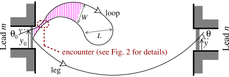
Figure 3: (color online) A failed coherent-backscattering contribution to conductance, $\delta T^{\rm cbs}_{nm}$. It involves paths which return to close but anti-parallel to themselves at lead $m$, but reflects off the tunnel-barrier, remaining in the cavity to finally escape via lead $n$. The cross-hatched region is when the two solid paths are paired (within $W$ of each other).

To generalize our results to $j$ dephasing leads, we expand the relevant conductance formula in powers of $N$ and collect the ${\cal O}[1]$-terms. Then $g^{\rm wl}=\delta T_{\rm LR}+\sum_{m=1}^{j}(A_{m}\delta T_{{\rm L}m}+B_{m}\delta T_{{\rm R}m})$, where the sum is over all dephasing leads. The prefactors $A_{m},B_{m}$ are combinations of Drude conductances and thus independent of $\tau_{\rm E}^{\rm cl},\tau_{\rm E}^{\rm op}$, we need them to get power-law dephasing. However we can already see that there must be exponential decay with $[(1-\rho)\tau_{\rm E}^{\rm op}+\tau_{\rm E}^{\rm cl}]/\tau_{\phi}$, as for $j=1$, where now $\tau_{\phi}^{-1}=(\tau_{0}L)^{-1}\sum_{m}\rho_{m}W_{m}$ and $\rho\tau_{\phi}^{-1}=(\tau_{0}L)^{-1}\sum_{m}\rho_{m}^{2}W_{m}$.

Conclusions. We first observe that the dephasing-lead model has no independent parameter $\xi$. To our surprise it is the Fermi wavelength, not the dephasing-lead’s width, which plays a role similar to $\xi$. Thus a dephasing-lead model cannot mimic a system-environment model with $\xi\sim L$ at finite $\tau_{\rm E}^{\rm cl}$. Our second observation is that Eq. (2) with $\tilde{\tau}=\tau_{\xi}$ is for a regime where ${\cal U}$ does not affect the momentum/energy of classical paths. Therefore, it does not contradict the result with $\tilde{\tau}=\tau_{\rm E}^{\rm cl}$ in Ref. Ale96 , valid for $\xi$ so small that dephasing occurs via a “single inelastic process with large energy transfer” caveat . Intriguingly their result is similar to ours for the dephasing-lead model. Could this be due to the destruction of classical determinism by the dephasing process in both cases?

We finally note that conductance fluctuations (CFs) in the dephasing-lead model exhibit an exponential dependence $\propto\exp[-2\tau_{\rm E}/\tau_{\phi}]$ for $\rho_{3}\ll 1$ Two04 , but recover the universal behavior of Eq. (1) for $\rho_{3}=1$ comment-UCFs . However external noise can lead to dephasing of CFs with a $\tau_{\rm E}$-independent exponential term comment-UCFs , similar to the one found above for weak-localization in the system-environment model. Thus our conclusion, that dephasing is system-dependent in the deep semiclassical limit, also applies to conductance fluctuations.

We thank I. Aleiner, P. Brouwer, M. Büttiker and M. Polianski for useful and stimulating discussions. The Swiss National Science Foundation supported CP, and funded the visits to Geneva of PJ and RW. Part of this work was done at the Aspen Center for Physics.

References

- (1) A.D. Stone in Physics of Nanostructures, J.H. Davies and A.R. Long Eds., Institute of Physics and Physical Society (London, 1992).
- (2) Y. Imry, Introduction to Mesoscopic Physics, Oxford University Press (New York, 1997).
- (3) E. Joos et al., Decoherence and the Appearance of a Classical World in Quantum Theory (Springer, Berlin 2003).
- (4) B.L. Altshuler, A.G. Aronov, and D. Khmelnitsky, J. Phys. C 15, 7367 (1982).
- (5) M. Büttiker, Phys. Rev. B 33, 3020 (1986).
- (6) H.U. Baranger and P.A. Mello, Waves in Random Media 9, 105 (1999).
- (7) M.G. Vavilov and I.L. Aleiner, Phys. Rev. B 60, R16311 (1999). G. Seelig and M. Büttiker, Phys. Rev. B 64, 245313 (2001). M.L. Polianski and P.W. Brouwer, J. Phys. A: Math Gen. 36, 3215 (2003).
- (8) A.G. Huibers et al., Phys. Rev. Lett. 81, 200 (1998).
- (9) A.E. Hansen et al., Phys. Rev. B 64, 045327 (2001); K. Kobayashi, H. Aikawa, S. Katsumoto, and Y. Iye, J. Phys. Soc. Jpn. 71, 2094 (2002).
- (10) F. Pierre et al., Phys. Rev. B 68, 085413 (2003).
- (11) C.W.J. Beenakker, Rev. Mod. Phys. 69, 731 (1997).
- (12) I.L. Aleiner and A.I. Larkin, Phys. Rev. B 54, 14423 (1996).
- (13) J. Tworzydlo et al., Phys. Rev. Lett. 93, 186806 (2004).
- (14) W.G. van der Wiel et al., Rev. Mod. Phys. 75, 1 (2003).
- (15) Ph. Jacquod and R.S. Whitney, Phys. Rev. B 73, 195115 (2006); see in particular section V.
- (16) For a many-particle environment, the coordinate vectors and are -dimensional vectors and where gives the number of particles in the environment, and is its spatial volume.
- (17) K. Richter and M. Sieber, Phys. Rev. Lett. 89, 206801 (2002); I. Adagideli, Phys. Rev. B 68, 233308 (2003); S. Heusler, S. Müller, P. Braun, and F. Haake, Phys. Rev. Lett. 96, 066804 (2006).
- (18) S. Rahav and P.W. Brouwer, Phys. Rev. Lett. 96, 196804 (2006).
- (19) The system’s conductance is unaffected by environment wl contributions, since their integral over is zero.
- (20) Considering a sharp onset of dephasing at is justified by the local exponential instability of classical trajectories and gives the right answer to zeroth order in .
- (21) R.S. Whitney, Phys. Rev. B 75, 235404 (2007).
- (22) Ref. Ale96 mentions that they do not expect their result to hold when is a classical scale.
- (23) A. Altland, P.W. Brouwer, and C. Tian, Phys. Rev. Lett. 99, 036804 (2007) and cond-mat/0605051v1.