Temperature dependence of spin susceptibility in two-dimensional Fermi liquid systems.

Abstract

We consider the non-analytic terms in the spin susceptibility arising as a result of rescaterring of pairs of quasiparticles. We emphasize the importance of rescattering in the Cooper channel for the analysis of the temperature dependences in the two-dimensional electron systems in the ballistic regime. In the calculation of the linear in $T$ term we use angular harmonics in the Cooper channel, because for each harmonic the interaction amplitude is renormalized independently. We observe, that as a consequence of strong renormalizations in the Cooper ladder, the temperature derivative of the spin susceptibility may change its sign at low temperatures.

I Introduction.

Linear in temperature corrections in the spin susceptibility of the two-dimensional (2D) electron gas has been discussed intensively in the past decade.Baranov1993 ; Belitz1996b ; Takahashi1998 ; Misawa1999 ; ChitovLett2001 ; Chubukov2003 ; Galitski2005 ; GlazmanB2005 ; Betouras2005 Our interest to this question is motivated by a recent observation of a strong temperature dependence in the spin susceptibility in the silicon metal-oxide-semiconductor field-effect transistor (Si-MOSFET).Prus2003 It has been noticed by MisawaMisawa1999 that linear in $T$ corrections, if exist, should be a result of a non-analytic behavior of the thermodynamic potential at a small temperature and magnetic field. Indeed, a naive Taylor expansion term $H^{2}T$ in the thermodynamic potential corresponding to the linear in $T$ correction to the spin susceptibility would violate the third Law of thermodynamics. Therefore, there should be a strong dependence on the order of limits $H\rightarrow 0,T\rightarrow 0$ in the thermodynamic potential. Obviously, to analyze such a non-analytic behavior one has to go beyond the standard theory of the Fermi liquid systems. Still, we use a machinery of the microscopic Fermi liquid theory as our starting point.

It is known that a pair of Green’s functions has a singular behavior when it has a momentum transfer close to $2p_{F}$. In the polarization operator this singularity reveals itself as the Kohn anomaly at $2p_{F}$. In the case of 2D, the Kohn anomaly leads to a cusp-like dependence on the transferred momentum and frequency.Stern1980 ; Gold1986 ; DasSarma1986 This cusp-like behavior is related to the fact that for a $2p_{F}$ momentum transfer the two patches on the Fermi surface are located on the opposite sides and are parallel to each other. The cusp-edges are sensitive to a relative shift of the chemical potentials. When the Fermi surface is spin-split due to magnetic field, the sharp effect of shifting of the two cusps near the point when they touch generates a non-analytic temperature dependencies in the thermodynamics quantities. This touching of singularities gives a clue for understanding why there is an anomaly in the spin-susceptibility. The analysis of the temperature correction with the use of the non-analytic parts in the product of two pairs of Green’s functions discussed in this paper is different from the previous calculations; e.g. Ref. [Betouras2005, ]. We believe that it makes the origin of the non-analytical behavior of the thermodynamic potential more transparent. The dependence on the order of limits $H,T\rightarrow 0$ are explicitly demonstrated in this calculation.

The calculation of the non-analytic term in the thermodynamic potential containing two pairs of Green’s functions shows that the anomalous temperature dependence originates from small frequencies and momenta close to the Fermi surface. The momenta are restricted to the narrow angular intervals corresponding to scattering with a $2p_{F}$ momentum transfer as it is shown in Fig. 1. The amplitude associated with such scattering processes is natural to be called the backward scattering amplitude and will be denoted as $\Gamma(\pi)$. Because of a special configuration of its four momenta, the amplitude $\Gamma(\pi)$ can act also within the Cooper channel.zerosound Moreover, the product of two $2p_{F}$-pairs of Green’s functions by an appropriate twisting of the Green s functions can be read as the product of two pairs in the Cooper channel (or two particle-hole pairs in the zero-sound channel PNAS2006 ). In this paper we demonstrate that the non-analytic terms, associated previously only with $2p_{F}$-scattering, should be analyzed having in mind the rescattering of pairs in the Cooper channel.third We emphasize here the rescattering in the Cooper channel as the only source of the temperature-dependent renormalizations of the thermodynamic quantities of the Fermi liquid systems in the ballistic regime. The analysis of the renormalization of the anomalous temperature dependencies is performed in terms of angular harmonics in the Cooper channel, because each harmonic is renormalized differently. In the calculation of the linear in $T$ term with the use of harmonics in the Cooper channel we have not assumed a priory the special importance of the backward scattering amplitude $\Gamma(\pi)$. Interestingly, we obtain this fact as a result of independent calculation of the product of two pairs.

We show that in the Cooper channel ladder the non-analytic terms in the spin-susceptibility, $\delta\chi$, are generated by the products with arbitrary number of the pairs of Green’s functions, i.e., not only a product of the two pairs. This happens because a correlation function describing the propagation of a pair of quasiparticles in the Cooper channel has a dynamic part which depends on the ratio $\omega/qv_{F}$. (In the microscopic Fermi liquid theoryPitaevskii the scattering amplitude in the zero sound channel has exactly the same feature.) Consequently, we obtain that $\partial\delta\chi/\partial{T}$ is given by a power series in the renormalized Cooper channel amplitudes that does not reduce to the renormalization group generalization of the result obtained in the second order. The truncation of this series is possible only when the Cooper channel amplitudes are small.

This paper is organized as follows. In Section 2 a general discussion of the anomalous temperature dependences in the Fermi liquid systems is presented. We start by stressing that to get anomalous temperature dependencies it is necessary to pinpoint non-analyticities in the thermodynamic potential to prevent regular Sommerfeld’s expansion at low temperatures. To get a clue of the origin of the non-analytic terms, an analogy with an auxiliary model system is presented. In the end of this Section we explain why in the analysis of the non-analytic terms in the thermodynamic potential the ladder diagrams are of particular importance. In Section 3 the physical consequences of the renormalizations in the Cooper channel are discussed in connection with the temperature dependence in the spin susceptibility observed in the Si-MOSFET.Prus2003 It is argued that at low temperature when the interaction amplitudes are strongly renormalized their own temperature dependence may overcome the linear in temperature factor. This may be a possible explanation of the observed sign of the temperature dependence of the spin susceptibility in the 2D electron gas. All technical details of the calculations are moved in Appendices. We first present details of the calculations of the linear in $T$ term in the spin susceptibility originating from two $2p_{F}$-pairs of quasiparticles. In Appendix B we obtain an expression which demonstrate explicitly how the dependence on the order of taking the limits $H\rightarrow 0,T\rightarrow 0$ appears in the thermodynamic potential (for more discussions on this subject see also Ref. [PNAS2006, ]). Next, in Appendices C and D the temperature corrections are analyzed within the Cooper channel. In the concluding Section 4 we give several historical remarks. In particular we stress a rather unique nature of the temperature dependences in 2D.

II General discussion of anomalous terms in $\chi$.

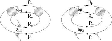
Figure 1: The diagrams with four Green’s functions in the thermodynamic potential which produce the anomalous term in the spin susceptibility. $\mathbf{p}_{+}$ and $\mathbf{p}_{-}$ indicate the directions of the momenta of electrons: $\mathbf{p}_{+}\approx-\mathbf{p}_{-}$. The chemical potential shifts $\delta\mu_{1}$ and $\delta\mu_{2}$ has been introduced in each of the two pairs of Green’s function. The spin-susceptibility can be generated from these diagrams by taking the second derivative with respect to $\delta\mu_{1,2}$. The triangles attached to the external vertices indicate the Fermi-liquid renormalization of the static spin vertices.

Let us discuss the origin of the anomalous temperature dependences. The calculation of interaction corrections to a thermodynamic quantity requires a summation over bosonic frequency $i\omega_{n}$. Transforming the sum into an integral along the real frequency axis results in an integral of the form $\int{d}\omega\coth(\beta\omega/2)f(\omega)$. If $f(\omega)$ is smooth and regular in the vicinity of $\omega=0$, the standard Sommerfeld expansion will involve only even powers of temperature. In order to get a term with an odd power of temperature (e.g., linear in $T$ correction to the spin-susceptibility), $f$ should be non-analytic preventing the Taylor expansion at $\omega=0$. Let us see how such non-analyticity develops in the case of the 2D electron gas. It is shown in Appendices B and D that both a $2p_{F}$-pair of Green’s functions and a pair in the Cooper channel have non-analytic parts (edge parts). Together these edge parts act as a sort of an ”edge-mode” propagating in the opposite directions. In the case of a $2p_{F}$-pair they are denoted as $\Pi_{r}$ and $\Pi_{l}$, i.e., ”right” and ”left”, reflecting the combinations $\omega\pm{v}_{F}\delta{q}$ in the denominators of Eq. (15). In the case of a pair in the Cooper channel the left and right edges of the branch-cuts in $\Psi$ play a similar role, see Eqs. (53) and (61). A diagram in the thermodynamic potential with the two edges running on each other produces the anomalous temperature dependence in the spin susceptibility because of its high sensitivity to the temperature and magnetic field at the point when they touch, see Fig. 2. The spectral weight of the edge-modes is much weaker compared to that of the usual quasiparticles, e.g., phonons. However, taking derivative with respect to an external parameter, a magnetic field in the case of the spin susceptibility, makes the spectral weight singular. As a result, the edge modes become active and are able to generate a non-analytic $f$ at $\omega=0$.

To get a clue of the origin of the discussed non-analytic terms, the following analogy may be useful. As it has been mentioned, a product of two propagators of the edge modes running on each other generates non-analytic terms in the spin susceptibility. With this in mind, consider an ensemble of one-dimensional right- and left-moving particles turning into each other due to a mixing matrix element. In such an auxiliary system, the diagrammatic expansion with respect to the mixing amplitude would suffer from strong ”infrared” divergences due to the degeneracy of the right- and left-moving particles at $q=0$. In particular, in the second order in mixing the thermodynamic potential has a term $\sim V_{mix}^{2}T\sum\int{d}q(\omega_{n}^{2}+q^{2})^{-1}$. The avoiding of the level crossing leads to the restructuring of the ground state of this system with the gap opening at $q=0$. Coming back to the non-analytic term in spin susceptibility in 2D at a finite temperature, we can see that the magnetic field $H$ (multiplied by the interaction amplitude) acts as the mixing matrix element in the subsystem of the edge modes. The considered diagrams are not divergent, because the spectral weight of the edge-modes is much weaker compared to the usual quasiparticles, e.g., phonons. Therefore, there are no enough resources for restructuring of the ground state. In addition, being composite objects, the edge modes are smeared by the temperature through the Fermi-Dirac function $n_{F}$ of the two fermions from which they are made of. Nevertheless, they still are able to produce the anomalous terms in the thermodynamic potential which appear as a trace of the mentioned above divergences in the expansion with respect to mixing amplitude in the auxiliary system. The analogy with auxiliary system also helps to understand the dependence on the order of taking the limits $H\rightarrow 0,T\rightarrow 0$. This dependence is similar to the competition between the value of the mixing matrix element and the energy of the particles in the auxiliary system, provided that the energy is substituted by the temperature in the original system of interacting electrons.

In Apppendices we show how the non-analytic (edge) parts in the product of two pairs of Green’s functions generate anomalous dependencies in the thermodynamic potential. With this experience let us now discuss possible generalizations of this mechanism. In diagrams defining the spin susceptibility there are two differentiations with respect to the magnetic field. The calculation of the term with two pairs indicates that for nucleating the non-analyticity in the thermodynamic potential the quasiparticles involved in the differentiation have to be constrained by the conservation of momentum and energy. For the product of two pairs these constraints are imposed automatically. Since for the more complicated diagrams this may not be the case, in identifying other non-analytic terms it is important to preserve this feature. Consequently, in the thermodynamic potential only those diagrams are essential that can be arranged as a closed ladder loop, and where only the Green’s function within the sections of the ladder are differentiated with respect to the magnetic field (by section we understand a pair of Green’s function describing a propagation of a pair of quasiparticles between the scattering events).

Organizing a diagram in the form of a ladder can be performed as follows. (In the discussion below the closed ladder loop should be not confused with the fermionic loops). If the Green functions marked by the differentiation belong to two different fermionic loops and there exists at least one another pair such that removing this group of Green’s functions (articulation quadruplet in the terminology of Ref. Dominicis1964, ) will split the diagram into two disconnected pieces, then these Green’s functions nucleate the ladder. Obviously, the Green’s functions that split the diagram are constrained by the conservation of energy and momentum. When such splitting requires more than one supporting pair, the non-analytic parts, which are a goal of our studies, are smeared by the additional integrations and this diagram cannot generate the linear in temperature term in spin susceptibility. When the two differentiated Green’s functions belong to the same fermionic loop, one first chooses another fermionic loop and repeats the procedure. Namely, it is needed to find another supporting pair of Green’s functions within the second loop which allows splitting the diagram into disconnected pieces. This completes the procedure of arranging the differentiated Green’s functions as a part of a ladder.

Unlike the one-dimensional case, the renormalizations in the Cooper and $2p_{F}$ channels are not mutually cross-coupled by the logarithmic corrections in two dimensions. This makes the Cooper channel the only one in which terms logarithmically divergent in temperature are generated. Besides that, in the treatment of the Cooper ladder we can consider its crossbars while ignoring their non-analytic parts originating from the $2p_{F}$ channel. We rely here on that (i) the non-analytic parts in the $2p_{F}$-scattering are small unless they are differentiated (notice that all the differentiated Green’s functions have been attributed to the Cooper ladder here), and more importantly that (ii) the non-analyticity generated in another channel is smeared out. That’s why for the calculation of the anomalous terms generated in the Cooper channel it is enough to consider a ladder assuming that the crossbars in the Cooper ladder are analytic.twodiff On these grounds, for the analysis of the non-analytic temperature dependences we can use as a starting point the conventional theory of the Fermi-liquid systems.

III Physical consequences of the renormalizations in the Cooper channel.

Cooper’s logarithms lead to renormalizations of the linear in $T$ term in the spin-susceptibility generated in the Cooper and $2p_{F}$ channels (see Appendix C for details):

$$\delta\chi=\nu\frac{T}{\epsilon_{F}}|\Gamma^{C}(\pi)_{T}|^{2}\,,$$ (1)

where $\nu=m/2\pi$ is the density of states per one species ($m$ is the effective mass which includes Fermi liquid renormalizations), and we omit the factors $(g\mu_{B}/2)$ everywhere. The renormalized backward scattering amplitude $\Gamma^{C}(\pi)$ is

$$\Gamma^{C}(\pi)_{T}=\sum_{n}(-1)^{n}\gamma_{n}(T),\qquad{\gamma}_{n}({T})=\frac{\Gamma_{n}^{C}}{1+\Gamma_{n}^{C}\ln\Lambda/{T}}\,.$$ (2)

Here $\gamma_{n}(T)$ are the renormalized Fourier harmonics amplitudes in the Cooper channel; $\Gamma_{n}^{C}$ are bare amplitudes defined at a large energy scale $\sim\epsilon_{F}$. This result is in full correspondence with the renormalization group equation for the angle-dependent amplitude $\Gamma^{C}(\theta)$ in the Cooper-channel. The fact that the amplitudes $\gamma_{n}(T)$ undergo strong renormalizations with temperature leads to important physical consequences which we now discuss.

When the temperature is reduced, the amplitudes $\gamma_{n}(T)$ which have a positive value are renormalized to zero, while those that initially are negative grow in magnitude. The initial (bare) value of $\Gamma^{C}(\pi)$ is most probably dominated by the zero-harmonic amplitude. It is naturally to expect that this harmonic is repulsive, and therefore when the temperature is lowered it dies out. In the intermediate region of temperatures when negative amplitudes are still small, i.e., when $1/|\Gamma_{n}^{C}|>\ln\Lambda/T>1/\Gamma_{0}^{C}$, the temperature dependence of the spin susceptibility is

$$\delta\chi\approx(\nu/\epsilon_{F})\;\frac{T}{(\ln\Lambda/T)^{2}}\,.$$ (3)

This result has been also obtained in Ref. [georg, ] using a technique developed recently for the ballistic systems.Efetov2006

As the temperature is lowered, the negative amplitudes start to grow. There are general reasons why the negative amplitudes are always present for some harmonics.Kohn1965 The largest negative amplitude, $\gamma_{n}=\gamma^{C}$, is most important as this amplitude grows most rapidly approaching the Cooper instability. When the amplitude $|\gamma^{C}(T)|$ becomes of order of unity, it acquires an essential temperature dependence. At small enough temperatures, when the renormalized to zero positive harmonics are suppressed, see Eq. (3), the temperature dependence of the growing negative amplitude $\gamma^{C}(T)=\Gamma^{C}/(1+\Gamma^{C}\ln\Lambda/{T)}$ prevails and can determine the temperature behavior of the spin susceptibility. This may cause a non-monotonic behavior in $\delta\chi(T)$. For the purpose of illustration, we will discuss the temperature dependence in the spin susceptibility leaving only the most rapidly growing amplitude $\gamma^{C}(T)$. In this case the temperature dependence of $\delta\chi(T)\varpropto T\gamma^{C}(T)^{2}$ is determined by two competing terms:

$$d\delta\chi/dT = (\nu/\epsilon_{F})[\gamma^{C}(T)^{2}+2T\gamma^{C}(T)(d\gamma^{C}(T)/dT)]$$ (4)

$$= (\nu/\epsilon_{F})(\gamma^{C}(T)^{2}-2|\gamma^{C}(T)|^{3}).$$

This expression changes its sign when $-\gamma^{C}(T)>1/2$.

Let us now consider the present experimental situation. Prus2003 The data indicate a noticeable temperature dependence of the spin susceptibility at $T\gtrsim 2K$, which is too strong to be attributed to the conventional Fermi-liquid corrections as a possible explanation. On the other hand, the possibility that this temperature increase is due to the presence of a large portion of free localized magnetic moments is probably not very realistic; at metallic densities that are $3\div 4$ times higher than the critical density $n_{c}$, the localized moments should be coupled by the RKKY interaction. Here we look at the observed temperature dependence from the point of view of the non-analytic corrections discussed in the paper.

The observed trend of the temperature dependence corresponds to decrease of the spin susceptibility with temperature. Equation (3) predicts, however, an opposite trend. The explanation of the experiment may be attributed to the non-monotonic behavior of the spin susceptibility due to temperature renormalizations of the negative amplitudes $\gamma_{n}$, as has been discussed above. In Ref. [Prus2003, ] the data are presented for $n/\chi(T)$, where $n$ is the density of the 2D electron gas. For silicon MOSFET (there are two valleys) the density $n=p_{F}^{2}/\pi$. For the degenerate Fermi gas with two valleys the unrenormalized spin susceptibility $\chi_{0}=4\nu$ and the ratio $n/\chi_{0}=p_{F}^{2}/2m$. In the presence of two valleys the expression for $\delta\chi$ as given by Eq. (1) should be multiplied by the factor $4$, i.e., $\delta\chi=4\nu(T/\epsilon_{F})\gamma^{C}(T)^{2}$. Since the temperature corrections are relatively small, one can expand $n/\chi$:

$$\delta(n/\chi)\approx\frac{n}{\chi_{0}^{2}}(-\delta\chi)=-T\gamma^{C}(T)^{2}\,.$$ (5)

The main feature of this relation is that the temperature dependence of $\delta(n/\chi)$ is determined by the amplitude $\gamma^{C}(T)$ only. Notice that the modification of the spin susceptibility by the Stoner factor drops out from $\delta(n/\chi)$ because of the renormalization of the two external vertices in $\delta\chi$, which are indicated by triangles in Fig. 1, see Eq. (27).

The dataPrus2003 exhibit a noticeable increase of $\delta(n/\chi)$ starting from $T\gtrsim 2K$ and correspond to $|\gamma^{C}(T)|\sim 1$ in Eq. (4). Such a value of the amplitude $\gamma^{C}(T)$ in the Cooper channel implies that the experiment has been performed at temperatures comparable with the temperature of the superconducting instability. Note, however, that in the disordered system studied in Ref. [Prus2003, ] the superconducting instability cannot fully develop for a non-zero harmonic ${\gamma}_{n}({T})=1/[(1/\Gamma_{n}^{C})^{-1}+\ln(\Lambda/\max{T,\tau}_{elastic}^{-1}){]}$, because the instability is blocked by disorder when ${\tau}_{elastic}^{-1}\gtrsim T_{c}$; here $T_{c}$ is the temperature of the Cooper instability in the dominant harmonic.

The experimental curves well in the metallic region correspond to $\epsilon_{F}\sim 30\div 40K$. We evaluate the bare value of the amplitude $\gamma^{C}$ as $\Gamma^{C}\sim-0.25\div-0.3$. Then, $\gamma^{C}(T)$ reaches the value $\gamma^{C}(T)=0.5,$ where $\delta\chi$ changes its sign, at temperatures $\sim 10K$. Would it not be blocked by disorder, the superconducting instability may occur at $T_{c}\sim 1K.$ The measurements are performed up to $T\lesssim 4K$. In the suggested explanation, the initial decrease with temperature of the spin susceptibility should be succeeded by an increase at larger temperatures, $T\gtrsim 10K$. The temperature range of the existing measurement is too small, however, to make this conclusions definite.

Two comments may be in place here. (i) The analysis of $\delta\chi(T)$ basing on Eq. (4) is only qualitative when $|\gamma^{C}(T)|\sim 1$. In fact, the situation is more complicated. The derivative $\partial\chi/\partial T$ is a series in $\gamma_{l}(T)$ which does not reduce to Eq. (4):

$$d\delta\chi/d{T}=(\nu/\epsilon_{F})\sum\Big{[}(-1)^{l^{\prime}+l^{\prime\prime}}\gamma_{l^{\prime}}({T})\gamma_{l^{\prime\prime}}({T})$$

$$+c_{3}^{l^{\prime}l^{\prime\prime}l^{\prime\prime\prime}}\gamma_{l^{\prime}}({T})\gamma_{l^{\prime\prime}}({T})\gamma_{l^{\prime\prime\prime}}({T})+\cdots\Big{]}\,.$$ (6)

The details are in the end of Appendix C. To get a final conclusion concerning a non-monotonic behavior, one has to calculate for $|\gamma^{C}(T)|\sim 1$ the whole series in Eq. (6), which is hardly possible. (ii) Initial values of the non-zero harmonics in the Cooper channel are highly non universal. In addition, the destructive influence of the disorder can stop the renormalization of the amplitude of the dominant harmonic before it becomes noticeable. Taken together, these facts mean that the experimental situation may strongly vary from sample to sample.

In a separate publication PNAS2006 , we present an alternative explanation of the experimental situation. We consider repulsive scattering amplitudes only, $\Gamma_{n}^{C}>0$, that is, perhaps, more appropriate for a system studied in Ref. [Prus2003, ]. Since the repulsive scattering amplitudes scale to zero, a more delicate analysis is necessary there. One has to account for all three channels, i.e. to include the rescattering of particle-hole pairs in the zero-sound channel in addition to the Cooper and $2p_{F}$-scattering channels. In this way it is possible to explain the observed temperature dependence of the spin susceptibility, both in sign and temperature. (Note that the non-monotonic behavior may also occur here. The temperature dependence changes its sign when the logarithmic suppression of the repulsive amplitudes become ineffective, i.e., when $1/\ln(\epsilon_{F}/T)\gtrsim\gamma^{C}$.)

IV Concluding remarks.

A decade ago, the authors of Ref. [Belitz1996b, ] made an important conjecture, based on the power counting, that thermodynamic quantities in the 2D electron gas contain linear in $T$ dependences. They argued that similarly to one dimension, where the spin susceptibility depends logarithmically on the temperature,Larkin1973a the anomalous temperature terms should also exist in higher dimensions, albeit in a weaker form.

We believe that presented calculation of the spin susceptibility in 2D does not support this line of reasoning. Indeed, the temperature dependence of the spin susceptibility in one dimension (1D) originates from the logarithmic in temperature dependence of the Stoner enhancement calculated in the parquet renormalization scheme.Larkin1973a ; Affleck1994 In contrast to the Fermi liquid description (which is analyzed in terms of a propagation of two quasi-particles) and the parquet approximation (which is analyzed with the Sudakov cross-section of two Green’s functions), the anomalous terms in the thermodynamic potential in 2D develops only when two (or more) edge parts of the two-particle correlation functions act in the combined way. In particular, in 2D, unlike 1D, the temperature dependence of the spin susceptibility does not reduce to a mere renormalization of the Stoner factor. In our opinion, the physics of the temperature corrections in 2D is rather unique and is not a mere continuation of 1D logarithms.

It has been shown in Appendices A and D that both a $2p_{F}$-pair and a two-particle section in the Cooper channel have non-analytic parts (edge parts). In two dimensions the square root singularities of these edge parts are relatively weak. However, taking derivatives with respect to an external parameter, a magnetic field in our case, makes them more singular, i.e., activates them. Because of high sensitivity to the temperature and magnetic field, diagrams containing edge parts running on each other produce the anomalous terms in the spin susceptibility. When a diagram for the thermodynamic potential consists only of two pairs of quasiparticles, their edge parts are effective because the quasiparticles are constrained by the conservation of the momentum and energy. In this case the edge parts of the two pairs act together in a combined way. For more complicated diagrams the non-analytic pieces may be not constrained. Then they are smeared out by independent integrations and become ineffective. This leads us to the conclusion that for the anomalous temperature dependences the essential diagrams in the thermodynamic potential are ladder diagrams only. For the spin susceptibility the set of essential diagrams in the $2p_{F}$ and Cooper channels is organized in a way that the anomalous terms can be considered within the Cooper channel only. (This rearranging is necessary to avoid the double-counting of the two-section terms which, as has been found here, completely overlap in the $2p_{F}$ and Cooper channels.) We show next that one has to keep arbitrary number of sections in the Cooper channel ladder to collect all non-analytic terms in the spin susceptibility, i.e., not only a product of the two pairs. (This is because the singular part of a two-particle section in the Cooper channel depends on the ratio $\omega/qv_{F}$.) The truncation of the series in powers of the renormalized amplitudes is possible only when these amplitudes are small.

In Refs. [Galitski2005, ; GlazmanB2005, ] the possibility of strong renormalizations in the Cooper channel was neglected and the amplitude $\Gamma(\pi)$ was analyzed from the point of view of the Fermi-liquid renormalizations. These renormalizations are not related to the infrared logarithms, but they may be large near Pomeranchuk’s instability in one of the channels, e.g., near the Stoner instability in the case of the magnetism.Galitski2005 Since the amplitude $\Gamma(\pi)$ involves all angular harmonics, an instability in any of them can be important. In this paper we assumed that the discussed Fermi liquid system is not in the immediate proximity of any instability. In this respect our analysis emphasizing only the infrared renormalizations in the Cooper channel may be incomplete.

Finally, let us point out that when the Fourier harmonics amplitudes in the Cooper channel, $\Gamma_{n}^{C}$, are repulsive and scale to zero at low temperatures, the contributions to the spin susceptibility from the Cooper channel become unimportant. This situation is analyzed in a separate publication PNAS2006 , which is complementary to the present one. For vanishing Cooper amplitudes, the anomalous temperature terms are dominated by the non analytic contributions from the particle-hole pairs with small momentum transfer (zero-sound channel). Extending our analysis to particle-hole rescattering, we show that, exactly like in the Cooper channel, the two-section term in the zero-sound channel is dominated by the backward scattering. To avoid the double counting which now involves all three channels, the two-section term has been fully attributed to the Cooper channel, where it gets killed off by the logarithmic renormalizations of the repulsive amplitudes. We thus conclude that for the repulsive interaction the anomalous temperature corrections are determined by the ladder diagrams in the zero-sound channel with three and more rescattering sections.threesections

Appendix A Analytic properties of the product of two Green’s function with $q\approx 2p_{F}$

Consider a product of two Green’s functions summed over the momentum and the energy as a function of the transferred energy $i\omega_{n}$ and momentum $\mathbf{q}$

$$[GG]_{i\omega_{n},\mathbf{q}}=\int\frac{d^{2}p}{(2\pi)^{2}}\frac{n_{F}(\epsilon_{\mathbf{p}+\mathbf{q}}-\mu)-n_{F}(\epsilon_{\mathbf{p}}-\mu)}{\epsilon_{\mathbf{p}+\mathbf{q}}-\epsilon_{\mathbf{p}}-i\omega_{n}}\,,$$ (7)

where $n_{F}$ is the Fermi-Dirac distribution function $n_{F}(\epsilon)=[\exp(\beta\epsilon)+1]^{-1}$. We are interested in the analytic structure of Eq. (7) in the complex-$\omega$ plane when $q\equiv|\mathbf{q}|\approx 2p_{F}$. To get an idea about the analytic properties of a $2p_{F}$-pair of Green’s functions, let us start from the case when $\epsilon_{\mathrm{p}}=(p_{\parallel}^{2}+p_{\perp}^{2})/2m$. We first shift the momentum $\mathbf{p}+\mathbf{q}$ to $\mathbf{p}$ in the first term in the numerator and write the $d^{2}p$-integration as $d^{2}p=dp_{\parallel}dp_{\perp}$, where $p_{\parallel}$ is along the direction of $\mathbf{q}$. Then, the variable $p_{\perp}$ drops from the denominator and enters only via $n_{F}(\epsilon_{p}-\mu)$. This parametrization allows us to introduce the ”spectral density” $\rho(p_{\parallel})$ which determines the dependence on the chemical potential and the temperature

$$\rho(p_{\parallel})=\int_{-\infty}^{+\infty}\frac{dp_{\perp}}{2}n_{F}(\epsilon_{\mathbf{p}}-\mu)\,.$$ (8)

After that get an expression for the $2p_{F}$-pair in the form of the Lehmann-like representation in the complex-$\omega$ plane

$$[GG]_{\omega,\mathbf{q}}=\frac{m^{1/2}}{4\pi v_{F}}\left(\Pi_{l}(q,\omega)-\Pi_{r}(q,\omega)\right)\,,$$ (9)

where the functions $\Pi_{l}(q,\omega)$ and $\Pi_{r}(q,\omega)$ are defined as

$$\frac{m^{1/2}}{4\pi v_{F}}\Pi_{l,r}(q,\omega)=\frac{m}{2\pi q}\int\frac{dp_{\parallel}}{\pi}\frac{\rho(p_{\parallel})}{p_{\parallel}-(m/q)(\omega\pm q^{2}/2m)}\,.$$ (10)

Here $\pm$ in the denominator corresponds to $\Pi_{l}$ and $\Pi_{r}$, respectively. From now on, in this Appendix we consider the temperature to be zero. [The non-zero temperature can be restored with the help of equation (18) as it is explained below.] At $T=0$ the integral in Eq. (8) is easily evaluated: $\rho(p_{\parallel})_{T=0}=\sqrt{p_{F}^{2}-p_{\parallel}^{2}}\theta(p_{F}-p_{\parallel})$. In the complex-$\omega$, plane $\Pi_{l,r}(\omega)$ considered as a function of the variable $u_{\pm}=(m/qp_{F})(\omega\pm{q}^{2}/2m)$, have the following analytic form

$$\frac{m^{1/2}}{4\pi v_{F}}\Pi_{l,r}=\frac{mp_{F}}{2\pi q}F(u_{\pm});$$

$$\qquad F(u)=\int_{-1}^{1}\frac{dx}{\pi}\frac{\sqrt{1-x^{2}}}{x-u}=-u+\sqrt{u-1}\sqrt{u+1}\,.$$ (11)

Here the square roots should be understood as having a branch cut directed to the right on the real axis. Correspondingly, $F(u)$ has a branch cut between $-1$ and $1$ in the complex-$u$ plane. On the upper side of the branch cut the imaginary part of $F(u)$ is positive; the real part originating in the square root term is positive to the right of the branch cut and is negative to the left of it.

Figure 2: Illustration of the analytic structure of the $2p_{F}$ pair of Green’s functions. The horizontal axis is $\mathrm{Re}\,\omega$ and the vertical axis is $q$. The parabolas show the position of the edges of the branch cuts of $\Pi_{l,r}$ in the $q,\mathrm{Re}\omega$-plane. The dashed lines show the branch cuts of $\Pi_{r,l}$ for two typical values of $q$: the $\Pi_{r}$-part has branch cuts between the two right-looking parabolas, and $\Pi_{l}$ has branch cuts between the two left-looking parabolas. The rectangle marks the region where the edges of the two branch cuts of two $2p_{F}$ pairs are close to each other. The meeting of two edges leads to non-analytic behavior of the thermodynamic potential.

Only the second term in $F(u)$ containing the square roots can be responsible for non-analytic behavior in the thermodynamic potential. The non-analytic temperature dependence in the product of four Green’s functions originates from region marked by dashed-line rectangle in Fig. 2 where the edges of the branch cuts of $\Pi_{r}$ and $\Pi_{l}$ are close to each other. This makes the contribution from this region very sensitive to the magnetic field and temperature smearing.

For the calculation of the non-analytic term in the spin susceptibility it is enough to use an appropriate approximation for $2p_{F}$-pair in the region marked by a dashed-line rectangle in the Fig. 2. This involves the $u=-1$ edge of branch cut in $\Pi_{r}$ and the $u=1$ edge of the branch cut in $\Pi_{l}$. In the following we omit the smooth terms in $F(u)$. It can be checked by an explicit calculation that the first term in $F(u)$ does not to contribute to the anomalous temperature behavior.

The spectrum of electrons is not considered to be quadratic, like in Eqs. (10) and (11), but we still assume the spherical symmetry. The generalization for a non-spherical spectrum can be done, if needed. To devise an adequate approximation for $\Pi_{lr}$, we consider again the product of two Green’s functions, $\big{[}G_{+}G_{-}\big{]}_{\delta q,i\omega}$ describing the propagation of two quasiparticles with the momenta $\mathbf{p}_{+}$ and $\mathbf{p}_{-}$, which are almost opposite to each other. The transferred momentum $\mathbf{q}=\mathbf{p}_{+}-\mathbf{p}_{-}$ is close to $2p_{F}$, and $\delta q=|\mathbf{q}|-2p_{F}$ describes a small deviation from $2p_{F}$. We choose the following parametrization where $\mathbf{p}_{F}$ is a vector directed along $\mathbf{q}$:

$$\mathbf{q}\;\;= \;\;2\mathbf{p}_{F}+\delta\mathbf{q},$$

$$\mathbf{p_{-}}= -\mathbf{p}_{F}+\delta\mathbf{p}\,.$$ (12)

To reproduce the correct threshold behavior we keep minimal terms in the expansion in $p_{\parallel}$ and $p_{\perp}$. We linearize the energy spectrum around the points $\pm\mathbf{p}_{F}$ in the direction perpendicular to the Fermi surface, but preserve the quadratic momentum dependence in the direction parallel to the Fermi surface to account for the Fermi surface curvature

$$\epsilon_{\mathbf{p}_{-}}-\mu_{0}= -v_{F}\delta p_{\parallel}+p_{\perp}^{2}/2m$$

$$\epsilon_{\mathbf{p}_{+}}-\mu_{0}= \;\;v_{F}(\delta p_{\parallel}+\delta q)+p_{\perp}^{2}/2m\,.$$ (13)

We obtain the following approximation for $\Pi_{r,l}(\omega)$ at zero temperature

$$\frac{m^{1/2}}{4\pi{v}_{F}}\Pi_{l,r}(q,\omega)$$

$$\;\;=\frac{1}{2\pi}\int\frac{dp_{\parallel}dp_{\perp}}{2\pi}\;\frac{n_{F}\Big{(}\pm{v}_{F}(\delta p_{\parallel}+\delta q)+p_{\perp}^{2}/2m-\delta\mu\Big{)}}{v_{F}(2\delta p_{\parallel}+\delta q)-\omega}\,,$$ (14)

where $\pm$ corresponds to $\Pi_{l}$ and to $\Pi_{r}$, respectively.

Having in mind the calculation of the spin susceptibility from the correction to the thermodynamic potential we introduce a shift of the chemical potential $\mu=\mu_{0}+\delta\mu$ in Eq. (14). Introducing $x=2v_{F}(\delta p_{\parallel}+\delta{q})\pm 2\delta\mu$ in $\Pi_{r}$ and $\Pi_{l}$, respectively, we obtain after integrating over $p_{\perp}$ the following expressions for $\Pi_{l,r}$

$$\Pi_{l}(\delta{q},\omega)_{T=0}=\int\frac{dx}{\pi}\frac{\sqrt{-x}\theta(-x)}{x-(\omega+v_{F}\delta q-2\delta\mu)}$$

$$\Pi_{r}(\delta{q},\omega)_{T=0}=\int\frac{dx}{\pi}\frac{\sqrt{x}\theta(x)}{x-(\omega-v_{F}\delta q+2\delta\mu)}\,.$$ (15)

These expressions correspond to Eq. (10) within the region marked by dashed-line rectangle in Fig. 2. Here the functions $\Pi_{l,r}$ are defined with positive square roots in the numerator. In this Lehmann-like representation, $\Pi_{l}$ describes the square root function with the branch cut directed to the left on the real axes of $\omega$-plane, while $\Pi_{r}$ describes the function with the branch cut directed to the right. [Indices $l$ and $r$ correspond also to the direction of ”propagation” in the combinations $\omega\pm{v}_{F}q$.] Both $\Pi_{l}$ and $\Pi_{r}$ have a positive imaginary part on the upper side of their branch cuts in the complex $\omega$-plane.

Let us conclude this Appendix by a comment on Eq. (15). This equation gives a representation of the edge parts of $2p_{F}$-pair of Green’s functions as two pieces, $\Pi_{r}$ and $\Pi_{l}$, in the region inside the dashed-line rectangle in Fig. 2. Together these edge parts act as a sort of an ”edge-mode”; we mean the combination $\omega\pm{v}_{F}(q-2p_{F})$ in the denominators of Eq. (15). The square root spectral weight of these edge-modes is much weaker compared to the usual quasiparticles, e.g., phonons. However, taking derivative with respect to an external parameter, a magnetic field in our case, makes the spectral weight singular. As a result, these edge modes become active. In Appendices B and C we show that, because of the unusual sensitivity to the temperature and magnetic field, a diagram in the thermodynamic potential with two propagators of the edge modes running on each other produces the anomalous temperature dependence in the spin susceptibility of the interacting electron gas.

Appendix B Anomalous terms generated by two $2p_{F}$-pairs.

The term in the thermodynamic potential with four Green’s functions which produces the anomalous term in the spin susceptibility is

$$\delta\Omega_{2}(T,h)=-(1/2)g_{4}^{\uparrow\downarrow}(T;h,-h)|\Gamma(\pi)|^{2}\,,$$ (16)

where $g_{4}(\delta\mu_{1},\delta\mu_{2};T)$ signifies the product of the two pairs of Green’s functions with the chemical potential shifted in two pairs by $\delta\mu_{1}$ and $\delta\mu_{2}$, correspondingly; arrows indicate spin and we consider a Zeeman energy $h=(g\mu_{B}/2)H$ as the source of a shift of the chemical potentials. The factor $1/2$ can be obtained from the comparison with the second order term in the perturbation theory for the thermodynamic potential. [There are two such contributions, with $\uparrow\downarrow$ and $\downarrow\uparrow$ arrangements of spins in the two pairs of Green’s functions, which has been accounted for by the factor $1/2$ in Eq. (16)]. The terms with the parallel spin projections in the two pairs of Green’s functions, i.e., $g_{4}^{\uparrow\uparrow}(T;h,h)$ and $g_{4}^{\downarrow\downarrow}(T;h,h)$, do not contribute to the anomalous term.

Having in mind the correction to the thermodynamic potential $\delta\Omega_{2}$ given by Eq. (16), we now perform the sum over Matsubara frequency $i\omega_{n}$. The standard manipulation leads to

$$g_{4}(T;\delta\mu_{1},\delta\mu_{2})=\frac{mp_{F}}{(4\pi v_{F})^{2}}\int\frac{d\delta q}{\pi}\int\frac{d\omega}{2\pi}\coth\frac{\beta\omega}{2}\,$$

$$\Big{\{}\mathrm{Im}\,\big{[}\Pi_{l}(\delta\mu_{1})-\Pi_{r}(\delta\mu_{1})\big{]}_{T}\;\mathrm{Re}\,\big{[}\Pi_{l}(\delta\mu_{2})-\Pi_{r}(\delta\mu_{2})\big{]}_{T}$$

$$\;+(\delta\mu_{1}\leftrightarrow\delta\mu_{2})\Big{\}}\,.$$ (17)

The signs of different terms in this expression are completely determined by the analytical properties of functions $\Pi_{r,l}$. Only the cross-product terms, i.e., $\Pi_{l}\Pi_{r}$, behave sharply in the vicinity of $\omega=0$, and therefore are responsible for non-analytic terms in the thermodynamic potential. It can be checked directly that in a product of, let us say, $\Pi_{r}$ with a regular function its square root singularity disappears after the $q$-integration. For similar reasons, the products $\Pi_{l}\Pi_{l}$ and $\Pi_{r}\Pi_{r}$ yield regular functions in frequency. On the contrary, in the product $\Pi_{l}\Pi_{r}$ the edges of the two branch cuts run on each other, preventing the smearing of the singularity.

The temperature dependence in the functions $\Pi_{l,r}$ can be restored with the help of the relation

$$\Pi(\omega)_{T}=\int ds\left(-\frac{\partial n_{F}(s)}{\partial s}\right)\Pi(\omega-s)_{T=0}$$ (18)

which follows from the identity

$$n_{F}(\omega)_{T}=\int ds\left(-\frac{\partial n_{F}(s)}{\partial s}\right)n_{F}(\omega-s)_{T=0}\,.$$ (19)

Performing the $q$-integration in Eq. (17) one gets

$$g_{4}(\delta\mu_{1},\delta\mu_{2})_{T}=-\frac{\nu^{3}}{8\epsilon_{F}}\int d\omega ds_{1}ds_{2}\frac{\partial n_{F}(s_{1})}{\partial s_{1}}\frac{\partial n_{F}(s_{2})}{\partial s_{2}}\,\times$$

$$\quad\coth\frac{\beta\omega}{2}\Big{[}(\omega+\delta\mu_{1}-\delta\mu_{2}+s_{1}-s_{2})^{2}\mathrm{sign}(\omega+\Delta+s_{1}-s_{2})\Big{]}\,,$$ (20)

The obtained expression depends on the relative shift $\Delta=\delta\mu_{1}-\delta\mu_{2}$ of the chemical potential in the two pairs of Green’s functions. The signum function in this expression appears because the contributions with $\mathrm{Im}\,\Pi_{r}(\delta\mu_{1})\;\mathrm{Re}\,\Pi_{l}(\delta\mu_{2})$ and $\mathrm{Re}\,\Pi_{r}(\delta\mu_{1})\;\mathrm{Im}\,\Pi_{l}(\delta\mu_{2})$ have opposite signs. The expression (20) contains the needed non-analytic frequency dependence through the factor $\mathrm{sign}(\omega+\delta\mu_{1}-\delta\mu_{2})$. This factor compensates the odd-in-frequency behavior of $\coth$ allowing for the cubic $\Delta^{2}T$ term in the expansion of $g_{4}(\Delta,T)$ which produces the linear in $T$ term in the spin susceptibility. Notice that the expression obtained in Eq. (20) explains how the dependence on the order of taking the limits $H\rightarrow 0,T\rightarrow 0$ appears in the thermodynamic potential. At $T\ll H$ the temperature dependent terms in the thermodynamic potential vanishes as $T^{3}$. To calculate the spin susceptibility one has to take the opposite limit, $H\ll T$.

Let us first consider a contribution to the transverse spin susceptibility, as illustrated in Fig. 1. Notice that there are no ”drag” diagrams for the transverse spin susceptibility, because Green’s functions attached to the external vertices $\sigma^{\pm}$, carry opposite spins. The spin susceptibility correction which corresponds to these diagrams is

$$\delta\chi=\,2(\chi_{0}/\nu)\,\left(\frac{1}{2}\frac{\partial^{2}g_{4}(T;\delta\mu_{1},\delta\mu_{2})}{\partial\delta\mu_{1}^{2}}\Big{|}_{\begin{array}[]{c}{\scriptscriptstyle\delta\mu_{1}=0}\\ {\scriptscriptstyle\delta\mu_{2}=0}\end{array}}\right)\,|\Gamma(\pi)|^{2}\,.$$ (21)

Here the ratio $(\chi_{0}/\nu)$ accounts for the factors arising in the calculation of the spin susceptibility from the corresponding diagram with $\sigma^{+}$ and $\sigma^{-}$ at the vertices. Factor $2$ accounts for a spin trace in the upper bubble in the diagrams presented in Fig. 1. The derivative in the brackets generates an expression with six Green’s functions corresponding with the correct coefficient.

The $\omega$ integration in Eq. (21) can be cast in the form

$$\frac{1}{2}\frac{\partial^{2}g_{4}(T;\delta\mu_{1},\delta\mu_{2})}{\partial\delta\mu_{1}^{2}}\Big{|}_{\begin{array}[]{c}{\scriptscriptstyle\delta\mu_{1}=0}\\ {\scriptscriptstyle\delta\mu_{2}=0}\end{array}}=$$ (24)

$$\qquad-\frac{\nu^{3}}{8\epsilon_{F}}\int_{-\Lambda}^{\Lambda}d\omega-\int d\omega\frac{2-\beta\omega\coth\frac{\beta\omega}{2}}{\cosh\beta\omega-1}$$ (25)

The first term here is proportional to the ultraviolet cutoff. Since it does not depend on the temperature, it will be not considered here. [In fact, the traces of this term reveal themselves in the $\Gamma^{3}$ terms which cannot be reduced to the renormalization of the amplitude $\Gamma(\pi)$ by the rescattering in the Cooper channel.] Omitting the factor $(g\mu_{B}/2)^{2}$, we obtain for the anomalous contribution in the spin susceptibility

$$\delta\chi=\nu\,|\nu\Gamma(\pi)|^{2}\,\frac{T}{\epsilon_{F}}\,,$$ (26)

which coincides with the result of previous calculations, see Refs. [Galitski2005, ; GlazmanB2005, ].

Let us clarify the role of the amplitude $\Gamma(0)$ with the scattering angle $\theta-\theta^{\prime}\approx 0$ in the linear in $T$ term in the spin susceptibility. In the diagrams with two pairs of Green’s functions, which can also be looked at as two pairs with the momentum transfer close to $2p_{F},$ the scattering amplitude $\Gamma(0)$ can be mixed with $\Gamma(\pi)$ or used twice alone. With one exception, these are one-loop diagrams which cannot contribute to the spin susceptibility (all spin projections are the same and they don’t have part with a difference in the chemical potential). The only exception is the diagram with two loops. In each loop the two Green’s functions have close momenta, but their directions are opposite in two loops; the spin projections are also opposite in the two loops. When rearranged as two pairs with the momentum transfer close to $2p_{F}$, they have needed shifts of the chemical potentials, but still $\delta\mu_{1}=\delta\mu_{2}$, and therefore the corresponding $g_{4}(\delta\mu_{1},\delta\mu_{2})$ does not contribute to the spin susceptibility. With this comment we fixed the arrangement of the dashed lines in Fig. 1. We see that the magnetic field dependence drops out from $g_{4}$ unless there are two loops, each with a $2p_{F}$-pair of Green’s function, and with the spin projections directed oppositely in each of the loops.

The performed calculation of the anomalous term in the spin susceptibility demonstrates that it is generated by the pole parts of Green’s functions close the Fermi surface. It follows from this fact that the Fermi liquid renormalizations of the $\delta\chi$ originating from the two external vertices (triangles in the Fig. 1) are equal to the square of the Fermi liquid parameter $1/(1+G_{0})$ responsible for the renormalization of the Pauli spin susceptibility. Including these renormalizations the temperature correction takes the form

$$\delta\chi=\frac{\nu}{(1+G_{0})^{2}}|\nu\Gamma(\pi)|^{2}\,\frac{T}{\epsilon_{F}}\,.$$ (27)

The longitudinal spin susceptibility can also be obtained in the same way by taking the second derivative with respect to the magnetic field, $\chi=-\partial^{2}\Omega_{2}/\partial h^{2}$. Notice that in the case of the transverse spin susceptibility the coefficient $2(\chi_{0}/\nu)$ originates from two independent spin traces in Fig. 1. In the case of the longitudinal spin susceptibility there is no spin traces anymore, but the additional factor 4 in this case originates from the differentiation of $g_{4}(T;h,-h)$ in Eq. (16) with respect to $h$ rather than with respect to its first argument only as in Eq. (21). As a result one obtains the same expression as in Eq. (26).

Appendix C Non-analytic terms in the Cooper channel

In Appendix  B it has been assumed from the very beginning that the transferred momentum $q$ is close to $2p_{F}$. We start the present Appendix with an alternative treatment of the term $\delta\Omega_{2}$ which now will be recalculated as two sections in the Cooper channel. Here we will not assume a priory that only backward scattering is important. Remarkably, we obtain this fact as a result of independent calculation. Finally, we extend the consideration of the anomalous terms by analysis of the Cooper ladder in the thermodynamic potential.

C.1 Calculation of two pairs in the Cooper channel.

We start with a pair of Green’s functions in the Cooper channel

$$[G(\delta\mu_{1})G(\delta\mu_{2})]_{q,i\omega_{n}}$$

$$= \int\frac{d^{2}p}{(2\pi)^{2}}T\sum_{i\epsilon_{n}}G_{\mathbf{p}+\mathbf{q}/2}(i\epsilon_{n}+i\omega_{n};\delta\mu_{1})\;G_{-\mathbf{p}+\mathbf{q}/2}(-i\epsilon_{n};\delta\mu_{2})$$

$$= \frac{1}{2}\int\frac{d^{2}p}{(2\pi)^{2}}\frac{\tanh\frac{\beta}{2}\big{(}\xi_{\mathbf{p}+\mathbf{q}/2}-\delta\mu_{1}\big{)}+\tanh\frac{\beta}{2}\big{(}\xi_{-\mathbf{p}+\mathbf{q}/2}-\delta\mu_{2}\big{)}}{\xi_{\mathbf{p}+\mathbf{q}/2}+\xi_{-\mathbf{p}+\mathbf{q}/2}-\delta\mu_{1}-\delta\mu_{2}-i\omega_{n}}\,.$$ (28)

where $\xi_{\mathbf{p}}=\epsilon_{\mathbf{p}}-\mu$ and $q=|\mathbf{q}|$. To account for the effect of magnetic field, we introduced the shift of the chemical potential $\delta\mu=\pm{h}$ depending on the sign of spin projection. We now shift the energy variable $\xi_{\mathbf{p}}$ by $(\delta\mu_{1}+\delta\mu_{2})/2$. The obtained expression depends on the relative shift $\Delta=\delta\mu_{1}-\delta\mu_{2}$ of the chemical potential in the two Green’s functions. Only the pairs with the opposite spin projections retain the dependence on the magnetic field $h$; the anomalous temperature terms are not sensitive to the overall shift of the chemical potential. Finally, after making analytical continuation to the complex-$\omega$ plane $i\omega_{n}\rightarrow\omega$ we obtain:

$$[G(\delta\mu_{1})G(\delta\mu_{2})]_{q,\omega}$$

$$= \frac{1}{2}\int\frac{d^{2}p}{(2\pi)^{2}}\frac{\tanh\frac{\beta}{2}\Big{(}\xi+(qv_{F}/2)\cos\theta-\Delta/2\Big{)}}{2\xi-\omega}+$$

$$+\Delta\leftrightarrow-\Delta\,,$$ (29)

where $\theta$ is the angle between the momenta $\mathbf{p}$ and $\mathbf{q}$ in Green’s functions in Eq. (28); here we expand $\xi_{\mathbf{p}+\mathbf{q}/2}$ using the smallness of $q$ and introduce $\xi=\xi_{\mathbf{p}}$; i.e., $\xi_{\mathbf{p}+\mathbf{q}/2}=\xi+(qv_{F}/2)\cos\theta$. The result reproduces the Cooper logarithm multiplied by the single particle density of states (per spin). We use a variable $x=2\xi$ to obtain the expression in form of the Lehmann-like representation:

$$[GG]_{q,\theta,\omega}=\frac{\nu\pi}{4}\Big{(}\Psi(q,\theta,\omega+\Delta)_{T}+\Psi(q,\theta,\omega-\Delta)_{T}\Big{)}\,,$$ (30)

where

$$\Psi(q,\theta,\omega\pm\Delta)_{T}=\int\frac{dx}{\pi}\frac{\tanh\frac{\beta}{4}\big{(}x\pm\Delta-qv_{F}\cos\theta\big{)}}{x-\omega}\,.$$ (31)

The normalization of $\Psi(\theta)$ is such that the imaginary part of $\Psi$ approaches $\pm 1$ at large values of $\omega$. At zero temperature the hyperbolic tangent becomes the signum function. The temperature width of Fermi-Dirac function can be restored from $T=0$ function with the help of the relation

$$\Psi(\omega)_{T}=\frac{1}{2}\int ds\frac{\partial\tanh\frac{\beta s}{4}}{\partial{s}}\Psi(\omega-s)_{T=0}$$ (32)

that follows from the identity

$$\tanh\alpha{x}=\frac{1}{2}\int ds\frac{\partial\tanh\alpha{s}}{\partial{s}}\mathrm{sign}(x-s)\,.$$ (33)

The contribution to the thermodynamic potential from two sections (recall that by section we understand a pair of Green’s function describing a propagation of two quasiparticles between the scattering events) in the Cooper channel is given by

$$\Omega_{2}(\Delta)=-\frac{1}{2}\left(\frac{\pi}{2}\right)^{2}\int\frac{qdq}{2\pi}\frac{d\theta_{1}}{2\pi}\frac{d\theta_{2}}{2\pi}\;T\sum_{i\omega_{n}}$$

$$\;\Gamma^{C}(\theta_{1}-\theta_{2})\Upsilon(\theta_{2},q,i\omega_{n})_{T}\Gamma^{C}(\theta_{2}-\theta_{1})\Upsilon(\theta_{1},q,i\omega_{n})_{T}\,,$$ (34)

where $\Upsilon(\Delta)_{T}=\big{[}\Psi(\omega+\Delta)_{T}+\Psi(\omega-\Delta)_{T}\big{]}/2$, and $\Gamma^{C}(\theta)=\nu\Gamma(\theta)$ is dimensionless angle-dependent amplitude in the Cooper channel. Let us pass to the Fourier harmonics of the Cooper channel amplitudes, $\Gamma^{C}(\theta)=\sum_{n}e^{in\theta}\Gamma_{n}^{C}$. We assume that the amplitudes $\Gamma(\theta)$ are real and are even functions of $\theta_{1}-\theta_{2}$. This corresponds to real $\Gamma^{l}=\Gamma^{-l}$. The angular integration leads to the following expression for the contribution of two Cooper sections to the anomalous part of the thermodynamic potential

$$\Omega_{2}(\Delta)=-\frac{1}{2}\left(\frac{\pi}{2}\right)^{2}\int\frac{qdq}{2\pi}T\sum_{i\omega_{n}}$$

$$\;\Gamma_{l}^{C}\Upsilon_{l-m}(q,i\omega_{n})_{T}\Gamma_{m}^{C}\Upsilon_{m-l}(q,i\omega_{n})_{T}\,.$$ (35)

Here the angular harmonic $\Psi_{n}$ of function $\Psi(\theta)$ are defined as

$$\Psi_{n}=\int\frac{d\theta}{2\pi}e^{in\theta}\Psi(\theta)\,.$$ (36)

After transforming the frequency sum to the integral we obtain

$$\Omega_{2}(\Delta)=-\sum_{n,m}\frac{\Gamma_{n}^{C}\Gamma_{m}^{C}}{32}\int{qdq}\int{d\omega}\coth\frac{\beta\omega}{2}$$

$$\;\mathrm{Im}\,\big{\{}\Upsilon_{n-m}(q,\omega,\Delta)_{T}\Upsilon_{m-n}(q,\omega,\Delta)_{T}\big{\}}\,,$$ (37)

where the contour of $\omega$-integration is slightly shifted above the real axes.

Let us now turn to the calculation of the anomalous temperature term in the spin susceptibility. For the chemical potential shifts induced by the magnetic field $\Delta=2h$ and, therefore, $\delta\chi=-\frac{\partial^{2}}{\partial{h}^{2}}\Omega_{2}(2h)$. This yields

$$\delta\chi= \frac{1}{4\pi v_{F}^{2}}\int{d\omega}\coth\frac{\beta\omega}{2}\Gamma_{n}^{C}\Gamma_{m}^{C}\left\langle h_{nm}(\omega;s_{1},s_{2})\right\rangle_{T}$$

$$h_{nm}(\omega)= \frac{\pi}{2}\int{qdq}\mathrm{Im}\,\Big{\{}\Big{[}\frac{\partial^{2}}{\partial\omega^{2}}\Psi_{n-m}(q,\omega_{1})\Big{]}\Psi_{m-n}(q,\omega_{2})\Big{\}}$$

$$+(\omega_{1}\leftrightarrow\omega_{2})\,.$$ (38)

From now on, $q$ is an energy variable, i.e., $qv_{F}\rightarrow{q}$. This substitution leads to the factor $1/v_{F}^{2}=\pi\nu/\epsilon_{F}$ in the first line and makes $h_{nm}$ to be dimensionless. The notation $\langle\cdots\rangle_{T}$ means the integration over $s_{1,2}$ which originates from Eq. (32). In $h_{nm}$ the shifted frequencies $\omega_{1,2}=\omega-s_{1,2}$ have been introduced and here (and everywhere below) $\Psi(\omega)$ means $\Psi(\omega)_{T=0}$. Next, in Eq. (38) we replace the second derivative with respect to $\Delta$ by the second derivative with respect to $\omega$ and afterwards the limit $h\rightarrow 0$ has been taken. Notice that terms with the first derivatives vanish because $\partial\Upsilon(h\rightarrow 0)/\partial{h}=0$. The $q$-integrations in $h_{nm}$ yields (for details see Appendix D)

$$h_{nm}=-2\mathrm{sign}(\omega_{1}+\omega_{2})\,(-1)^{n-m}\,.$$ (39)

It is now necessary to perform the $\omega$ and $s_{1,2}$ integrations

$$\delta\chi=-\frac{\Gamma_{n}^{C}\Gamma_{m}^{C}(-1)^{n+m}}{2\pi{v}_{F}^{2}}\int\frac{ds_{1}ds_{2}}{4}{d\omega}$$

$$\coth\frac{\beta{\omega}}{2}\frac{d\tanh\frac{\beta{s}_{1}}{4}}{ds_{1}}\frac{d\tanh\frac{\beta{s}_{2}}{4}}{ds_{2}}\;\mathrm{sign}(2\omega-s_{1}-s_{2})\,.$$ (40)

The $\omega$-integration can easily be done with the use of the relation $\coth(\beta\omega/2)=2Td\ln\sinh(\beta\omega/2)/d\omega$. Transferring the frequency derivative from $\ln\sinh(\beta\omega/2)$ to $\mathrm{sign}(2\omega-s_{1}-s_{2})$ we get a $\delta$-function of frequency. The boundary term here corresponds to the first integral in the right hand side of Eq. (25). It does not depend on frequency and will be dropped. Passing to $u_{1,2}=\tanh{\beta{s}_{1,2}}$ as our new integration variables, we get an elementary integral. Finally,

$$\delta\chi=\nu\frac{T}{\epsilon_{F}}\sum\Gamma_{n}^{C}\Gamma_{m}^{C}(-1)^{n+m}\,.$$ (41)

The angular integration Eq. (34) covers all momentum directions in both Cooper sections. Nevertheless, the result given in Eq. (41) can be written in terms of the backward scattering amplitude only

$$\delta\chi=\nu\frac{T}{\epsilon_{F}}|\Gamma^{C}(\pi)|^{2}\,,$$ (42)

where $\Gamma^{C}(\pi)=\sum_{n}(-1)^{n}\Gamma_{n}^{C}$. It is crucial for this result that, remarkably, the $q$-integration in $h_{nm}$ depends on harmonic indices only through the factor $(-1)^{n-m}$. This also implies that the scattering amplitude $\Gamma(0)$ drops out from the anomalous temperature corrections to the spin susceptibility calculated to the second order in $\Gamma_{l}^{C}$, see Ref. Chubukov2003, . The result obtained here coincides with Eq. (26), which has been calculated within the $2p_{F}$ channel.

C.2 Cooper ladder in the thermodynamic potential.

The anomalous terms in the spin susceptibility generated in the Cooper channel are described by the following expression

$$\delta{\chi}=\int\frac{qdq}{2\pi}\;{d\omega}\coth\frac{\beta\omega}{2}\;\;\mathrm{Tr}\;\mathrm{Im}\,\Big{\{}\partial_{\omega}^{2}\widehat{\Psi}(q,\omega)_{T}\widehat{\gamma}_{C}\Big{\}}\,,$$ (43)

where

$$\widehat{\gamma}_{C}=\widehat{\Gamma}_{C}\big{[}1+(\pi/2)\widehat{\Psi}(q,\omega)_{T}\widehat{\Gamma}_{C}\big{]}^{-1}\,.$$ (44)

Here $(\hat{\Psi})_{nm}=\Psi_{n-m}$ represents a matrix of harmonics of $\Psi(\theta)$ and $(\widehat{\Gamma}_{C})_{nm}=\Gamma_{C}^{n}\delta_{nm}$ is a matrix of the Cooper channel amplitudes. The trace is over angular harmonic index $n$. Notice that only the terms with the second derivative with respect to magnetic field acting on the same Cooper section survive the limit $h\rightarrow 0$.

Let us first explain why the term $\partial_{\omega}^{2}\Psi_{0}(\omega)$ alone does not contribute to $\delta\chi$ (Obviously, such term cannot exist for non-zero harmonics). Using relation $(\omega\partial_{q}+q\partial_{\omega})\partial_{\omega}\Psi_{0}(q,\omega)=0$ one can reduce the $q$-integration to the boundary terms which however vanish because of absence of the imaginary part. Therefore, at least one more $\Psi$ is necessary to be a partner of $\partial_{\omega}^{2}\Psi_{0}(q,\omega)$. After choosing the partner in the matrix $\widehat{\gamma}_{C}$ the expression in Eq. (43) takes the form:

$$\delta{\chi}=\int\frac{qdq}{2\pi}\;{d\omega}\coth\frac{\beta\omega}{2}\;\;\;$$

$$\times\mathrm{Tr}\mathrm{Im}\,\Big{\{}\partial_{\omega}^{2}\widehat{\Psi}(q,\omega)_{T}\widehat{\gamma}_{C}\widehat{\Psi}(q,\omega)_{T}\widehat{\gamma}_{C}\Big{\}}\,.$$ (45)

Now let us point out the special role of the zero harmonic in $\widehat{\gamma}_{C}$. Any $(\widehat{\gamma}_{C})_{nm}$ can be constructed starting from $\Gamma_{n}^{C}\Psi_{n-l^{\prime}}\cdots\Psi_{l^{\prime\prime}-m}\Gamma_{m}^{C}$ which is chosen to be irreducible with respect to $\Psi_{0}$. Each $\Gamma_{n}^{C}$ can be dressed by arbitrary number of $\Psi_{0}$ by replacing $\Gamma_{n}^{C}$ with $\gamma_{n}=\Gamma_{n}^{C}/(1+(\pi/2)\Gamma_{n}^{C}\Psi_{0})$. The specifics of $\Psi_{0}$ is that it depends logarithmically on the ultraviolet cutoff. Let us single out this term, i.e., $\Psi_{0}=\ln(\Lambda/{T})+\widetilde{\Psi}_{0}$. As we know from the experience of the second order calculation the anomalous contribution accumulates from $\omega,qv_{F}\sim{T}$. Therefore $\tilde{\Psi}_{0}\sim 1$ as well as $\Psi_{n\neq{m}}$. Now neglecting $\tilde{\Psi}_{0}$ and $\Psi_{n\neq{m}}$ in $\widehat{\gamma}_{C}$ we come to the expression for the anomalous term in the spin-susceptibility, which is renormalized by Cooper logarithms

$$\delta\chi=\nu\frac{T}{\epsilon_{F}}\Big{|}\sum_{n}(-1)^{n}{\gamma}_{n}({T})\Big{|}^{2}\,,$$ (46)

where the renormalized $\gamma_{n}({T})$ is

$${\gamma}_{n}({T})=\frac{\Gamma_{n}^{C}}{1+\Gamma_{n}^{C}\ln\Lambda/{T}}\,.$$ (47)

This result is in full correspondence with the renormalization group equation for the angle-dependent amplitude $\Gamma^{C}(\theta)$ in the Cooper-channel

$$\frac{d\Gamma^{C}(\theta)}{d\xi}=-\int\frac{d\theta^{\prime}}{2\pi}\Gamma^{C}(\theta-\theta^{\prime})\Gamma^{C}(\theta^{\prime})\,,$$ (48)

where $\xi=\ln\Lambda/T$. [Notice that apart from renormalizations of $\Gamma_{n}^{C}$, the large logarithmic part cannot contribute when a partner of $\partial_{\omega}^{2}\Psi$ in Eq. (45) is chosen to be the zero harmonic, because of the same argument as presented in the beginning of this paragraph.]

The result given in Eq. (46) can be presented in terms of the renormalized backward scattering amplitude

$$\delta\chi=\nu\frac{T}{\epsilon_{F}}|\Gamma^{C}(\pi)_{T}|^{2}\,,$$ (49)

where $\Gamma^{C}(\pi)_{T}=\sum_{n}(-1)^{n}{\gamma}_{n}(T)$. For a general analysis of the temperature dependence of $\delta\chi(T)$ it is more appropriate to work with $\partial\delta\chi/\partial{T}$ rather than with the spin susceptibility itself. Unlike the spin susceptibility, the integrals which determine this quantity converge at $\omega\sim T$ and depend on the ultraviolet cutoff only through the renormalizations (compare with Eq. (25)). The differentiation of the Eq. (46) gives

$$d\delta\chi/d{T}=(\nu/\epsilon_{F})\sum_{nm}(-1)^{n+m}\left[\gamma_{n}(T)\gamma_{m}(T)+2\gamma_{n}(T)^{2}\gamma_{m}(T)\right]$$ (50)

In fact, the situation is more complicated. The derivative $\partial\chi/\partial T$ is a series in ${\gamma}_{l}({T})$ which does not reduce to Eq. (50):

$$d\delta\chi/d{T}=(\nu/\epsilon_{F})\sum\Big{[}(-1)^{l^{\prime}+l^{\prime\prime}}\gamma_{l^{\prime}}({T})\gamma_{l^{\prime\prime}}({T})$$

$$+c_{3}^{l^{\prime}l^{\prime\prime}l^{\prime\prime\prime}}\gamma_{l^{\prime}}({T})\gamma_{l^{\prime\prime}}({T})\gamma_{l^{\prime\prime\prime}}({T})+\cdots\Big{]}\,.$$ (51)

This series is generated when in Eq. (43) an arbitrary number of $\Psi_{n\neq{m}}$ or $\widetilde{\Psi}_{0}$ are taken as a partner for $\partial_{\omega}^{2}\Psi$, and it differs from Eq. (50). The fact that they are different is obvious when all $l^{\prime}l^{\prime\prime}\cdots$ are not equal to each other, but this is also valid when some (or all) of $l$’s are equal. The reason why the series in Eq. (51) is more sophisticated than a mere differentiation of Eq. (46) is because the functions $\Psi_{n\neq{m}}$ and $\widetilde{\Psi}_{0}$ depend strongly on the ratio $\omega/qv_{F}$. In the microscopic Fermi liquid theoryPitaevskii the scattering amplitude in the zero sound channel has exactly the same feature.

Let us point out to a rather subtle contribution to $c_{3}$ which gives additional evidence that a simple renorm-group generalization of the second order result given by Eq. (46) is not complete. As it was indicated in Appendix B, the calculation of the product of four Green’s functions contains the term with the integration which is limited by the ultraviolet cutoff. This term did not contain any temperature dependence and has been dropped. However, when matrix elements of $\widehat{\gamma}_{C}(\omega)$ acquire frequency dispersion (see Eq. (44)) the result of this integration ceases to be a featureless constant and it produces a new contribution to $c_{3}$, which does not reduce to the renormalization group generalization of the second order result Eq. (46).

Appendix D Calculation of the function $h_{nm}(\omega_{1},\omega_{2})$.

The function $\Psi_{0}(\omega)$ is rather special because it contains the logarithm of the ultraviolet cutoff. Therefore, we will consider the contributions involving zero and non-zero harmonics separately. We show that the result of the $q$-integration in $h_{nm}$ depends on harmonic indices only through the factor $(-1)^{n-m}$. This remarkable feature is responsible for the fact that the linear in temperature term in the spin susceptibility calculated from two Cooper sections depends only on the backward scattering amplitude $\Gamma^{C}(\pi)=\sum(-1)^{n}\Gamma_{n}^{C}$.

D.1 Terms with zero harmonic of $\Psi(\theta)$.

To obtain an expression for zero angular harmonic $\Psi_{0}$ we first calculate its imaginary part at frequencies shifted slightly above the real axis. At zero temperature we get from Eq. (31) for $\omega=\omega+i\delta$:

$$\mathrm{Im}\,\Psi_{0}(q,\omega) =\mathrm{sign}\omega,\qquad |\omega| >q$$

$$=(2/\pi)\arcsin(\omega/q),\qquad |\omega| <q$$ (52)

The corresponding analytic expression for $\Psi_{0}$ applicable in the complex-$\omega$ plane is

$$\Psi_{0}(q,\omega)$$

$$\;\;=-\frac{1}{\pi}\Big{\{}-i\pi+{\ln}^{(\rightarrow)}\frac{\omega+(\omega^{2}-q^{2})^{1/2}}{\Lambda}$$

$$\qquad\qquad\qquad+{\ln}^{({\leftarrow})}\frac{\omega+(\omega^{2}-q^{2})^{1/2}}{\Lambda}\Big{\}}$$ (53)

where $\Lambda$ is an ultraviolet cut-off. The notation ${\ln}^{(\rightarrow)}(z)$ and ${\ln}^{({\leftarrow})}(z)$ signifies a particular choice of the complex logarithmic function. On the real axis the function ${\ln}^{({\leftarrow})}(z)$ has a branch cut at $z<0$ and it is real at $z>0$. The function ${\ln}^{(\rightarrow)}$ has a branch cut on the real axis at $z>0$; its imaginary part is equal to zero on the upper side of the branch cut and to $2\pi{i}$ on the lower side of the branch cut. Altogether, near the real axis of $\omega$ the function $\mathrm{Im}\,\Psi_{0}=\pm\mathrm{sign}\omega$ for $\omega=\omega\pm\delta$ when $|\omega|>q$. The square root $\sqrt{\omega^{2}-q^{2}}$ in the complex-$\omega$ plane has a branch cut between $q$ and $-q$ on the real axes; it is real and positive at $\omega>q$ and negative at $\omega<-q$.

Let us consider the diagonal part $h_{nn}$.

$$h_{nn}(\omega)=\frac{\pi}{2}\int{qdq}\mathrm{Im}\,\Big{\{}\Big{[}\partial_{\omega}^{2}\Psi_{0}(q,\omega_{1})\Big{]}\Psi_{0}(q,\omega_{2})\Big{\}}$$

$$\qquad+(\omega_{1}\leftrightarrow\omega_{2})$$

$$= -\frac{\pi}{2}\int{dq}\omega_{1}\frac{\partial}{\partial{q}}\mathrm{Im}\,\Big{\{}\Big{[}\partial_{\omega}\Psi_{0}(q,\omega_{1})\Big{]}\Psi_{0}(q,\omega_{2})\Big{\}}$$

$$+\frac{\pi}{2}\int{dq}\mathrm{Im}\,\Big{\{}\,\Big{[}\partial_{\omega}\Psi_{0}(q,\omega_{1})\Big{]}\,\omega_{1}\frac{\partial}{\partial{q}}\Psi_{0}(q,\omega_{2})\Big{\}}$$

$$+(\omega_{1}\leftrightarrow\omega_{2})\,.$$ (54)

To eliminate the second derivative of $\Psi_{0}(\omega_{1})$ we used the relation $(q\partial_{\omega}+\omega\partial_{q})\big{[}\partial_{\omega}\Psi_{0}\big{]}=0$ for $\big{[}\partial_{\omega}\Psi_{0}\big{]}=c/(\omega^{2}-q^{2})^{1/2}$ to replace the $\omega$ derivative with the $q$-derivative. From now on, we use $c=-2/\pi$. In the right-hand side of Eq. (54) the first term is constructed to be a full derivative.

Now, using the relation $(\omega\partial_{\omega}+q\partial_{q})\Psi_{0}=c$ which follows from the explicit form of $\Psi_{0}$, we replace in the last term on the right-hand side of Eq. (54) the $q$-derivative with the $\omega$-derivative. The result is

$$h_{nn}(\omega)=-\frac{\pi}{2}\int{\omega_{1}dq}\frac{\partial}{\partial{q}}\mathrm{Im}\,\Big{\{}\Big{[}\partial_{\omega}\Psi_{0}(q,\omega_{1})\Big{]}\Psi_{0}(q,\omega_{2})\Big{\}}$$

$$+\frac{\pi}{2}\int{dq}\mathrm{Im}\,\Big{\{}\Big{[}\partial_{\omega}\Psi_{0}(q,\omega_{1})\Big{]}\Big{(}\frac{c\omega_{1}}{q}\Big{)}\Big{\}}$$

$$+\frac{\pi}{2}\int{dq}\mathrm{Im}\,\Big{\{}\Big{[}\partial_{\omega}\Psi_{0}(q,\omega_{1})\Big{]}\left(-\frac{\omega_{1}\omega_{2}}{q}\right)\Big{[}\partial_{\omega}\Psi_{0}(q,\omega_{2})\Big{]}\Big{\}}$$

$$+(\omega_{1}\leftrightarrow\omega_{2})\,.$$ (55)

The integral of the full derivative in the first term is non-zero at the lower limit. Having in mind $\omega[\partial_{\omega}\Psi_{0}(q\rightarrow 0,\omega)]=c$ and $\mathrm{Im}\,\Psi(q\rightarrow 0,\omega)=\mathrm{sign}\omega$ we obtain for it

$$-\frac{\pi}{2}\int{\omega_{1}dq}\frac{\partial}{\partial{q}}\mathrm{Im}\,\Big{\{}\Big{[}\partial_{\omega}\Psi_{0}(q,\omega_{1})\Big{]}\Psi_{0}(q,\omega_{2})\Big{\}}$$

$$= -\mathrm{sign}\omega_{2}\,.$$ (56)

To calculate the integral in the second line we consider a function $c/(\omega^{2}-q^{2})^{1/2}$ in the complex-$q$ plane. For positive $\omega$ we define the square root in the complex-$q$ plane as a function which has a branch-cut outside $[-\omega,\omega]$ and has a negative imaginary part above a brunch-cut at $q>\omega$. With this, we can relate this expression to the integral in the complex-$q$ plane along the contour $C$ which envelopes the branch-cut in the counter-clockwise fashion. The integral is calculated by deforming the contour so that it encloses the pole at $q=0$. For positive $\omega_{1}$ it is equal to $-1$; for $\omega_{1}<0$ it changes the sign. Overall, we have

$$\frac{\pi}{2}\int{dq}\mathrm{Im}\,\Big{\{}\Big{[}\partial_{\omega}\Psi_{0}(q,\omega_{1})\Big{]}\Big{(}\frac{c\omega_{1}}{q}\Big{)}\Big{\}}$$

$$= -\frac{\pi}{2}\left(\omega_{1}\Big{[}\partial_{\omega}\Psi_{0}(q,\omega_{1})\Big{]}\right)_{q=0}=-\mathrm{sign}\omega_{1}\,.$$ (57)

The integral in the last line of Eq. (54) can be calculated by similar method. A delicate point here is to notice all the changes of signs

$$\frac{\pi}{2}\int{dq}\mathrm{Im}\,\Big{\{}\Big{[}\partial_{\omega}\Psi_{0}(q,\omega_{1})\Big{]}\left(-\frac{\omega_{1}\omega_{2}}{q}\right)\Big{[}\partial_{\omega}\Psi_{0}(q,\omega_{2})\Big{]}\Big{\}}$$

$$\qquad=\mathrm{sign}(\omega_{1}+\omega_{2})\mathrm{sign}(\omega_{1})\mathrm{sign}(\omega_{2})\,.$$ (58)

Collecting all terms, we find for $h_{nn}$

$$h_{nn}= 2\big{[}\mathrm{sign}(\omega_{1}+\omega_{2})\mathrm{sign}(\omega_{1})\mathrm{sign}(\omega_{2})-\mathrm{sign}\omega_{1}-\mathrm{sign}\omega_{2}]$$

$$= -2\mathrm{sign}(\omega_{1}+\omega_{2})$$ (59)

D.2 Terms involving non-zero harmonics of $\Psi(\theta)$.

To obtain a zero-temperature expression for the non-zero angular harmonics of $\Psi(\theta)$ we first evaluate the angular integral $\mathrm{Im}\,\Psi_{n}(q,{\omega})=\int(d\theta/2\pi)\mathrm{sign}({\omega}-qv_{F}\cos\theta)e^{in\theta}$

$$\mathrm{Im}\,\Psi_{n}(q,{\omega}) =0,\;\; |{\omega}| >q$$

$$=-(2/n\pi)\sin\Big{(}n\arccos(\omega/q)\Big{)},\;\; |{\omega}| <q\,.$$ (60)

In the complex-$\omega$ plane the analytic expression for $\Psi_{n}$ has a form

$$\Psi_{n}(\omega)=\frac{2}{\pi|n|}\left(\frac{\omega-(\omega^{2}-q^{2})^{1/2}}{q}\right)^{|n|}\,.$$ (61)

We need to calculate the $q$-integral in ${h}_{nm}(\omega)=\tilde{h}_{n-m}(\omega_{1},\omega_{2})+\tilde{h}_{n-m}(\omega_{2},\omega_{1})$ where

$$\tilde{h}_{l}(\omega_{1},\omega_{2})=\frac{\pi}{2}\int{qdq}\mathrm{Im}\,\Big{\{}\Big{[}\frac{\partial^{2}}{\partial\omega^{2}}\Psi_{l}(q,\omega_{1})\Big{]}\Psi_{l}(q,\omega_{2})\Big{\}}\,.$$ (62)

Let us sketch the way we perform the $q$-integration in this case. When both $\omega_{1}$ and $\omega_{2}$ are positive, the $q$-integral can be done using contours in the complex-$q$ plane. It yields $\tilde{h}_{l}(\omega_{1}>0,\omega_{2}>0)=-(-1)^{l}$. Let us look on this result in more details. The integral can be written as $(\pi/2)\int{qdq}[\mathrm{Im}\,A\mathrm{Re}\,B+\mathrm{Re}\,A\mathrm{Im}\,B]$, where $A=\partial_{\omega}^{2}\Psi_{l}(q,\omega_{1})$ and $B=\Psi_{l}(q,\omega_{2})$. When $\omega_{1}<\omega_{2}$ the lower limit for the term with $\mathrm{Re}\,A\mathrm{Im}\,B$ is $q=\omega_{2}$. The integral $(\pi/2)\int_{\omega_{2}}^{\infty}{qdq}(\mathrm{Re}\,A\mathrm{Im}\,B)$ is purely trigonometric. It is identified as $-1$ for even $l$ and it is zero otherwise. Correspondingly, the integral $(\pi/2)\int_{\omega_{1}}^{\infty}{qdq}(\mathrm{Im}\,A\mathrm{Re}\,B)$ is $1$ for odd $l$ and zero otherwise. Alternatively, for $\omega_{2}<\omega_{1}$ the integral $(\pi/2)\int_{\omega_{1}}^{\infty}{qdq}(\mathrm{Im}\,A\mathrm{Re}\,B)$ is purely trigonometric. It is identified as $-1$ for even $l$ and zero otherwise. We now use this information to resolve the delicate question of the sign changes in various domains in $\omega_{1}$, $\omega_{2}$ plane.

A peculiar feature of the $q$-integration is that at any value of $\omega$ we take the value of $\Psi$ on the upper side of its branch cut in the complex-$\omega$ plane. From the definition of $\sqrt{\omega^{2}-q^{2}}$ given after Eq. (53), it follows that for $\omega$ slightly above the real axis $\Psi_{l}(-\omega)=(-1)^{l}\Psi_{l}^{\ast}(\omega)$; the same holds for $A_{l}(\omega)$ and $B_{l}(\omega)$. We start with the case when $\omega_{1}<0$ and $|\omega_{1}|<\omega_{2}$. In this case the $q$-integral in $\tilde{h}_{l}(\omega_{1},\omega_{2})$ has to be defined as $(\pi/2)\int{qdq}(-1)^{l}[-\mathrm{Im}\,A\mathrm{Re}\,B+\mathrm{Re}\,A\mathrm{Im}\,B]$. Using the values for the two $q$-integrals found above, we obtain for this combination again $-(-1)^{l}$. Therefore, the $q$-integral in $\tilde{h}_{l}(\omega_{1},\omega_{2})$ does not change when $\omega_{1}$ changes its sign. When $|\omega_{2}|<\omega_{1}$ and $\omega_{2}<0$ the $q$-integral in $\tilde{h}_{l}(\omega_{1},\omega_{2})$ becomes $(\pi/2)\int{qdq}(-1)^{l}[\mathrm{Im}\,A\mathrm{Re}\,B-\mathrm{Re}\,A\mathrm{Im}\,B]$. Here again, this combination reproduces $-(-1)^{l}$. Hence, the integral remains constant when it is extended across the boundaries of the quadrant $\omega_{1},\omega_{2}>0$. On the other hand, when both $\omega_{1}$ and $\omega_{2}$ are negative the integral has opposite sign, $\tilde{h}_{l}(\omega_{1}<0,\omega_{2}<0)=(-1)^{l}$. Altogether, it follows from this analysis that $\tilde{h}_{l}(\omega_{1},\omega_{2})$ changes sign when $\omega_{1}+\omega_{2}=0$; i.e.,

$$h_{nm}=-2\,\mathrm{sign}({\omega_{1}+\omega_{2}})(-1)^{n-m}\,.$$ (63)

- (1) M.A. Baranov, M.Yu. Kagan, and M.S. Mar’enko, JETP Lett. 58, 709 (1993).
- (2) D. Belitz, T.R. Kirkpatrick, and T. Vojta, Phys. Rev. B 55, 9452 (1996).
- (3) D.S. Hirashima, and H. Takahashi, J. Phys. Soc. Japan 67, 3816 (1998).
- (4) S. Misawa, J. Phys. Soc. Japan 68, 2172 (1999).
- (5) G.Y. Chitov, and A.J. Millis, Phys. Rev. Lett. 86, 5337 (2001); G.Y. Chitov, and A.J. Millis, Phys. Rev. B 64, 054414 (2001).
- (6) A.V. Chubukov, and D.L. Maslov, Phys. Rev. B 68, 155113 (2003); A.V. Chubukov, and D.L. Maslov, Phys. Rev. B 69, 121102(R) (2004).
- (7) V.M. Galitski, A.V. Chubukov, and S. Das Sarma, Phys. Rev. B 71, 201302(R) (2005).
- (8) A.V. Chubukov, D.L. Maslov, S. Gangadharaiah, and L.I. Glazman, Phys. Rev. Lett. 95, 026402 (2005).
- (9) J. Betouras, D. Efremov, and A. Chubukov, Phys. Rev. B 72, 115112 (2005).
- (10) O. Prus, Y. Yaish, M. Reznikov, U. Sivan, V. Pudalov, Phys. Rev. B 67, 205407 (2003).
- (11) F. Stern, Phys. Rev. Lett. 44, 1469 (1980).
- (12) A. Gold and V.T. Dolgopolov, Phys. Rev. B 33, 1076 (1986).
- (13) S. Das Sarma, Phys. Rev. B 33, 5401 (1986).
- (14) For the amplitude there is also a possibility to look on it in the zero-sound channel. Here a delicate question arises whether a singular combination typical for the particle-hole channelPitaevskii is of any importance. The calculation in the Appendix A shows that the anomalous part in the product of four Green’s functions accumulates from . Therefore, when it is treated in the Cooper channel, the bare value for the amplitude is the static amplitude in the particle-hole channel.
- (15) L.D. Landau, and E.M. Lifshitz, Course of Theoretical Physics, Vol. 9; E. M. Lifshitz, and L. P. Pitaevskii, Statistical Physics, part 2 (Pergamon Press, Oxford, 1980).
- (16) The non-analytic terms are also generated by the rescattering of particle-hole pairs in the zero-sound channel. The overlap of all three channels leads to important consequences for the interpretation of the experimental data reported in Ref. Prus2003, . This is a subject of a separate publication.PNAS2006 For more details see the end of Section IV.
- (17) A. Shekhter, and A.M. Finkel’stein, Proc. Natl. Acad. Sci. USA 103, 15765 (2006).
- (18) C. De Dominicis, and P.C. Martin, J. Math. Phys 5, 31 (1964).
- (19) Notice that this statement relies on the fact that in the spin susceptibility there are only two differentiations.
- (20) G. Schwiete, and K.B. Efetov, cond-mat/0606389 (2006).
- (21) I. L. Aleiner and K. B. Efetov Phys. Rev. B 74, 075102 (2006).
- (22) W. Kohn, and J.M. Luttinger, Phys. Rev. Lett. 15, 524 (1965); see also A.V. Chubukov, Phys. Rev. B 48, 1097 (1993) and V.M. Galitski, and S. Das Sarma, Phys. Rev. B 67, 144520 (2003).
- (23) I.E. Dzyaloshinskii, and A.I. Larkin, Zh. Eksp. Teor. Fiz. 61, 791 (1971) [Sov. Phys. JETP 34, 422 (1972)].
- (24) S. Eggert, I. Affleck, and M. Takahashi, Phys. Rev. Lett. 73, 332 (1994).
- (25) It has been checked that these terms involve combinations of harmonics which do not reduce to the backward scattering amplitude. Unlike the two section term, there is only a weak logarithmic singularity near the backward scattering, which is not enough to make the logarithmic renormalizations important in channels other than the Cooper channel.