Mean Escape Time in a System with Stochastic Volatility

Abstract

We study the mean escape time in a market model with stochastic volatility. The process followed by the volatility is the Cox Ingersoll and Ross process which is widely used to model stock price fluctuations. The market model can be considered as a generalization of the Heston model, where the geometric Brownian motion is replaced by a random walk in the presence of a cubic nonlinearity. We investigate the statistical properties of the escape time of the returns, from a given interval, as a function of the three parameters of the model. We find that the noise can have a stabilizing effect on the system, as long as the global noise is not too high with respect to the effective potential barrier experienced by a fictitious Brownian particle. We compare the probability density function of the return escape times of the model with those obtained from real market data. We find that they fit very well.

I Introduction

The noise in physical system gives rise to interesting and sometimes counterintuitive effects. The stochastic resonance and the noise enhanced stability are two examples of noise activated phenomena that have been extensively studied in a wide variety of natural and physical systems such as lasers, spin systems, chemical and biological complex systems SR ; NES ; Nes-theory . Specifically the activated escape from a metastable state is important in the description of the dynamics of non-equilibrium complex systems metastable1 ; metastable2 . Recently there has been a growing interest in the application of complex systems methodology to model social systems. In particular the application of statistical physics for modeling the behavior of financial markets has given rise to a new field called econophysics Complex ; Man-Stan ; Bouch-Pott ; Cont .

The stock price evolution is indeed driven by the interaction of a great number of traders. Each one follows his own strategy in order to maximize his profit. There are fundamental traders who try to invest in solid company, speculators who ever try to exploit arbitrage opportunity and also noise traders who act in a non-rational way. All these considerations allow us to say that the market can be thought as a complex system where the rationality and the arbitrariness of human decisions are modeled by using stochastic processes.

The price of financial time series was modeled as a random walk, for the first time, by Bachelier Bachelier . His model provides only a rough approximation of the real behavior of the price time series. Indeed it doesn’t reproduce some of the stylized facts of the financial markets: (i) the distribution of relative price variation (price return) has fat tails, showing strong non-Gaussianity Man-Stan ; Cont ; (ii) the standard deviation of the return time series, called volatility, is a stochastic process itself characterized by long memory and clustering Dacorogna ; Cont ; (iii) autocorrelations of asset returns are often negligible Cont .

A popular model proposed to characterize the stochastic nature of the volatility is the Heston model Heston , where the volatility is described by a process known as the Cox, Ingersoll and Ross (CIR) process  Cir-Fouque and in mathematical statistics as the Feller process Feller . The model has been recently investigated by econophysicists Silva ; BonannoFNL and solved analytically Micci ; Yakovenko . Models of financial markets reproducing the most prominent features of statistical properties of stock market fluctuations and whose dynamics is governed by non-linear stochastic differential equations have been considered recently in literature Solomon ; Borland ; Borland1 ; Kuhn ; BouchaudCont ; Bouchaud01 ; Bouchaud02 ; Sornette . Moreover financial markets present days of normal activity and extreme days of crashes and rallies characterized by different behaviors for the volatility. The question whether extreme days are outliers or not is still debated. This research topic has been addressed both by physicists Sornette and economists Friedman .

A Langevin approach to the market dynamics, where market crisis was modeled through the use of a cubic potential with a metastable state, was already proposed Bouch-Pott ; BouchaudCont ; Bouchaud01 ; Bouchaud02 . There feedback effects on the price fluctuations were considered in a stochastic dynamical equation for instantaneous returns. The evolution inside the metastable state represents the normal market behavior, while the escape from the metastable state represents the beginning of a crisis.

Systems with metastable states are ubiquitous in physics. Such systems have been extensively studied. In particular it has been proven that the noise can have a stabilizing effect on these systems NES ; Nes-theory . To the best of our knowledge all models proposed up to now to study the escape from a metastable state contain only a constant noise intensity, which represents in econophysics the volatility. Recently theoretical and empirical investigations have been done on the mean exit time (MET) of financial time series Mas ; Mon , that is the mean time when the stochastic process leaves, for the first time, a given interval. The authors investigated the MET of asset prices outside a given interval of size $L$, and they found that the MET follows a quadratic growth in terms of the region size $L$. Their theoretical investigation was done within the formalism of the continuous time random walk. Within the same formalism the statistical properties of the waiting times for high-frequency financial data have been investigated in refs. Scalas .

In this work we model the volatility with the CIR process and investigate the statistical properties of the escape times when both an effective potential with a metastable state and the CIR stochastic volatility are present. Our study provides a natural evolution of the models with constant volatility. The analysis has the purpose to investigate the role of the noise in financial market extending a popular market model, and to provide also a starting model for physical systems under the influence of a fluctuating noise intensity. The paper is organized as follows. In the next section the modified Heston model and the noise enhanced stability effect are described. In the third section the results for two extreme cases of this model are reported. In section $IV$ we comment the results for the general case and the probability density function of the escape time of the returns, obtained by our model, is compared with that extracted from experimental data of a real market. In the final section we draw our conclusions.

II The modified Heston model and the NES effect

The Heston model, which describes the dynamics of stock prices $p(t)$ as a geometric Brownian motion with the volatility given by the CIR mean-reverting process, is defined by the following Ito stochastic differential equations

$$dp(t) = \mu~{}p~{}dt+\sigma(t)p~{}dW_{1}(t)$$ (1)

$$dv(t) = a(b-v(t))~{}dt+c~{}\sqrt{v(t)}~{}dW_{2}(t),$$ (2)

where $\sigma(t)$ is the time-dependent volatility, $v(t)=\sigma^{2}(t)$ and $W_{i}(t)$ are uncorrelated Wiener processes with the usual statistical properties

$$<dW_{i}>=0,\;<dW_{i}(t)dW_{j}(t^{\prime})>\;=\;dt\;\delta(t-t^{\prime})\;\delta_{i,j}.$$ (3)

In Eq. (1) $\mu$ represents a drift at macroeconomic scales. In Eq. (2) the volatility $\sigma(t)=\sqrt{v(t)}$ reverts towards a macroeconomic long time term given by the mean squared value $b$, with a relaxation time $a^{-1}$. Here $c$ is the amplitude of volatility fluctuations often called the volatility of volatility. By introducing log-returns $x(t)=ln(p(t)/p(0))$ in a time window $[0,t]$ and using It$\hat{o}$’s formula Gardiner , we obtain the stochastic differential equation (SDE) for $x(t)$

$$dx(t)=(\mu-v(t)/2)~{}dt+\sqrt{v(t)}~{}dW_{1}(t).$$ (4)

Here we consider a generalization of the Heston model, by replacing the geometric Brownian motion with a random walk in the presence of a cubic nonlinearity. This generalization represents a fictitious ”Brownian particle” moving in an effective potential with a metastable state, in order to model those systems with two different dynamical regimes like financial markets in normal activity and extreme days Bouchaud02 ; BouchaudCont ; Bouchaud01 . The equations of the new model are

$$dx(t) = -\left(\frac{\partial U}{\partial x}+\frac{v(t)}{2}\right)~{}dt+\sqrt{v(t)}~{}dW_{1}(t)$$ (5)

$$dv(t) = a(b-v(t))~{}dt+c\sqrt{v(t)}~{}dW_{2}(t),$$ (6)

where $U(x)=Ax^{3}+Bx^{2}$ is the effective cubic potential shown in Fig. 1 with $A=2$ and $B=3$. From now on we call the first and second term of Eq. (6) reverting term and noise term respectively.

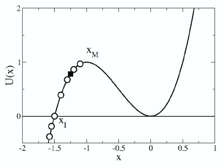
Figure 1: Cubic potential used in the dynamical equation for the variable $x(t)$. The points evidenced in the figure indicate the starting positions $x_{0}$ used for the simulations illustrated in section III (white circles) and section IV (black square).

Let us call $x_{M}$ the abscissa of the potential maximum and $x_{I}$ the cross point between the potential and the $x$ axes. The intervals $x_{o}<x_{I}$ and $I=[x_{I},x_{M}]$ are clearly regions of instability for the system. In systems with a metastable state, the random fluctuations can originate the noise enhanced stability (NES) phenomenon, an interesting effect that increases the stability, enhancing the lifetime of the metastable state NES ; Nes-theory . The mean escape time $\tau$ for a Brownian particle moving throughout a barrier $\Delta U$ is given by the the well known exponential Kramers law Gardiner ; Hanggi

$$\tau=Cexp\left[{\frac{\Delta U}{v}}\right],$$ (7)

where $\tau$ is a monotonically decreasing function of the noise intensity $v$, and $C$ is a prefactor which depends on the potential profile. This is true only if the random walk starts from initial positions inside the potential well. When the starting position is chosen in the instability region $x_{o}<x_{M}$, $\tau$ exhibits an enhancement behavior, with respect to the deterministic escape time, as a function of $v$. This is the NES effect and it can be explained by considering the barrier ”seen” by the Brownian particle starting at the initial position $x_{0}$, that is $\Delta U_{in}=U(x_{max})-U(x_{0})$. Moreover $\Delta U_{in}$ is less than $\Delta U$ as long as the starting position $x_{0}$ lies into the interval $I=[x_{I},x_{M}]$. Therefore for a Brownian particle starting from an unstable initial position it is more likely to enter into the well than to escape from, once the particle has entered. So a small amount of noise can increase the lifetime of the metastable state. For a detailed discussion on this point and different dynamical regimes see Refs. Nes-theory . When the noise intensity $v$ is much greater than $\Delta U$, the Kramers behavior is recovered.
We have already investigated the statistical properties of the escape times for models with stochastic volatility, namely the Heston model and the GARCH model BonannoFNL . We found that the probability density function of the escape times obtained in the Heston model exhibits a better agreement with real data than that calculated in the GARCH model. Here, by considering the modified Heston model (Eqs. (5) and (6)), characterized by a stochastic volatility and a nonlinear Langevin equation for the returns, we study the mean escape time as a function of the model parameters $a$, $b$ and $c$. In particular we investigate whether it is possible to observe some kind of nonmonotonic behavior such that observed for $\tau~{}vs.~{}v$ in the NES effect with constant volatility $v$. We find a nonmonotonic behavior of the mean escape time (MET), $\tau$, as a function of the model parameters. Within this behaviour we recognize the enhancement of $\tau$ as a NES effect in a broad sense.
Our modified Heston model has two limit regimes, corresponding to the cases $a=0$, with only the noise term in the equation for the volatility $v(t)$, and $c=0$ with only the reverting term in the same equation. This last case corresponds to the usual parametric constant volatility regime. In fact, apart from an exponential transient, the volatility reaches the asymptotic value $b$. The NES effect should be observable in the latter case as a function of $b$, which is the average volatility. In fact, in this case we recover the motion of a Brownian particle in a fixed cubic potential with a metastable state and an enhancement of its lifetime for particular initial conditions.
For this purpose we perform simulations by integrating numerically the equations (5) and (6) using a time step $\Delta t=0.01$, and, as potential parameters, $A=2.0$ and $B=3.0$. All the integration steps yielding negative values for $v$ were rejected and repeated. The simulations were performed placing the walker in the initial positions $x_{0}$ located in the unstable region $[x_{I},x_{M}]$ (see Fig. 1) and using an absorbing barrier at $x=-6.0$. Each time the walker hits the barrier, the escape time is registered and another simulation starts, placing the walker at the same initial position $x_{0}$, but using the volatility value of the barrier hitting time.

III Limit cases

First of all we present the result obtained in the limit cases where we have only one of the two terms in the CIR equation (6). Namely: (a) only the reverting term ($a\neq 0,b\neq 0,c=0$, revert-only case), and (b) only the noise term ($a=0$, $b$ whatever, $c\neq 0$, noise-only case) are present. In the case (a) the volatility is practically constant and equal to $b$, apart from an exponential transient that is negligible for times $t\gg a^{-1}$.

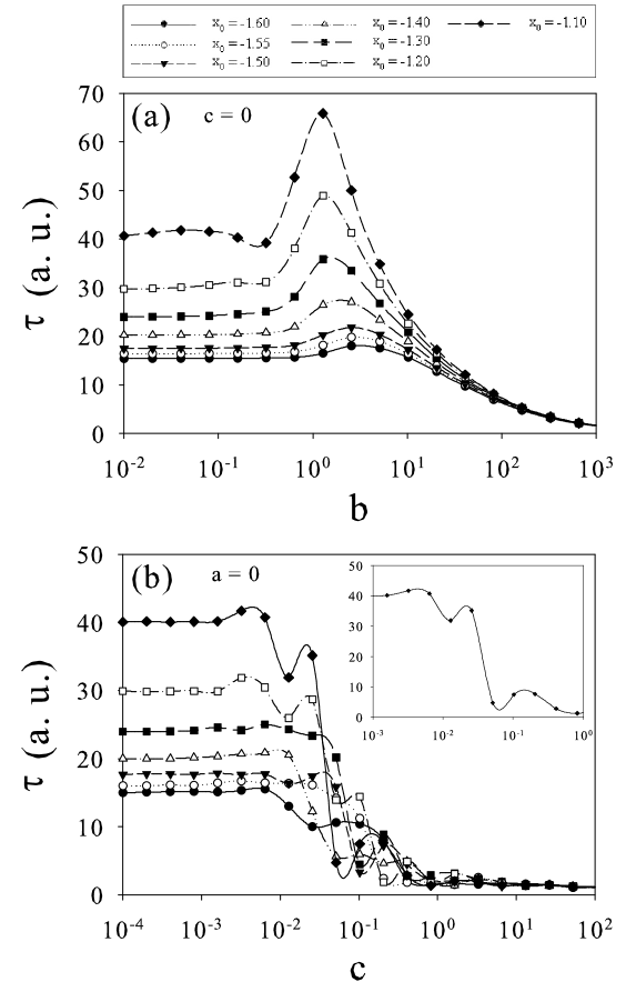
Figure 2: Mean escape time $\tau$ for the seven different starting positions of Fig. 1 (white circles in that figure). Limit cases where only one of the two terms in the CIR equation is present: (a) $\tau$ vs. $b$, when only the reverting term is present ($a=10^{-2}$, $c=0$), and (b) $\tau$ vs. $c$, when only the noise term is present ($a=0$, $b=10^{-2}$). The different starting positions $x_{0}$ from top to bottom are: $-1.1$, $-1.2$, $-1.3$, $-1.4$, $-1.5$, $-1.55$, $-1.60$. The parameters $b$ and $c$ are dimensionless, while $a$, measured in arbitrary units, has dimension of the inverse time. Inset: detail of the curve with $x_{0}=-1.10$.

The mean escape time as a function of $b$ is plotted in Fig. 2a for the seven different initial positions indicated in Fig. 1 (white circles in that figure). The curves are averaged over $10^{5}$ escape events. The nonmonotonic behavior is present. The escape time increases by increasing $b$ until it reaches a maximum. After the maximum, when the values of $b$ are much greater than the potential barrier height, the Kramers behavior is recovered. The nonmonotonic behavior is more evident for starting positions near the maximum of the potential. For starting positions $x_{0}$ lying in the interval $I=[x_{I},x_{M}]$, the initial plateau is an artifact of the calculus. Indeed in the theoretical solution for the constant volatility case, $\tau$ diverges as the noise intensity approaches zero NES ; Nes-theory . With such a noise intensity the escape from the well is a very unlikely event. We should require an infinite number of simulation steps in order to observe an event pushing the particle into the well.

In the case (b), $v$ is a multiplicative stochastic process with standard deviation equal to $c$. The random term in Eq. (6) is given by the product of the white noise and the square root of the process itself $v$. In Fig. 2b we plot $\tau$ as a function of the parameter $c$. The nonmonotonic behavior is absent and the MET decreases monotonically, but differently from the Kramers behavior. The curves are averaged over $10^{8}$ escape events. In this case a greater number of events is required to eliminate the fluctuations present in the curves. Once again we cannot draw any conclusions for the constant behavior of $\tau$, when the values of the parameter $c$ are very small, because of the finite number of simulation steps Nes-theory . It is worthwhile pointing out that the NES effect is not observable as a function of the parameter $c$, if $a=0$. Therefore, the presence of the reverting term affects the behavior of $\tau$ in the domain of the noise term of the volatility and it regulates the transition from nonmonotonic to monotonic regimes of MET. Moreover in this noise-only regime the volatility is proportional to the square of the Wiener process and therefore the fluctuations during the monotonic decreasing behavior of $\tau$ are very large. We see three different dynamical regimes: (i) for low values of the parameter $c$, with respect to the height of the potential barrier, we have a constant behavior, (ii) for intermediate values of $c$ we have fluctuations with decreasing monotonic behavior, (iii) for values of $c$ greater than $1$, which is exactly the height of the barrier, we get very small and constant values of $\tau$ close to zero. This behavior is mainly due to the presence of the Ito term in Eq. (5) for the log-returns $x(t)$. In fact, because of this term we have a fluctuating potential, obtained by the previous one by adding a linear term: $U^{{}^{\prime}}=U(x)+(xv)/2$. The effect of the positive linear term is to modify randomly the potential shape in such a way that the potential barrier disappears for greater values of the volatility $v(t)$. Specifically for values of $v<3$ the potential barrier is always present, while for $v>3$ it disappears. This produces a random enhancement of the escape process with a consequent decreasing behavior of the average escape time.

IV Generic case

In order to present our results for the generic case, where both the reverting and noise terms of the CIR equation are present, we focus on a single starting position, $x_{0}=-1.25$, which is located in the middle of the interval $[x_{I},x_{M}]$. We analyze the escape time through the barrier using different values for parameters $a$, $b$ and $c$. We note that the average escape time $\tau$ is measured in arbitrary units (a. u.), the parameter $a$ (measured in a.u. too) has the dimension of the inverse time, while $b$ and $c$ are dimensionless.

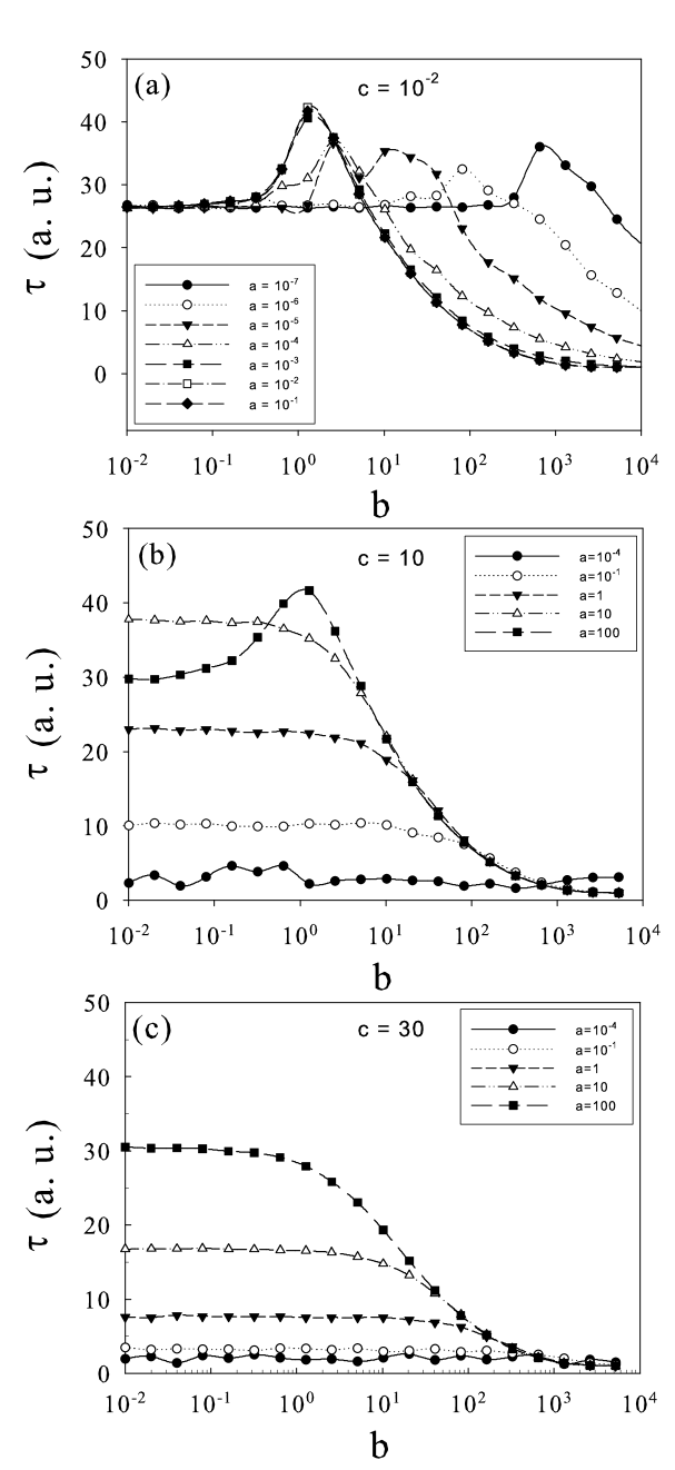
Figure 3: Mean escape time $\tau$ as a function of reverting level $b$. Each panel corresponds to a different value of $c$, specifically (a) $c=10^{-2}$, (b) $c=10$ and (c) $c=30$. Inside each panel different curves correspond to the following values of $a$: (a) black circle $10^{-7}$, white circle $10^{-6}$, black triangle down $10^{-5}$, white triangle up $10^{-4}$, black square $10^{-3}$, white square $10^{-2}$, black diamond $10^{-1}$; (b) and (c) black circle $10^{-4}$, white circle $10^{-1}$, black triangle down $1$, white triangle up $10$, black square $10^{2}$.

As a first result we present the behavior observed for $\tau$ as a function of the reverting level $b$. In Fig. 3 we show the curves averaged over $10^{5}$ escape events. Each panel corresponds to a different value of $c$. Inside each panel different curves correspond to different values of $a$ spanning seven orders of magnitude. The nonmonotonic shape, characteristic of the NES effect, is clearly shown in Fig. 3a. This behavior is shifted towards higher values of $b$ as the parameter $a$ decreases, and it is always present. In Fig. 3c, which corresponds to a much greater value of $c$ ($c=30$), all the curves are monotonic but with a large plateau. So an increase in the value of $c$ causes the NES effect to disappear.

To understand this behavior let us note that the parameters $a$ and $c$ play a regulatory role in Eq. (6). For $a\gg c$ the drift term is predominant while for $a\ll c$ the dynamics is driven by the noise term, unless the parameter $b$ takes great values. In fact in Fig. 3a the nonmonotonic behavior is observed for $a\ll c$, provided that $b\gg c$. For increasing values of $a$ the system approaches the revert-only regime and we recover the behavior shown in Fig. 2a. For $a\ll c$ the shape of the curves changes. The mean escape time $\tau$ is almost constant, and only for very high values of $b$ we observe a decreasing behavior. This happens because for smaller values of $a$ the reverting term becomes negligible in comparison with the noise term and the dependence on $b$ becomes weaker. Only when $b$ is large enough the reverting term assumes values that are no more negligible with respect to the noise term and we can observe again a dependence of $\tau$ on $b$. By increasing the value of $c$ we observe the nonmonotonic behavior only for a very great value of the parameter $a$, that is for $a=100\gg c$ (see Fig. 3b). For further increase of parameter $c$ (see Fig. 3c), the noise experienced by the system is much greater than the effective potential barrier ”seen” by the fictitious Brownian particle and the NES effect is never observable. Moreover we are near a noise-only regime, and we can say that the magnitude of $c$ is so high as to saturate the system.

In summary the NES effect can be observed as a function of the volatility reverting level $b$, the effect being modulated by the parameter $(ab)/c$. The phenomenon disappears if the noise term is predominant in comparison with the reverting term. Moreover the effect is no more observable if the parameter $c$ pushes the system towards a too noisy region.

As a second step we study the dependence of $\tau$ on the noise intensity $c$.

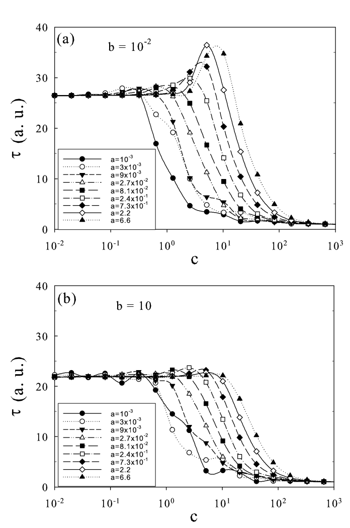
Figure 4: Mean escape time $\tau$ as a function of the noise intensity $c$. Each panel corresponds to a different value of $b$, specifically (a) $b=10^{-2}$ and (b) $b=10$. Inside each panel different curves correspond to the following values of $a$: black circle $10^{-3}$, white circle $3\times 10^{-3}$, black triangle down $9\times 10^{-3}$, white triangle up $2.7\times 10^{-2}$, black square $8.1\times 10^{-2}$, white square $2.4\times 10^{-1}$, black diamond $7.3\times 10^{-1}$, white diamond $2.2$, black triangle up $6.6$.

Fig. 4 shows the curves of $\tau~{}vs~{}c$, averaged over $10^{5}$ escape events. Each panel corresponds to a different value of $b$. Inside each panel different curves correspond to different values of $a$. The shape of the curves is similar to that observed in Fig. 3. For small $b$ (panel a) we observe a nonmonotonic behavior, while for great $b$ (panel b) the curves are monotonic but with a large plateau. Let us recall the results of Fig. 2b: there was no NES effect in the noise-only case. So for small values of $a$, when the reverting term is negligible, the absence of the nonmonotonic behavior is expected. By increasing $a$ the nonmonotonic behavior is recovered (see Fig. 4a). Once again, if one of the parameter pushes the system into a high noise region, the nonmonotonic behavior disappears (see Fig. 4b). Specifically if $b$ is high, the reverting term drives the system towards values of volatility that are outside the region where the NES effect is observable. Indeed a direct inspection of Fig. 3 shows that the value of $b$ used in Fig. 4b is located after the maximum of $\tau$ for all values of $a$ and $c$.

In summary when the noise term is coupled to the reverting term we observe the NES effect on the variable $c$. The effect disappears if $b$ is so high as to saturate the system.

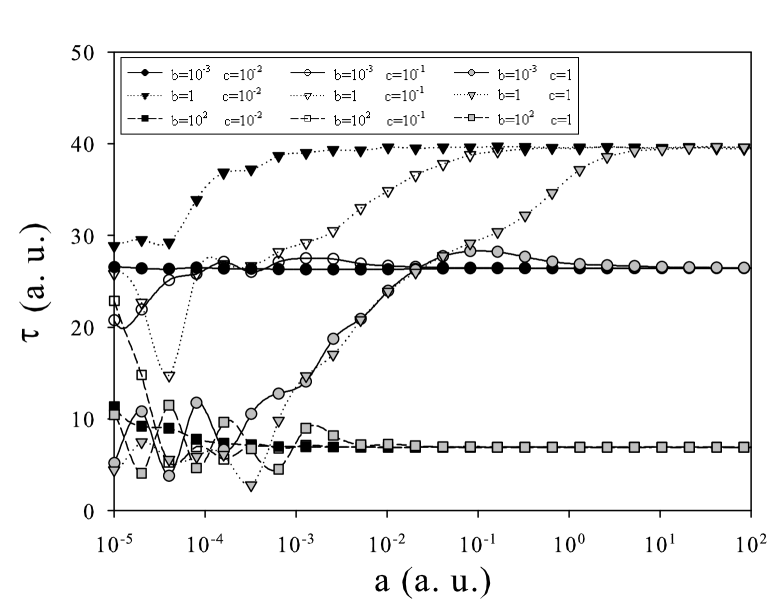
Figure 5: Mean escape time $\tau$ as a function of the reverting rate $a$ for different values of $b$ and $c$. Curves with the same color correspond to the same value of $c$, while curves with the same symbol correspond to the same value of $b$. Specifically the values of $b$ used are: $10^{-3}$ circle, $1$ triangle, $10^{2}$ square . The values of $c$ used are: $10^{-2}$ black, $10^{-1}$ white, $1$ gray.

As a last result we discuss the behavior observed for $\tau$ as a function of the reverting rate $a$. This allow us to observe the transition between the two regimes of the process discussed above: the noise-only regime and the revert-only regime. The results are reported in Fig. 5 for three different values of $b$ and three different values of $c$. To reduce the fluctuations in all the curves when the parameter $a$ becomes small, we performed simulations by averaging on $10^{6}$ escape events. It is worthwhile to note that for values of the parameter $a<10^{-5}$, we enter in the noise-only regime, which characterizes one of the limit cases discussed in section III. Curves with the same color correspond to the same value of $c$ while curves with the same symbol correspond to the same value of $b$.

The system tends to the noise-only regime for lower values of $a$ and to the revert-only regime for higher values of $a$. On the right end of Fig. 5 the curves corresponding to the same value of $b$ tend to group together. The values of $\tau$ the curves approach reflect the nonmonotonic behavior observed in Fig. 3a. Indeed all the curves corresponding to the intermediate value of $b$ ($b=1$) approach a value of $\tau$, which almost corresponds to the maximum value of MET in Fig. 3a (we note that the behavior for $a=10^{-1}$ coincides with that for $a=1$, even if it is not reported in Fig. 3a). This value of $\tau$ is greater than that reached by the curves corresponding to other two, lower and greater, values of $b$ ($10^{-3}$ and $10^{2}$ respectively). Conversely on the left end the curves corresponding to the same value of $c$ tend to group together. It is worth noting that in this last case the curves with the highest value of $c$, namely $c=1$, show greater fluctuations as those observed in all the previous cases where the noise term is predominant (see for example Fig. 2b).

It is interesting to show, for our model (Eqs. (5) and (6)), some of the well-established statistical signatures of the financial time series, such as the probability density function (PDF) of the stock price returns, the PDF of the volatility and the return correlation. In Fig. 6 we show the PDF of the returns. To characterize quantitatively this PDF with regard to the width, the asymmetry and the fatness of the distribution, we calculate the mean value $<\Delta x>$, the variance $\sigma_{\Delta x}$, the skewness $\kappa_{3}$, and the kurtosis $\kappa_{4}$. We obtain the following values: $<\Delta x>=-0.162$, $\sigma_{\Delta x}=0.348$, $\kappa_{3}=-1.958$, $\kappa_{4}=5.374$. These statistical quantities clearly show the asymmetry of the distribution and its leptokurtic nature observed in real market data. In fact, the empirical PDF is characterized by a narrow and large maximum, and fat tails in comparison with the Gaussian distribution Man-Stan ; Bouch-Pott . Specifically we note that the value of the kurtosis $\kappa_{4}=5.374$, which gives a measure of the distance between our distribution and a Gaussian one, is of the same order of magnitude of that obtained for $S\&P$ $500$ for daily prices (see Fig.7.2 on page 114 of Ref. Bouch-Pott ).

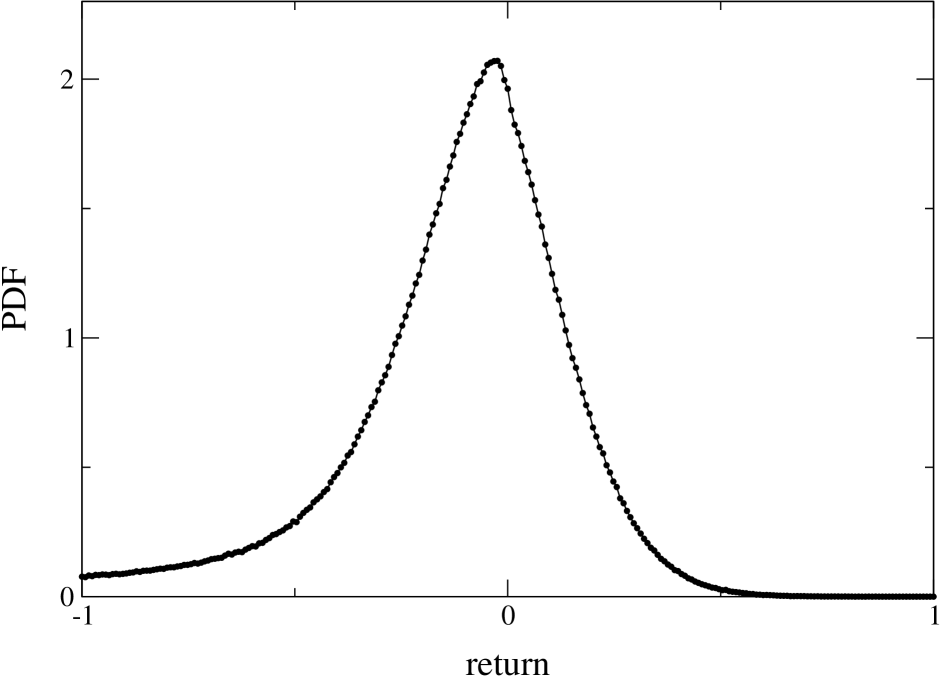
Figure 6: Probability density function of the stock price returns for our model (Eqs. (5) and (6)). The values of the parameters are: $a=10^{-1}$, $b=4.5$, $c=2\times 10^{-1}$. The potential parameters are: $A=2$ and $B=3$.

The presence of the asymmetry is very interesting and it will be subject of future investigations. This asymmetry is due to the nonlinearity introduced in the model through the cubic potential (see Fig. 1). Of course a comparison between the PDF of real data and that obtained from the model requires further investigations on the dynamical behavior of the system, as a function of the model parameters. In the following Fig. 7 we show the PDF of the volatility for our model, and we can see a log-normal behavior as that observed approximately in real market data.

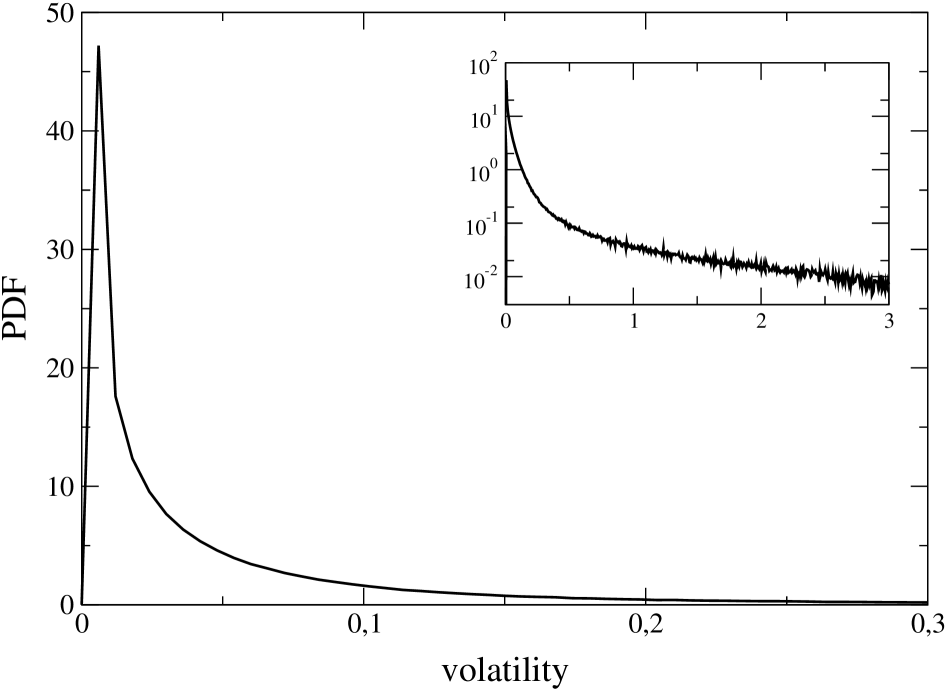
Figure 7: Probability density function of the volatility for our model (Eqs. (5) and (6)). The values of the parameters are the same of Fig. 6. Inset: semilog plot of the PDF of volatility in a longer time scale.

Finally in Fig. 8 we show the correlation function of the returns. As we can see the autocorrelations of the asset returns are insignificant, except for very small time scale for which microstructure effects come into play. This is in agreement with one of the stylized empirical facts emerging from the statistical analysis of price variations in various types of financial markets Cont . A quantitative agreement of the PDF of volatility and the correlation of returns with the corresponding quantities obtained from real market data is subject of further studies.

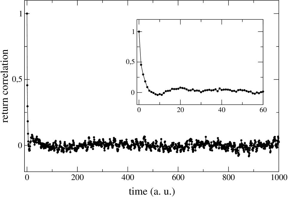
Figure 8: Correlation function of the returns for our model (Eqs. (5) and (6)). The values of the parameters are the same of Fig. 6. Inset: detail of the behaviour at short times.

Our last investigation concerns the PDF of the escape time of the returns, which is the main focus of our paper.

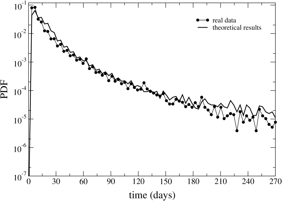
Figure 9: Probability density function of the escape time of the returns from simulation (solid line), and from real data (black circle). The values of the parameters are: $\Delta x_{i}=-0.1\thinspace\sigma_{\Delta x}$, $\Delta x_{f}=-1.0\thinspace\sigma_{\Delta x}$, $x_{0}=-1.25$, $x_{abs}=-6.0$, $v_{start}=8.62\times 10^{-5}$, $a=10^{-1}$, $b=4.5$, $c=2\times 10^{-1}$. The potential parameters are: $A=2$ and $B=3$.

By using our model (Eqs. (5) and (6)), we calculate the probability density function for the escape time of the returns. We define two thresholds, $\Delta x_{i}$ and $\Delta x_{f}$, which represent the start point and the end point for calculating $\tau$ respectively. When the return series reaches the value $\Delta x_{i}$, the simulation starts to count the time $\tau$ and it stops when the threshold $\Delta x_{f}$ is crossed. In order to fix the values of the two thresholds we consider the standard deviation (SD) $\sigma_{\Delta x}$ of the return series over a long time period corresponding to that of the real data. Specifically $\sigma_{\Delta x}$ is the average of the standard deviations $\sigma_{n}$ observed for each stock during the above mentioned whole time period (n is the stock index, varying between $1$ and $1071$). Then we set $\Delta x_{i}=-0.1~{}\sigma_{\Delta x}$ and $\Delta x_{f}=-1.0~{}\sigma_{\Delta x}$. We perform our simulations obtaining a number of time series of the returns equal to the number of stocks considered, which is $1071$. The initial position is $x_{0}=-1.25$ and the absorbing barrier is at $x_{abs}=-6.0$. For the CIR stochastic process $v$, we choose $v_{start}=8.62\times 10^{-5}$, $a=10^{-1}$, $b=4.5$ and $c=2\times 10^{-1}$. The choice of this parameter data set is not based on a fitting procedure as that used for example in Ref. Yakovenko . There the minimization of the mean square deviation between the PDF of the returns, extracted from financial data, and that obtained theoretically is done. We choose the parameter set in the range in which we observe the nonmonotonic behaviour of the mean escape time of the price returns as a function of the parameters $b$ and $c$. Then by a trial and error procedure we select the values of the parameters $a$, $b$, and $c$ for which we obtain the best fitting between the PDF of the escape times calculated from the modified Heston model (Eqs. (5) and (6)) and that obtained from the time series of real market data. We report the results in Fig. 9. Of course a better quantitative fitting procedure could be done, by considering also the potential parameters. This detailed analysis will be done in a forthcoming paper.

As real data we use the daily closure prices for $1071$ stocks traded at the NYSE and continuously present in the $12-$year period $1987-1998$ (3030 trading days). The same data set was used in previous investigations BonannoFNL ; Micci ; Bon_PRE_03 ; Bon_EPJB04 . From this data set we obtain the time series of the returns and we calculate the time to hit a fixed threshold starting from a fixed initial position. The two thresholds were chosen as a fraction of the average standard deviation $\sigma_{\Delta x}$ on the whole time period, as we have done in simulations. The agreement between real data and those obtained from our model is very good. We note that at high escape times the statistical accuracy is worse because of few data with high values. The parameter values of the CIR process for which we obtain good agreement between real and theoretical data are in the range in which we observe the nonmonotonic behavior of MET (see Fig. 3a). This means that in this parameter region we observe a stabilizing effect of the noise on the prices in the time windows for which we have a variation of returns between the two fixed values $\Delta x_{i}$ and $\Delta x_{f}$. This encourages us to extend our analysis to large amounts of financial data and to explore other parameter regions of the model.

V Conclusions

We studied the mean escape time in a market model with a cubic nonlinearity coupled with a stochastic volatility described by the Cox-Ingersoll-Ross equation. In the CIR process the volatility has fluctuations of intensity $c$ and it reverts to a mean level $b$ at rate $a$.

Our results show that as long as the mean level $a$ is different from zero it is possible to observe a nonmonotonic behavior of MET as a function of the two model parameters $b$ and $c$. The parameter $a$ regulates the transition from a noise-only regime, where reverting term is absent or negligible, to a revert-only regime, where the noise term is absent or negligible. In the former case, the enhancement of MET with a nonmonotonic behavior as a function of the model parameters, that is the NES effect, is not observable. The curves have a monotonic shape with a plateau. Moreover, if one of the parameters is so big to push the system into a region where the noise is greater than the barrier height of the effective potential, the effect is no more observable at all. In the revert-only regime, instead, the NES phenomenon is recovered. With its regulatory effect, the reverting rate $a$ can be used to modulate the intensity of the stabilizing effect of the noise observed by varying $b$ and $c$. In this parameter region the probability density function of the escape times of the returns fits very well that obtained from the experimental data extracted by real market.

References

- (1) L. Gammaitoni, P. Hnggi, P. Jung, and F. Marchesoni, Rev. Mod. Phys. 70, 223 (1998); V. S. Anishchenko, A. B. Neiman, F. Moss, and L. Schimansky-Geier, Phys. Usp. 42, 7 (1999); R. N. Mantegna, B.Spagnolo, M. Trapanese, Phys. Rev. E 63, 011101 (2001); T. Wellens, V. Shatokhin, and A. Buchleitner, Rep. Prog. Phys. 67, 45 (2004).
- (2) R. N. Mantegna, B.Spagnolo, Phys. Rev. Lett. 76, 563 (1996); D. Dan, M. C. Mahato and A. M. Jayannavar, Phys. Rev. E 60, 6421 (1999); R. Wackerbauer, Phys. Rev. E 59, 2872 (1999); A. Mielke, Phys. Rev. Lett. 84, 818 (2000); B. Spagnolo, A. A. Dubkov, and N. V. Agudov, Acta Phys. Pol. 35, 1419 (2004).
- (3) N. V. Agudov, B. Spagnolo, Phys. Rev. E 64, 035102(R) (2001); A. Fiasconaro, D. Valenti and B. Spagnolo, Physica A 325, 136 (2003); A. A. Dubkov, N. V. Agudov and B. Spagnolo, Phys. Rev. E 69, 061103 (2004); A. Fiasconaro, B. Spagnolo and S. Boccaletti, Phys. Rev. E 72, 061110(5) (2005).
- (4) G. Parisi, Nature 433, 221(2005); H. Larralde and F. Leyvraz, Phys. Rev. Lett. 94, 160201 (2005); C. M. Dobson, Nature 426, 884 (2003); M. Acar, A. Becskei, and A. van Oudenaarden, Nature 435, 228 (2005); C. Lee et al., Nature Reviews Molecular Cell Biology 5, 7 (2004).
- (5) A.L. Pankratov and B. Spagnolo, Phys. Rev. Lett. 93, 177001 (2004); H. Larralde and F. Leyvraz, Phys. Rev. Lett. 94, 160201 (2005); E. V. Pankratova, A. V. Polovinkin, and B. Spagnolo, Phys. Lett. A 344, 43 (2005).
- (6) P.W. Anderson, K.J. Arrow and D. Pines, The economy as an evolving complex system, (Addison Wesley Longman, XX, 1988); P.W. Anderson, K.J. Arrow, and D. Pines, The economy as an evolving complex system II, (Addison Wesley Longman, XX, 1997).
- (7) R.N. Mantegna and H.E. Stanley An introduction to econophysics: correlations and complexity in finance, (Cambridge University Press, Cambridge, 2000).
- (8) J.-P. Bouchaud and M. Potters Theory of financial risks, (Cambridge University Press, Cambridge, 2000).
- (9) R. Cont, Quantitative Finance 1, 223 (2001).
- (10) L. Bachelier Théorie de la spéculation [Ph.D. Thesis], Annales scientifiques de l’ecole normale supérieure III-17, 21–86 (1900).
- (11) M.M. Dacorogna, R. Gencay, U.A. Müller, R.B. Olsen and O.V. Pictet An Introduction to High-Frequency Finance, (Academic Press, New York, 2001).
- (12) S.L. Heston, Rev. Financial Studies 6, 327 (1993).
- (13) J. Cox, J. Ingersoll, and S. Ross, Econometrica 53, 385 (1985); J.P. Fouque, G. Papanicolau and K.R. Sircar Derivatives in financial markets with stochastic volatility, (Cambridge University Press, Cambridge, 2000).
- (14) W. Feller, Ann. Math. 54, 173 (1951).
- (15) A. Christian Silva, Richard E. Prange, Victor M. Yakovenko, Physica A 344, 227 (2004); A. Christian Silva, Application of Physics to Finance and Economics: Returns, Trading Activity and Income, arXiv:cond-mat/0507022 (2005).
- (16) G. Bonanno and B. Spagnolo, Fluctuation and Noise Letters 5, L325 (2005); Stochastic Models and Escape Times of Financial Markets, Mod. Probl. Stat. Phys. 4, 122 (2005).
- (17) S. Miccichè, G. Bonanno, F. Lillo and R.N. Mantegna, Physica A 314, 756 (2002).
- (18) A.A. Dragulescu and V.M. Yakovenko, Quantitative Finance 2, 443 (2002).
- (19) Y. Louzoun. and S. Solomon, Physica A 302, 220 (2001); S. Solomon and P. Richmond, Eur. Phys. J. B 27, 257 (2002); O. Malcai, O. Biham, P. Richmond, and S. Solomon, Phys. Rev. E 66, 031102 (2002).
- (20) L. Borland, Phys. Rev. E 57, 6634 (1998); Quantitative Finance 2, 415 (2002).
- (21) L. Borland, Phys. Rev. Lett. 89, 098701 (2002).
- (22) P. Neu and R. Khn, Physica A 342, 639 (2004); J. P. L. Hatchett and R. Khn, J. Phys. A: Math. Gen. 39, 2231 (2006).
- (23) J.-P. Bouchaud and R. Cont, Eur. Phys. J. B 6, 543 (1998).
- (24) J.-P. Bouchaud, Quantitative Finance 1, 105 (2001).
- (25) J.-P. Bouchaud, Physica A 313, 238 (2002).
- (26) D. Sornette, Physics Reports 378, 1, (2003).
- (27) B.M. Friedman, D.I. Laibson, H.P. Minsky, Brooking papers on economic activity 1989, 137 (1989).
- (28) J. Masoliver, M. Montero, and J. Perell, Phys. Rev. E 71, 056130 (2005).
- (29) M. Montero, J. Perell, J. Masoliver, F. Lillo, S. Miccich, and R. N. Mantegna, Phys. Rev. E 72, 056101 (2005).
- (30) E. Scalas, R. Gorenflo, F. Mainardi, Physica A 284, 376 (2000); F. Mainardi, M. Raberto, R. Gorenflo, and E. Scalas, Physica A 287, 468 (2000); M. Raberto, E. Scalas, and F. Mainardi, Physica A 314, 749 (2002); E. Scalas, Five Years of Continuous-time Random Walks in Econophysics, arXiv:cond-mat/0501261 (2005).
- (31) C. W. Gardiner Handbook of Stochastic Methods, (Springer, Berlin, 2004).
- (32) P. Hnggi, P. Talkner and M. Borkovec, Rev. Mod. Phys. 62, 251 (1990); E. Pollak and P. Talkner, Chaos 15, 026116 (2005).
- (33) G. Bonanno, G. Caldarelli, F. Lillo, and Rosario N. Mantegna, Phys. Rev. E 68, 046130 (2003).
- (34) G. Bonanno, G. Caldarelli, F. Lillo, S. Miccichè, N. Vandewalle, and R. N. Mantegna, Eur. Phys. J. B 38, 363 (2004).