On the number of contacts of a floating polymer chain crosslinked with a surface adsorbed chain on fractal structures

Abstract

We study the interaction problem of a linear polymer chain, floating in fractal containers that belong to the three-dimensional Sierpinski gasket (3D SG) family of fractals, with a surface-adsorbed linear polymer chain. Each member of the 3D SG fractal family has a fractal impenetrable 2D adsorbing surface, which appears to be 2D SG fractal. The two-polymer system is modelled by two mutually crossing self-avoiding walks. By applying the Monte Carlo Renormalization Group (MCRG) method, we calculate the critical exponents $\varphi$, associated with the number of contacts of the 3D SG floating polymer chain, and the 2D SG adsorbed polymer chain, for a sequence of SG fractals with $2\leq b\leq 40$. Besides, we propose the codimension additivity (CA) argument formula for $\varphi$, and compare its predictions with our reliable set of the MCRG data. We find that $\varphi$ monotonically decreases with increasing $b$, that is, with increase of the container fractal dimension. Finally, we discuss the relations between different contact exponents, and analyze their possible behaviour in the fractal-to-Euclidean crossover region $b\to\infty$.

1 Introduction

The self-avoiding walk (SAW) is a random walk that must not contain self-intersections. This kind of random walk, placed on a lattice, has been widely used as a model of a linear polymer in a good solvent [1]. Even though an isolated polymer chain is difficult to observe experimentally, numerous studies of the single-chain statistics have been upheld as a requisite step towards understanding the statistics of collection-chain systems [2]. A reasonable extension of a single polymer concept is a model of two interacting linear polymers (two interacting SAWs), which has been a subject of extensive studies because of its theoretical and practical interest. To investigate the critical properties of the two-chain (or many-chain) systems various theoretical techniques have been applied, including the field theoretical approach [3], Monte Carlo simulations [4, 5], transfer-matrix calculations [6], and renormalization group (RG) methods [7, 8, 9]. Among other fields, a system of two interacting SAWs, that are mutually avoiding, has been successfully applied as a model of diblock copolymers [10, 11], as well as in the studies of double-stranded DNA molecules [12, 13, 14].

In order to study the number of contacts between monomers that belong to different polymers, the two-polymer system may be modelled by two mutually crossing self-avoiding walks [15, 16], that is, by two SAWs whose paths on an underlying lattice can cross (intersect) each other. Each crossing between two SAW paths corresponds to a contact of two monomers that belong to different polymer chains, and therefore with each crossing we may associate the contact energy $\epsilon_{c}$. In analogy with the problem of polymer adsorption onto a hyperplane [17], we may assume that with decreasing of temperature the number of crossings $M$ increases so that at the critical temperature $T_{c}$ it behaves according to the power law

$$M\sim N^{\varphi}\>,$$ (1)

where $N$ is the total number of monomers in the longer chain, and $\varphi$ is the crossover critical exponent. Below $T_{c}$ the number of contacts becomes proportional to $N$, whereas above $T_{c}$ it is vanishingly small.

In spite of different approaches to the two-SAW problem, the entire physical picture achieved so far, is almost entirely of a phenomenological character and there are only few numerical results. For instance, in the case of Euclidean lattices, besides the codimension additivity (CA) argument predictions for the contact critical exponents (with conjectures $\varphi=1/2$ in $d=2$, and $\varphi\approx 1/5$ in $d=3$), there is only Monte Carlo result $\varphi=0.516\pm 0.005$, for a model of two mutually crossing SAWs on the square lattice [16]. The above problem has been also studied on fractal lattices. But, in the case of fractals it may be noted that the two-dimensional (2D) fractal lattices (embedded in the 2D Euclidean space) have been more frequently investigated [15, 18, 19] than the corresponding model in the case of 3D fractal structures [20]. Since the 3D fractals definitely may serve as a better description of real systems (porous media, for instance), it is recommendable to study the described model in a case of a set of 3D fractals. For this reason, it is desirable to extend the study of two-polymer system on a family of fractal lattices whose characteristics approach properties of a 3D Euclidean lattice.

In this paper we report results of our study for the contact critical exponent $\varphi$ of two polymer chains, that display inter-chain interactions, in the three-dimensional fractal lattices that belong to the Sierpinski gasket (SG) family of fractals. The two-polymer system is modelled by two SAWs which are allowed to cross each other. We assume that the first polymer is a floating chain in the bulk of 3D SG fractal, while the second polymer chain is adsorbed onto one of the four surfaces (which is, in fact, 2D SG fractal) by which is 3D SG fractal bounded. In section 2 of the paper, we first describe the 3D SG fractals for general $b$. Then, we present the framework of the RG method for studying statistics of two mutually crossing SAW chains, taking into account the presence of the inter-chain interactions, in a way that should make the method transparent for the Monte Carlo calculations of the contact critical exponent $\varphi$. In section 3 we present the obtained specific values of $\varphi$ for a sequence of 3D SG fractals, that is, for $2\leq b\leq 40$. In the same section we propose the phenomenological formulae for $\varphi$, based on the CA arguments, test their predictions on the obtained MCRG data, and discuss relations between different contact exponents. Summary of the obtained results and the relevant conclusions are given in section 4.

2 Monte Carlo renormalization group approach

In this section we are going to apply the Monte Carlo renormalization group (MCRG) method to the studied model of interacting polymers on the 3D SG family of fractals. These fractals have been studied in numerous papers so far, and consequently we shall give here only a requisite brief account of their basic properties. It starts with recalling the fact that each member of the 3D SG fractal family is labelled by an integer $b\geq 2$ and can be constructed in stages. At the first stage ($r=1$) of the construction there is a tetrahedron of base $b$ that contains $b(b+1)(b+2)/6$ upward oriented unit tetrahedrons. The subsequent fractal stages are constructed recursively, so that the complete self-similar fractal lattice can be obtained as the result of an infinite iterative process of successive $(r\to r+1)$ enlarging the fractal structure $b$ times, and replacing the smallest parts of enlarged structure with the initial structure $r=1$ (see for instance, figure 1 of [21]). Fractal dimension $d_{f}$ of the 3D SG fractal is equal to

$$d_{f}^{3D}={{\ln[{{b(b+1)(b+2)}/6}}]/{\ln b}}\>.$$ (2)

We assume here that one of the four boundaries of the 3D SG fractal is an impenetrable adsorbing surface, which is itself a 2D SG fractal with the fractal dimension

$$d_{f}^{2D}=\ln[b(b+1)/2]/\ln b\>.$$ (3)

In the terminology that applies to the SAW, we assign the weight $x_{3}$ to a step of the SAW in the bulk (3D SG fractal), which represents a floating polymer (we mark it by $P_{3}$), and the weight $x_{2}$ to a step of the SAW adsorbed on the surface (2D SG fractal), which represents an adsorbed polymer (marked by $P_{2}$), whose monomers act as pining cites for the floating polymer. In order to explore interacting effects of two SAWs on the underlying fractals, we introduce the two Boltzmann factors $w=e^{-\epsilon_{c}/k_{B}T}$ and $t=e^{-\epsilon_{t}/k_{B}T}$, where $\epsilon_{c}$ is the energy of two monomers in contact (which occurs at a crossing site of SAWs), while $\epsilon_{t}$ is the energy associated with two sites which are nearest neighbours to a crrosslinked site and which are visited by different SAWs (see figure 1).

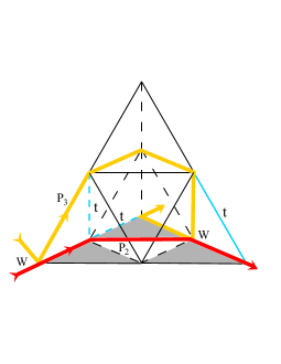
Figure 1: The structure of the three-dimensional SG fractal, for $b=2$, at the first stage of construction, with an example of the bulk polymer chain ($P_{3}$) depicted by yellow line and the surface-adsorbed polymer chain ($P_{2}$) depicted by red line. The shaded area represents the adsorbing surface (the two-dimensional SG fractal). The two polymers are crosslinked at the two cites, so that each contact contributes the weight factors $w$. The blue bonds, marked by $t$, describe the interactions between those monomers which are nearest neighbors to the crosslinked points. Thus, the depicted two-polymer configuration contributes the weight $x_{3}^{5}x_{2}^{3}w^{2}t^{3}$ in the corresponding RG equation (especially, in the equation (7) for $i=2$ and $r=0$).

To describe all possible configurations of the two-chain polymer system, within the accepted model, we need to introduce the nine restricted partition functions $A^{(r)}$, $B^{(r)}$, $C^{(r)}$, $A_{i}^{(r)}\,(i=1,2,3,4)$, and $B_{i}^{(r)}\,(i=1,2)$, that are depicted in figure 2. The recursive nature of the fractal construction implies the following recursion relations for restricted partition functions

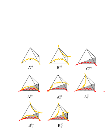
Figure 2: Schematic representation of the nine restricted generating functions used in the description of all possible two-SAW configurations, within the $r$-th stage of the 3D SG fractal structure. Thus, for example, the $A_{1}^{(r)}$ represents the configuration when both polymers (3D SG floating and 2D SG adsorbed) pass through the same vertices of a particular $r$-th stage of the fractal lattice. The interior details of the $r$-th stage fractal structure, as well as details of the chains, are not shown (for the chains, they are manifested by the wiggles of the SAW paths).

$$A^{(r+1)}=\sum_{N_{A},N_{B}}a(N_{A},N_{B})\,A^{N_{A}}B^{N_{B}}\,,$$ (4)

$$B^{(r+1)}=\sum_{N_{A},N_{B}}b(N_{A},N_{B})\,A^{N_{A}}B^{N_{B}}\,,$$ (5)

$$C^{(r+1)}=\sum_{N_{C}}c(N_{C})\,C^{N_{C}}\,,$$ (6)

$$A_{i}^{(r+1)}=\sum_{\cal{N}}a_{i}({\cal{N}})\,A^{N_{A}}B^{N_{B}}C^{N_{C}}\prod_{j=1}^{4}A_{j}^{N_{A_{j}}}\prod_{k=1}^{2}B_{k}^{N_{B_{k}}}\,,\quad i=1,2,3,4\>,$$ (7)

$$B_{i}^{(r+1)}=\sum_{\cal{N}}b_{i}({\cal{N}})\,A^{N_{A}}B^{N_{B}}C^{N_{C}}\prod_{j=1}^{4}A_{j}^{N_{A_{j}}}\prod_{k=1}^{2}B_{k}^{N_{B_{k}}}\,,\quad i=1,2\>,$$ (8)

where $\cal{N}$ denotes the set of numbers ${\cal{N}}=\{N_{A},N_{B},N_{C},N_{A_{1}},N_{A_{2}},N_{A_{3}},N_{A_{4}},N_{B_{1}},N_{B_{2}}\}$, and, where we have omitted the superscript $(r)$ on the right-hand side of the above relations. The self-similarity of the fractals implies that the sets of coefficients $a,b$ and $c$, that describe a single polymer configurations ($a$ and $b$ coefficients describe the bulk polymer configurations, whereas the $c$ coefficients describe the adsorbed polymer configurations), and the sets of coefficients $a_{i}$ and $b_{i}$ of the corresponding two-chain configurations do not depend on $r$. Each of the two-chain coefficients ($a_{i}$ and $b_{i}$) represents the number of ways in which the corresponding parts of the two-SAW configuration, within the $(r+1)$-th stage fractal structure, can be comprised of the two-SAW configurations within the fractal structures of the next lower order. Because of the independence of $r$, these coefficients can be calculated by studying all two-SAW paths within the fractal generator only, that is on the first step of construction $r=1$.

The above set of relations (4)–(8), can be considered as the RG equations for the problem under study, with the initial conditions: $A^{(0)}=x_{3}$, $B^{(0)}=x_{3}^{2}$, $C^{(0)}=x_{2}$, $A_{1}^{(0)}=x_{3}x_{2}w^{2}$, $A_{2}^{(0)}=A_{3}^{(0)}=x_{3}x_{2}wt$, $A_{4}^{(0)}=x_{3}x_{2}$ and $B_{1}^{(0)}=B_{2}^{(0)}=x_{3}^{2}x_{2}w^{2}$, which correspond to the unit tetrahedron. On the physical grounds that are reasonable for the studied model [22], one can expect that the RG transformations should have three relevant fixed points of the general type

$$(A^{*},B^{*},C^{*},A_{1}^{*},A_{2}^{*},A_{3}^{*},A_{4}^{*},B_{1}^{*},B_{2}^{*}).$$ (9)

The first fixed point

$$(A^{*},B^{*},C^{*},0,0,0,A_{4}^{*},0,0),$$ (10)

with $A_{i}^{*}=0\,(i=1,2,3)$, $A_{4}^{*}=A_{4}^{*}(A^{*},B^{*},C^{*})$ and $B_{i}^{*}=0\,(i=1,2)$, due to the meaning of these quantities (see figure 2), describes segregated phase of two chain polymers that should be expected in the high temperature region $T>T_{c}$. The second fixed point

$$(A^{*},B^{*},C^{*},A^{*}C^{*},A^{*}C^{*},A^{*}C^{*},A^{*}C^{*},B^{*}C^{*},B^{*}C^{*}),$$ (11)

with $A_{i}^{*}=A^{*}C^{*}\,(i=1,2,3,4)$ and $B_{i}^{*}=B^{*}C^{*}\,(i=1,2)$, which appears to be a tricritical point, describes the state of the two-polymer system that occurs at the critical temperature $T=T_{c}$ when segregated and entangled polymer phases become identical. Finally, the third fixed point

$$(0,0,0,C^{*},0,0,0,0,0),$$ (12)

with the nonzero value only for $A_{1}^{*}=C^{*}$, describes the polymer entangled state, which should appear at low temperatures $T<T_{c}$.

In what follows we focus our attention on the tricritical fixed point (11) to calculate the contact critical exponent $\varphi_{32}$ between $P_{3}$ and $P_{2}$ polymer chains. We can observe that the above system of RG equations (4)–(8) can be split into three uncoupled sets of RG equations: (4)–(5), (6), and (7)–(8). Moreover, it should be noticed, that for each $b$, the first two sets of RG equations, (4)–(5) and (6), have only one nontrivial fixed point value $(A^{*},B^{*})$ [21] and $C^{*}$ [23] respectively, which thereby completely determine the coordinates of the tricritical fixed point. Calculation of $\varphi_{32}$ starts with solving the eigenvalue problem of the RG equations (4)–(8), linearized at the tricritical fixed point. The related eigenvalue problem can be separated into three parts. The first part of the eigenvalue problem, related to the equations (4)–(5) gives the eigenvalue $\lambda_{\nu_{3}}$ of the end–to–end distance critical exponent $\nu_{3}=\ln b/\ln\lambda_{\nu_{3}}$ of the 3D SG floating polymer, while the second part, related to the equation (6), gives the eigenvalue $\lambda_{\nu_{2}}$ of the end–to–end distance critical exponent $\nu_{2}=\ln b/\ln\lambda_{\nu_{2}}$ of the 2D SG SAW, that represents the adsorbed polymer. Finally, the third part of the eigenvalue problem (related to the equations (7)–(8)) reduces to solving the equation

$$\mbox{det}\left|\left({\partial X^{\prime}_{i}\over\partial X_{j}}\right)^{*}-\lambda\,\delta_{ij}\right|=0,$$ (13)

where $X_{i}$ are elements of the set $\{A_{1},A_{2},A_{3},A_{4},B_{1},B_{2}\}$, and the asterisk means that the derivatives should be taken at the tricritical fixed point. Also, we have used the prime symbol as a superscript for the $(r+1)$–th restricted partition functions and no indices for the $r$–th order partition functions. The largest eigenvalue $\lambda_{\varphi_{32}}$ of above equation determines the contact critical exponent via the formula

$$\varphi_{32}={\ln{\lambda_{\varphi_{32}}}\over\ln\lambda_{\nu_{3}}}.$$ (14)

Hence, in an exact RG evaluation of $\varphi_{32}$ one needs to calculate partial derivatives of sums (4)–(8), and thereby one should find the coefficients $a,b,c,a_{i}$, and $b_{i}$. The latter can be calculated by an exact enumeration of all possible two-SAW configurations for each particular $b$. We have found that this enumeration is feasible only for small $b$. However, for large $b$ the exact enumeration turns out to be a forbidding task. We bypass this problem by applying the MCRG method. Within this method, the first step would be to locate the tricritical fixed point. To this end, we may observe that the results obtained in [21] provide information for both $(A^{*},B^{*})$ and $\lambda_{\nu_{3}}$ for a sequence of 3D SG fractals with $2\leq b\leq 40$, whereas the results obtained in [24] give the fixed point values of $C^{*}$ for 2D SG fractals, for $b$ in the range $2\leq b\leq 80$ . Accordingly, the next step in the MCRG method consists of finding $\lambda_{\varphi_{32}}$ without explicit calculation of the RG equation coefficients.

To solve the partial eigenvalue problem (13), so as to learn $\lambda_{\varphi_{32}}$, we need to find the requisite 36 partial derivatives. These derivatives can be related to various averages of the numbers $N_{A_{i}}$ and $N_{B_{i}}$ of different crossings of the SAWs for various two–SAW configurations that correspond to the restricted partition functions $A_{i}^{(r)}$ and $B_{i}^{(r)}$. For instance, starting with (7) (in the notation that does not use the superscripts $(r+1)$ and $r$) and by differentiating it with respect to $A_{1}$ we get

$${\partial{A_{i}^{\prime}}\over\partial{A_{1}}}=\sum_{\cal{N}}N_{A_{1}}a_{i}({\cal{N}})\,A^{N_{A}}B^{N_{B}}C^{N_{C}}A_{1}^{-1}\prod_{j=1}^{4}A_{j}^{N_{A_{j}}}\prod_{k=1}^{2}B_{k}^{N_{B_{k}}}\,,\quad i=1,2,3,4\>.$$ (15)

Now, assuming that $A_{i}^{\prime}$ represents the grand canonical partition functions for the ensemble of all possible two-SAW configurations, where each of two SAWs starts and leaves fractal generator at two fixed corners, so that the first SAW is a 3D SG floating chain, while the other SAW is a 2D SG adsorbed chain. With this concept in mind, we can write the corresponding ensemble average

$${\langle N_{A_{1}}\rangle}_{A_{i}^{\prime}}={1\over A_{i}^{\prime}}\sum_{\cal{N}}N_{A_{1}}a_{i}({\cal{N}})\,A^{N_{A}}B^{N_{B}}C^{N_{C}}\prod_{j=1}^{4}A_{j}^{N_{A_{j}}}\prod_{k=1}^{2}B_{k}^{N_{B_{k}}}\,,\quad i=1,2,3,4\>,$$ (16)

which can be directly measured in a Monte Carlo simulation. Combing (15) and (16) we can express the requisite partial derivative in terms of the measurable quantity

$${\partial{A_{i}^{\prime}}\over\partial{A_{1}}}={A_{i}^{\prime}\over A_{1}}{\langle N_{A_{1}}\rangle}_{A_{i}^{\prime}}\,,\quad i=1,2,3,4\>.$$ (17)

In a similar way we can find the rest derivatives, so that all needed derivatives, calculated in the tricritical fixed point, may be related with the corresponding averages

$${\left({\partial{A_{i}^{\prime}}\over\partial{A_{j}}}\right)}^{*}={\langle N_{A_{j}}\rangle}_{A_{i}^{\prime}}^{*}\>,\quad{\left({\partial{A_{i}^{\prime}}\over\partial{B_{k}}}\right)}^{*}={A^{*}\over B^{*}}{\langle N_{B_{k}}\rangle}_{A_{i}^{\prime}}^{*}\,,\quad i,j=1,2,3,4\>;\>\>k=1,2\>,$$ (18)

$${\left({\partial{B_{l}^{\prime}}\over\partial{A_{j}}}\right)}^{*}={B^{*}\over A^{*}}{\langle N_{A_{j}}\rangle}_{B_{l}^{\prime}}^{*}\>,\quad{\left({\partial{B_{l}^{\prime}}\over\partial{B_{k}}}\right)}^{*}={\langle N_{B_{k}}\rangle}_{B_{l}^{\prime}}^{*}\,,\quad j=1,2,3,4\>;\>\>k,l=1,2\>.$$ (19)

Consequently to solve the eigenvalue problem (13), so as to learn $\lambda_{\varphi_{32}}$, we need to find the above partial derivatives at the tricritical fixed point. These derivatives are related to various averages of the numbers $N_{A_{j}}$, and $N_{B_{k}}$, of different two-SAW parts (of the types $A_{j}$, and $B_{k}$) within the corresponding two-SAW configurations (described with $A^{\prime}_{i}$ or $B^{\prime}_{l}$). Therefore, to calculate the derivatives (18)–(19) at the tricritical fixed point, one needs 36 averages ($\langle N_{A_{j}}\rangle_{A^{\prime}_{i}}^{*}$, $\langle N_{B_{k}}\rangle_{A^{\prime}_{i}}^{*}$, $\langle N_{A_{j}}\rangle_{B^{\prime}_{l}}^{*}$, $\langle N_{B_{k}}\rangle_{B^{\prime}_{l}}^{*}$), which are all measurable through Monte Carlo simulations. The pertinent Monte Carlo technique has been described in [24], and we would not like to elaborate on them here. Solving numerically the eigenvalue equation (13) we obtain $\lambda_{\varphi_{32}}$, and, finally, using relation (14), we calculate the contact critical exponent $\varphi_{32}$, whose specific values we present in the next section.

3 Results and discussion

We have studied the interaction problem of a floating polymer chain confined in the 3D SG fractal container, with a surface (2D SG fractal) adsorbed polymer chain to calculate the critical exponent $\varphi_{32}$ which governs the number of contacts between two chains.

The main goal of this study is the MCRG evaluation of $\varphi_{32}$, for various values of $b$. Furthermore, in the case $b=2$, we have calculated the exact value. To find the exact forms of RG equations (4)–(8), for $b=2$ fractal, using the computer facilities we have been able to enumerate all coefficients (which are available upon request addressed to the author) that appear in these equations. Linearization of obtained RG equations around the tricritical fixed point (11), in this case determined by the values $A^{*}=0.4294$, $B^{*}=0.0499$ and $C^{*}=0.6180$ [25], gives the following eigenvalues: $\lambda_{\nu_{3}}(b=2)=2.7965$ and $\lambda_{\varphi_{32}}(b=2)=1.7475$, whereupon we find the exact value $\varphi_{32}(b=2)=\ln 1.7475/\ln 2.7965=0.5428$. Here, we notice that the same model is studied on the four-simplex lattice, which belongs to the same universality class as the $b=2$ 3D SG fractal. In this study [22] the value $\varphi_{32}=0.5669$ is reported, which appears as an approximate result (and deviates 4% from our exact finding), since in approach applied in [22] some two-SAW configurations are not taken into account (more precisely, the configurations described by function $A_{2}^{(r)}$, in our notation).

Table 1: The MCRG ($2\leq b\leq 40$) results obtained in this work for the contact critical exponents $\varphi_{32}$ for the 3D SG family of fractals. For the completeness we quote here the MCRG values for the RG parameters $(A^{*},B^{*})$ [21], and $C^{*}$ [24].

$b$ $A^{*}$ $B^{*}$ $C^{*}$ $\varphi_{32}$ 2 0.4311$\pm$0.0009 0.0505$\pm$0.0023 0.61825$\pm$0.00061 0.5440$\pm$0.0056 3 0.3421$\pm$0.0004 0.0245$\pm$0.0015 0.55137$\pm$0.00044 0.4969$\pm$0.0024 4 0.2898$\pm$0.0004 0.0122$\pm$0.0020 0.50658$\pm$0.00034 0.4658$\pm$0.0006 5 0.2560$\pm$0.0004 0.0067$\pm$0.0019 0.47455$\pm$0.00028 0.4451$\pm$0.0012 6 0.2319$\pm$0.0003 0.0038$\pm$0.0012 0.45091$\pm$0.00024 0.4250$\pm$0.0004 7 0.2148$\pm$0.0003 0.0020$\pm$0.0018 0.43240$\pm$0.00021 0.4092$\pm$0.0008 8 0.2016$\pm$0.0003 0.0012$\pm$0.0026 0.41780$\pm$0.00019 0.3963$\pm$0.0006 9 0.1912$\pm$0.0004 0.0007$\pm$0.0008 0.40574$\pm$0.00017 0.3841$\pm$0.0007 10 0.1829$\pm$0.0003 0.0005$\pm$0.0023 0.39586$\pm$0.00007 0.3714$\pm$0.0005 12 0.1703$\pm$0.0004 0.0001$\pm$0.0035 0.38037$\pm$0.00013 0.3514$\pm$0.0004 15 0.1581$\pm$0.0001 – 0.36396$\pm$0.00011 0.3226$\pm$0.0003 17 0.1526$\pm$0.0001 – 0.35593$\pm$0.00008 0.3126$\pm$0.0003 20 0.1462$\pm$0.0001 – 0.34681$\pm$0.00006 0.2956$\pm$0.0003 25 0.1399$\pm$0.0001 – 0.33602$\pm$0.00008 0.2677$\pm$0.0003 30 0.1353$\pm$0.0001 – 0.32876$\pm$0.00007 0.2573$\pm$0.0002 35 0.1327$\pm$0.0001 – 0.32350$\pm$0.00008 0.2183$\pm$0.0003 40 0.1305$\pm$0.0001 – 0.31936$\pm$0.00006 0.2016$\pm$0.0003

For larger $b$, that is, for fractals in the range $2\leq b\leq 40$, we have applied the MCRG method expounded in the previous section. The obtained MCRG values for $\varphi_{32}$, together with the pertaining error bars (determined from statistics of measured quantities through the Monte Carlo simulations), are given in table 1. The values of $\varphi_{32}$ for fractals $2\leq b\leq 30$, have been calculated from averages obtained from $10^{6}$ Monte Carlo simulations performed for each possible two-SAW configuration, while $\varphi_{32}$ for fractals $b=35$ and $b=40$ was obtained performing $5\,10^{5}$ Monte Carlo simulations. The time needed to calculate all requisite averages ($\langle N_{A_{j}}\rangle_{A^{\prime}_{i}}^{*}$, $\langle N_{B_{k}}\rangle_{A^{\prime}_{i}}^{*}$, $\langle N_{A_{j}}\rangle_{B^{\prime}_{l}}^{*}$, $\langle N_{B_{k}}\rangle_{B^{\prime}_{l}}^{*}$) increases exponentially with the scale parameter $b$, so that for $5\,10^{5}$ simulations performed on fractals $b=10$ and $b=40$, at the corresponding tricritical fixed points, it was required 10 minutes and 90 hours of the available CPU time, respectively (on a PC with the Intel Pentium 4 processor).

Comparing our MCRG and exact result for $b=2$ fractal ($0.5440\pm 0.0056$ versus $0.5428$) we can see that the MCRG result deviates 0.22% from the exact RG finding, which is a very well agreement between the two (Monte Carlo and exact) approaches of solving the problem, and thereby provides reliance on accuracy of the MCRG results for larger $b$. In figure 3 we depict our MCRG findings for the critical exponent $\varphi_{32}$, of the 3D SG family of fractals, as a function of $1/b$. We observe that the critical exponent $\varphi_{32}$, in the region $2\leq b\leq 40$, is a monotonically decreasing function of $b$, which means that the number of polymer contacts (crossings of the SAW paths) decreases with increasing of the fractal dimension of the SG fractals.

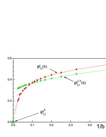
Figure 3: Results obtained in this work for the contact critical exponent $\varphi_{32}$ for the two-polymer system, when the first polymer is a floating 3D SG chain, while the other is a 2D SG adsorbed chain. The red triangles represent the MCRG values, while green triangles correspond to the CA values calculated from (22). The green circle depicts the tree-dimensional Euclidean value $\varphi_{32}^{E}\approx 0$. The thin solid lines (red and green) represent a simple interpolation of data, while the red dotted lines show the two possible scenarios for the fractal-to-Euclidean behaviour of $\varphi_{32}$, and serve as the guides to the eye. The error bars, for the MCRG data, are not depicted in the figure, since in all cases they lie within of the corresponding symbols (red triangles).

Table 2: Numerical values for the contact critical exponents $\varphi_{32}$, $\varphi_{33}$ and $\varphi_{22}$ evaluated from the proposed phenomenological formulae (based on the CA arguments) (22)–(24). The values for $\nu_{3}$ and $\nu_{2}$ have been calculated through the MCRG simulations performed in [21] and [24], respectively.

$b\$ $\nu_{3}$ $\nu_{2}$ $\varphi_{32}^{{}_{CA}}$ $\varphi_{33}^{{}_{CA}}$ $\varphi_{22}^{{}_{CA}}$ 2 0.6742 0.7985 0.4959 0.6516 0.7344 3 0.6543 0.7937 0.4530 0.6287 0.7055 4 0.6414 0.7882 0.4277 0.6140 0.6908 5 0.6315 0.7840 0.4105 0.6050 0.6808 6 0.6239 0.7801 0.3981 0.5984 0.6745 7 0.6169 0.7773 0.3890 0.5953 0.6689 8 0.6130 0.7742 0.3805 0.5887 0.6658 9 0.6087 0.7722 0.3738 0.5855 0.6622 10 0.6048 0.7698 0.3690 0.5833 0.6603 12 0.5987 0.7659 0.3608 0.5792 0.6571 15 0.5933 0.7620 0.3497 0.5711 0.6529 17 0.5899 0.7590 0.3455 0.5683 0.6523 20 0.5869 0.7560 0.3384 0.5621 0.6506 25 0.5817 0.7516 0.3317 0.5577 0.6495 30 0.5795 0.7481 0.3249 0.5502 0.6491 35 0.5759 0.7457 0.3212 0.5490 0.6480 40 0.5755 0.7434 0.3158 0.5416 0.6479

In figure 3, we have also presented the numerical values for $\varphi_{32}$, that follow from the CA argument predictions adopted for the studied model. Namely, the CA argument claims that a codimension $d-d_{ip}$ of intersection points is a sum of codimensions $d-d_{1}$ and $d-d_{2}$ of intersecting objects [16, 26]. Here, $d$ is a dimension of embedded space, $d_{ip}$ dimension of intersection points, and, $d_{1}$ and $d_{2}$ dimensions of intersecting objects. In the studied problem the embedded space is a 3D SG fractal of fractal dimension $d_{f}^{3D}$, while the intersecting objects are linear polymers with the fractal dimensions $d_{1}=1/\nu_{3}$ and $d_{2}=1/\nu_{2}$, whereupon follows

$$d_{ip}=\left({1\over\nu_{3}}+{1\over\nu_{2}}\right)-d_{f}^{3D}\>.$$ (20)

On the other hand, the total number of intersection points behaves according to the power law

$$M_{32}\sim\langle R_{N}\rangle^{d_{ip}}\sim N^{\nu_{3}d_{ip}}\>,$$ (21)

where $\langle R_{N}\rangle\sim N^{\nu_{3}}$ is the mean end-to-end distance of the longer polymer chain. From the latter scaling form, we find the following phenomenological formula for the contact critical exponent

$$\varphi_{32}^{{}_{CA}}=\left(1+{\nu_{3}\over\nu_{2}}\right)-\nu_{3}d_{f}^{3D}\>,$$ (22)

whose numerical values, evaluated from the attainable values for $\nu_{3}$ and $\nu_{2}$ on SG fractals, are listed in table 2. Comparing the values for $\varphi_{32}$ predicted by the obtained CA formula with our convincing set of MCRG data (see figure 3), we can perceive that in the first part of the examined region ($2\leq b\leq 40$), the CA formula displays satisfactory agreement with the corresponding MCRG values, and, for example, for $b=10$ fractal the two data (CA and MCRG) have almost identical numerical values. For $b<10$, the CA formula gives some smaller values for $\varphi_{32}$ than the MCRG method (at most 9%, for $b=2$), while for $b>10$, the CA predicted values get to be larger than the corresponding MCRG findings, and, when $b$ increases, a departure of the two sets of data becomes unambiguous (for $b=40$, the deviation is 57%). Anyway, from both the MCRG method and the CA formula (22), follow that $\varphi_{32}$, in the studied region, is a monotonically decreasing function of $b$.

Besides of $\varphi_{32}$, we may define the critical exponent $\varphi_{33}$ which describes the number of polymer-polymer contacts, when both polymers are floating chains in the 3D SG fractal container (that is, when both polymers are of the type $P_{3}$), and $\varphi_{22}$ when both polymers are adsorbed by 2D SG surface (both of the type $P_{2}$). For these exponents the CA arguments give

$$\varphi_{33}^{{}_{CA}}=2-\nu_{3}d_{f}^{3D}\>,$$ (23)

$$\varphi_{22}^{{}_{CA}}=2-\nu_{2}d_{f}^{2D}\>.$$ (24)

A simple comparison of the data, from table 2, reveals that the following relationship holds

$$\varphi_{32}<\varphi_{33}<\varphi_{22}\>,$$ (25)

for each particular $b$, in the range $2\leq b\leq 40$. The first inequality means that the number of polymer contacts increases when both polymers being situated in the bulk of 3D SG fractal, because of growing fractal dimension of a polymer chain when it makes a transition from the 2D SG surface to the bulk of 3D SG fractal ($d_{f}^{P_{3}}=1/\nu_{3}>d_{f}^{P_{2}}=1/\nu_{2}$). On the other hand, in the case when both polymers are adsorbed (situated on 2D SG fractal), the fractal dimension of the embedded space decreases $d_{f}^{2D}<d_{f}^{3D}$, and a chance for two polymers to make a contact increases, implying the second inequality in (25).

The relation between $\varphi_{32}$ and $\varphi_{22}$, can be tested on the reliable sets of MCRG values for $\varphi_{32}$ (calculated in this work) and $\varphi_{22}$ (calculated previously [18] in the range $2\leq b\leq 100$). The values for $\varphi_{22}$, being always larger than the corresponding CA values proposed by (24), display a monotonic decreasing from $\varphi_{22}(b=2)=0.7493$ up to $\varphi_{22}(b=100)=0.6735$ [18]. Their comparison with $\varphi_{32}$ (from table 1) shows that the relation $\varphi_{32}<\varphi_{22}$ is always satisfied. The relations between $\varphi_{33}$ and the other two contact critical exponents ($\varphi_{32}$ and $\varphi_{22}$) can be numerically proved only for $b=2$ fractal, where the RG value is known $\varphi_{33}(b=2)=0.6635$ [20], and from which the CA value 0.6516 deviates only 1.8%. To complete the inspection of relation (25) and test CA formula (23) for larger $b$, one needs to calculate $\varphi_{33}$ values for $b>2$, which appears to be much complicated task than the calculation of $\varphi_{32}$, and may be a topic for a future study.

Finally, we discuss the possible behaviour of the contact critical exponents in the fractal-to-Euclidean crossover region, that is, in the limit $b\to\infty$ ($d_{f}^{3D}\to 3$, $d_{f}^{2D}\to 2$). For a SAW situated in Euclidean spaces, the end-to-end distance critical exponent in $d=2$ takes the exact value $\nu_{2}^{E}=3/4$ [27], that was numerically confirmed [28] for the triangular lattice (to which the 2D SG fractals approach, when $b\to\infty$), whereas in $d=3$, at present, the most accurate evaluates are $\nu_{3}^{E}=0.5874\pm 0.0002$ [29] and $\nu_{3}^{E}=0.58765\pm 0.00020$ [30]. Consequently, from the formulas (22)–(24), we compute the Euclidean values: $\varphi_{32}^{E}\approx 0$, $\varphi_{33}^{E}\approx 1/5$ and $\varphi_{22}^{E}=1/2$. In the case of 2D SG fractals (when both polymers are of the type $P_{2}$), using the finite-size scaling arguments it was argued [20], that in the limit $b\to\infty$, the asymptotic behaviour of $\varphi_{22}$ is described by the relation $\varphi_{22}\simeq 2-\nu_{2}d_{f}^{2D}$, which coincides with the CA formula (24). Knowing, from the finite-size scaling analysis [31], that $\nu_{2}$ for very large $b$ goes, from below, to the Euclidean value $3/4$, from the latter asymptotic relation follows that $\varphi_{22}$ approaches, from above, the Euclidean value $\varphi_{22}^{E}=1/2$, when $b\to\infty$.

As regards the obtained MCRG results for $\varphi_{32}$, it is hard to say what happens beyond $b=40$, and specially, to establish whether the critical exponent $\varphi_{32}$, in the limit $b\to\infty$, goes to the zero Euclidean value, or some non-Euclidean value (see figure 3). To answer this question properly, another method may be needed, for instance, the finite-size scaling approach that has been applied in the case of 2D SG fractals [20, 31]. Here, we can only discuss possible predictions, about the limiting value for $\varphi_{32}$, that follow from the corresponding CA formula, for which we need to know the asymptotic behaviour of $\nu_{3}$. Unfortunately, up today, the behaviour of $\nu_{3}$, in the fractal-to-Euclidean crossover region $b\to\infty$, exists as an unsolved problem. At this moment, we may say that if $\nu_{3}\to\nu_{3}^{E}$ (which means, see data from table 2, that $\nu_{3}$ is a non-monotonic function of $b$), then (22) gives $\varphi_{32}\to\varphi_{32}^{E}\approx 0$. On the contrary, if $\nu_{3}$ tends to some non-Euclidean value less than $\nu_{3}^{E}$, then $\varphi_{32}$ will go to some value larger than the Euclidean value $\varphi_{32}^{E}$. The possibility that $\nu_{3}$, for $b\to\infty$, tends to some value larger than $\nu_{3}^{E}$ should imply a negative value of $\varphi_{32}$ (and consequently, in this case, we cannot exclude a situation in which the studied transition turns into first order, with increasing $b$). Similar conclusions may be deduced about the limiting value for the contact critical exponent $\varphi_{33}$. Particulary, from (23) follows: if $\nu_{3}\to\nu_{3}^{E}$ then $\varphi_{33}\to\varphi_{33}^{E}\approx 1/5$, or, if $\nu_{3}$ approaches the non-Euclidean value, then $\varphi_{33}$ also approaches a non-Euclidean value. From the exposed analysis we may infer that the behaviour of the contact critical exponents, in the fractal-to-Euclidean crossover region, is closely related to the corresponding behaviour of the end-to-end distance critical exponents.

4 Summary

In this paper we have studied the two interacting linear polymer chains, modelled by two mutually crossing SAWs, situated on fractal structures represented by the three-dimensional (3D) Sierpinski gasket (SG) family of fractals. We take on that the first polymer ($P_{3}$) is a floating chain in the bulk of 3D SG fractal, while the second polymer chain ($P_{2}$) is adsorbed onto one of the four boundaries of the 3D SG fractal, which appears to be 2D SG fractal. Specifically, we have calculated the contact critical exponent $\varphi_{32}$, associated with the number of monomer-monomer contacts between polymers $P_{3}$ and $P_{2}$.

By applying the renormalization group (RG) method, we have calculated the exact value of the critical exponent $\varphi_{32}$, for the first member $b=2$ of 3D SG fractal family. The specific accomplishment in the course of this work is the calculation of a long sequence of values of $\varphi_{32}$, for $2\leq b\leq 40$, obtained by applying the Monte Carlo renormalization group (MCRG) method. Our results demonstrate that $\varphi_{32}$, for the studied values of $b$, monotonically decrease with $b$, and, in analogy with the behaviour of $\varphi_{22}$ (that governs the number of contacts between two adsorbed polymers) it seems that for $b>40$ the critical exponent $\varphi_{32}$ continues decreasing, and in the limit $b\to\infty$ tends to the Euclidean value $\varphi_{32}^{E}\approx 0$. Finally, using the codimension additivity (CA) arguments we have proposed the phenomenological formulae for the considered contact critical exponents, and we have tested their predictions on the obtained sets of data. We find that, for fractals labelled by smaller values of $b$, the CA proposals give satisfactory agreement with existing convincing results.

On the exposed grounds of the presented investigation we may conclude that the set of obtained results of the studied problem has been significantly extended. We have demonstrated that the statistics of two crosslinked polymer chains on the family of 3D SG fractals can be rewardingly studied by the MCRG method. In particular, the MCRG study of the contact critical exponents revealed their interesting behaviour as the functions of fractal scaling parameter $b$, making a step forward to prescribe the behaviour of SAW critical exponents in the fractal-to-Euclidean crossover region. As a further investigation one may attempt to extend our study for calculating the contact critical exponent $\varphi_{33}$, when both polymers are floating chains in the bulk of 3D SG fractal. In addition, to make the studied model more realistic (but more difficult to study), it can be supplemented by additional interactions. For instance, one can introduce the interactions between the bulk floating chain and the sites of adsorbing surface (to promote the adsorbed phase of floating chain), as well as the intra-chain interactions (to promote a collapsing phase of the bulk floating chain), and then, in the space of interaction parameters the phase diagram can be investigated, together with new contact critical exponents at appropriate phase transition fixed points.

References

References

- [1] Vanderzande C, 1998 Lattice Models of Polymers (Canbridge: Cambrige University Press)
- [2] Brak R, Essam J W and Owczarek A L, Exact solution of directed non-intersecting walks interacting with one or two boundaries, 1999 J. Phys. A: Math. Gen. 32 2921
- [3] Freed K F, New lattice model for interacting, avoiding polymers with controlled length distribution, 1985 J. Phys. A: Math. Gen. 18 871
- [4] Sariban A and Binder K, Critical properties of the Flory-Huggins lattice model of polymer mixtures, 1987 J. Chem. Phys. 86 5859
- [5] Pelissetto A and Vicari E, Corrections to scaling in multicomponent polymer solutions, 2006 Phys. Rev. E 73 051802.
- [6] Haddad T A S, Andrade R F S and Salinas S R, Critical properties of an aperiodic model for interacting polymers, 2004 J. Phys. A: Math. Gen. 37 1499
- [7] Benhamou M, Derouiche A and Bettachy A, Microphase separation of crosslinked polymer blends in solution, 1997 J. Chem. Phys. 106 2513
- [8] Müller S and Schäfer L, On the number of intersections of self-repelling polymer chains, 1998 Eur. Phys. J. B 2 351
- [9] Westfahl H and Schmalian J, Correlated disorder in random block copolymers, 2005 Phys. Rev. E 72 011806.
- [10] Orlandini E, Seno F and Stella A L, Adsorption-like Collapse of diblock Copolymers, 2000 Phys. Rev. Lett. 84 294
- [11] Baiesi M, Carlon E, Orlandini E and Stella A L, Zipping and collapse of diblock copolymers, 2001 Phys. Rev. E 63 041801
- [12] Marenduzzo D, Bhattacharjee S M, Maritan A, Orlandini E and Seno F, Dynamical scaling of DNA unzipping transition, 2002 Phys. Rev. Lett. 88 028102
- [13] Kapri R, Bhattacharjee S M and Seno F, Complete Phase Diagram of DNA Unzipping: Eye, Y-fork and triple point, 2004 Phys. Rev. Lett. 93 248102
- [14] Kumar S, Giri D and Bhattacharjee S M, Force induced triple point for interacting polymers, 2005 Phys. Rev. E 71 051804
- [15] Kumar S and Singh Y, Critical behaviour of two interacting linear polymer chains: exact results for a state of interpenetration of chains on a fractal lattice, 1993 J. Phys. A: Math. Gen. 26 L987
- [16] Leoni P, Vanderzande C and Vandeurzen J, Zipping transition in a model of two crosslinked polymers, 2001 J. Phys. A: Math. Gen. 34 9777
- [17] De’Bell K and Lookman T, Surface phase transitions in polymer systems, 1993 Rev. Mod. Phys. 65 87
- [18] Živić I and Milošević S, Monte Carlo renormalization group study of crosslinked polymer chains on fractals, 1998 J. Phys. A: Math. Gen. 31 1372
- [19] Miljković V, Živić I and Milošević S, On the number of contacts of two polymer chains situated on fractal structures, 2004 Eur. Phys. J. B 40 55
- [20] Kumar S and Singh Y, Critical behaviour of two interacting linear polymer chains in a good solvent, 1997 J. Stat. Phys. 89 981
- [21] Elezović-Hadžić S, Živić I and Milošević S, Exact and Monte Carlo study of adsorption of a self-interacting polymer chain for a family of three-dimensional fractals, 2003 J. Phys. A: Math. Gen. 36 1213
- [22] Kumar S and Singh Y, Adsorption and collapse transitions of a linear polymer chain interacting with a surface adsorbed polymer chain, 2001 Physica A 293 345
- [23] Elezović-Hadžić S, Knežević M and Milošević S, Critical exponents of the self-avoiding walks on a family of finitely ramified fractals, 1987 J. Phys. A: Math. Gen. 20 1215
- [24] Živić I and Milošević S, Self-avoiding walks on fractals studied by the Monte Carlo renormalization group, 1991 J. Phys. A: Math. Gen. 24 L833
- [25] Dhar D, Self-avoiding random walks: Some exactly soluble cases, 1978 J. Math. Phys. 19 5
- [26] Mandelbrot B B, 1982 The Fractal Geometry of Nature (San Francisco: Freeman)
- [27] Nienhuis B, Exact critical point and critical exponents of O() models in two dimensions, 1982 Phys. Rev. Lett. 49 1062
- [28] Jensen I, Self-avoiding walks and polygons on the triangular lattice, 2004 J. Stat. Mech. P10008
- [29] Prellberg T, Scaling of self-avoiding walks and self-avoiding trails in three dimensions, 2001 J. Phys. A: Math. Gen. 34 L599
- [30] Hsu H P, Nadler W and Grassberger P, Scaling of Star Polymers with 1–80 Arms, 2004 Macromolecules 37 4658
- [31] Dhar D, Critical exponents of self-avoiding walks on fractals with dimension 2-, 1988 J. Physique 49 397