Heat production and energy balance in nanoengines driven by time-dependent fields.

Abstract

We present a formalism to study the heat transport and the power developed by the local driving fields on a quantum system coupled to macroscopic reservoirs. We show that, quite generally, two important mechanisms can take place: (i) directed heat transport between reservoirs induced by the ac potentials and (ii) at slow driving, two oscillating out of phase forces perform work against each other, while the energy dissipated into the reservoirs is negligible.

The understanding of the heat transport at the microscopic realm has attracted the attention of theoreticians for several years now. Several studies investigate this issue in the framework of one-dimensional lattice models of interacting classical oscillators. fer ; cam ; gen ; giar ; pere Nowadays, the technological trend towards the fabrication of nanosize electronic devices, is boosting the theoretical interest in quantum transport in a variety of setups and materials. Recently, there have been efforts to address the related problems of energy transport and heat dissipation in these small-size systems. AEGS01 ; mobu ; wan ; linkeheat ; nitzan ; bee ; rey

Electronic quantum transport through mesoscopic systems has been traditionally analyzed as a response to dc-voltages. There are, however, alternative possibilities to induce net transport by using time-dependent fields as the generating source. Interesting examples of this kind have been recently realized experimentally. pumpex ; saw An important characteristic of these systems is that directed motion is realized by pure ac forces thanks to the convenient breaking of relevant symmetries. Brouwer98 ; flach ; lilipr

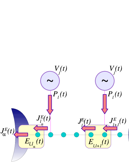
Figure 1: (Color online) Sketch of the device. The sites of the chain described by $H^{sys}(t)$ are represented by small circles. The local harmonically time-dependent fields $V_{j}(t)$ develop a power $\overline{P}_{j}$. The right box encloses a unit of chain described by $H^{l,l+1}(t)$ where energy conservation is considered, while the left one corresponds to a unit described by $H^{(cont)}$. The arrows indicate the dc energy currents $\overline{J}^{E}_{l}$ flowing into a bond $(l,l+1)$ of the system, $\overline{J}^{E}_{l_{\alpha}}$ entering the contacts and $\overline{J}^{E}_{\alpha}$ entering the reservoirs.

Energy transport in stationary conditions is achieved as a response to temperature and/or chemical potential gradients. The application of time dependent fields can induce net particle transport between reservoirs at the same chemical potentials, while it brings about by itself heating of the sample. Then, it is possible that ac forces can also generate directed heat transport between those reservoirs even if they are at the same temperatures. If so: What determines the direction of that heat flow? In general: What is the detailed energy balance for such a system? Is it possible to transport part of this energy to develop work? The theoretical study of the underlying physical processes demands a full quantum-mechanical treatment of the problem to evaluate the heat currents through the different parts of the device, as well as the calculation of the powers developed by the external fields. The aim of this work is to present a theoretical approach based in non-equilibrium Green’s function that will allow us to address details of the energy balance in the framework of an exactly solvable model of an electronic quantum pump.lilip

The device can be described in terms of a Hamiltonian with three pieces representing the electronic driven system, the contact to the reservoirs and the reservoirs: $H(t)=H^{sys}(t)+H^{cont}+H^{res}$. For simplicity, we consider a two terminal setup with left ($L$) and right ($R$) reservoirs, and a $N$-site one-dimensional lattice model for the driven system. We assume that the latter has an energy profile $\varepsilon^{0}_{l}$ and nearest neighbor hopping elements $w_{l}$. At $M$ lattice positions, ac potentials of the form $V_{j}(t)=V_{j}\cos(\Omega_{0}t+\varphi_{j})$ are locally applied. This system Hamiltonian can, thus, be expressed as $H^{sys}(t)=\sum_{l=1}^{N-1}H^{(l,l+1)}(t)$, being

$$H^{(l,l+1)}(t) = \varepsilon_{l}(t)c^{\dagger}_{l}c_{l}+\varepsilon_{l+1}(t)c^{\dagger}_{l+1}c_{l+1}$$ (1)

$$-w_{l}\Big{(}c^{\dagger}_{l}c_{l+1}+c^{\dagger}_{l+1}c_{l}\Big{)},$$

with $\varepsilon_{l}(t)=\zeta_{l}\Big{(}\varepsilon^{0}_{l}+\sum_{j=1}^{M}\delta_{l,l_{j}}V_{j}(t)\Big{)}$, being $\zeta_{l}=1/2$ for $1<l<N$ and $\zeta_{l_{\alpha}}=1$, for the sites that intervene in the connection to the reservoirs $l_{\alpha}\equiv 1,N$. The contacts are represented by hopping terms between the reservoirs and the latter positions: $H^{cont}=\sum_{\alpha,k_{\alpha}}w_{\alpha}(c^{\dagger}_{k_{\alpha}}c_{l_{\alpha}}+H.c.)$. The reservoirs are described by free-electron models: $H^{res}=\sum_{k_{\alpha}}\varepsilon_{k_{\alpha}}c^{\dagger}_{k_{\alpha}}c_{k_{\alpha}}$, which are assumed to remain at equilibrium with well defined chemical potentials $\mu_{\alpha}$ and temperatures $T_{\alpha}$, even after being connected to the driven structure.

In order to define currents of energy, we can follow the quantum mechanical counterpart of the procedure carried out in Refs. cam ; pere for a classical model. We formulate the equation for the conservation of the energy $E_{l,l+1}(t)=\langle H^{(l,l+1)}(t)\rangle$ stored in a bond $(l,l+1)$. The variation in time of this mean value is calculated by recourse to Ehrenfest’s theorem which casts:

$$\frac{dE_{l,l+1}(t)}{dt}=J^{E}_{l+1}(t)-J^{E}_{l}(t)+\frac{1}{2}\Big{(}P_{l}(t)+P_{l+1}(t)\Big{)},$$ (2)

$$\frac{dE_{\alpha,l_{\alpha}}(t)}{dt}=J^{E}_{l_{\alpha}}(t)-J^{E}_{\alpha}(t)+\frac{1}{2}P_{l_{\alpha}}(t),$$ (3)

where the first equation corresponds to bonds of the system without sites in contact to reservoirs (i.e. $1<l<N-1$), as the one enclosed by the right box of Fig. 1, while the second one corresponds to the left bond that establishes the contact between system and reservoir (see left box of Fig. 1). The first two terms of (2) represent a discretized version of the divergence of the energy current flowing through the bond, while the last two terms represent the power developed by the external forces and are equal to $\langle\partial H^{(l,l+1)}(t)/\partial t\rangle$. In Eq. (3), the first current represents the flow of energy towards the system, the second one is the flow of energy entering the reservoir, and the third one, the power developed by the external forces.

Denoting $\rho_{j,j^{\prime}}(t)=\langle c^{\dagger}_{j^{\prime}}(t)c_{j}(t)\rangle$, the explicit expressions for the different energy currents read:

$$J^{E}_{l}(t) = 2\mbox{Im}\Big{\{}\varepsilon_{l}(t)\Big{[}\rho_{l,l-1}(t)w_{l-1}-\rho_{l,l+1}(t)w_{l}\Big{]}$$

$$+w_{l-1}\rho_{l-1,l+1}(t)w_{l}\Big{\}},$$

$$J^{E}_{{\alpha}}(t) = -2\mbox{Im}\Big{\{}\sum_{k_{\alpha}}w_{\alpha}\rho_{l_{\alpha},k_{\alpha}}(t)\varepsilon_{k_{\alpha}}\Big{\}},$$ (5)

and a similar expression for $J^{E}_{l_{\alpha}}(t)$, while the power developed by the external forces is:

$${P}_{l}(t)=\sum_{j=1}^{M}\delta_{l,l_{j}}\frac{dV_{j}(t)}{dt}\rho_{l_{j},l_{j}}(t).$$ (6)

In order to analyze the energy balance we focus on the dc components of the energy currents and powers done by the external forces. The conservation of the energy (2) and (3) implies $\overline{dE_{l,l+1}(t)/dt}=0$ and $\overline{dE_{\alpha,l_{\alpha}}(t)/dt}=0$, which defines continuity equations for the dc energy currents $\overline{J}^{E}_{l}$, $\overline{J}^{E}_{\alpha}$ and powers $\overline{P}_{l}$, where $\overline{A}\equiv 1/\tau_{0}\int_{0}^{\tau_{0}}dtA(t)$, being $\tau_{0}=2\pi/\Omega_{0}$ the period of the oscillating time-dependent fields.

To evaluate the different energy currents and powers we employ the treatment based in Keldysh non-equilibrium Green’s functions of Ref. lilip , which has been useful to study charge transport in the kind of systems we are considering. The mean values of observables entering the corresponding expressions can be expressed in terms of lesser Green’s functions as follows $\rho_{j,j^{\prime}}(t)=-iG^{<}_{j,j^{\prime}}(t,t)$. The latter is evaluated from a Dyson equation, which for $j,j^{\prime}$ lying on the central system reads:

$$G^{<}_{l,l^{\prime}}(t,t) = \sum_{\alpha=L,R}\sum_{kk^{\prime}=-\infty}^{\infty}e^{-ik\Omega_{0}t}\int_{-\infty}^{\infty}\frac{d\omega}{2\pi}\Gamma^{<}_{\alpha}(\omega)$$ (7)

$$\times{\cal G}_{l,l_{\alpha}}(k+k^{\prime},\omega){\cal G}^{*}_{l^{\prime},l_{\alpha}}(k^{\prime},\omega),$$

being $\Gamma^{<}_{\alpha}(\omega)=if_{\alpha}(\omega)\Gamma_{\alpha}(\omega)$, where the Fermi function $f_{\alpha}(\omega)$ depends on $\mu_{\alpha}$ and $T_{\alpha}$, and $\Gamma_{\alpha}(\omega)=2\pi\sum_{k_{\alpha}}|\epsilon_{k_{\alpha}l_{\alpha}}|^{2}\delta(\omega-\varepsilon_{k_{\alpha}})$. The Green’s function ${\cal G}_{l,l^{\prime}}(k,\omega)$ is the $k$-th Fourier coefficient of the Fourier transform of the retarded Green’s function, which can be exactly evaluated with convenient methods. lilip The above expression (7) can be used in (Heat production and energy balance in nanoengines driven by time-dependent fields.) and (6) to evaluate $\overline{J}^{E}_{l}$ and $\overline{P}_{l_{j}}$. Using properties of the Green’s function lilimich the dc component of the energy current flowing into the reservoir reads:

$$\overline{J}^{E}_{\alpha} = \sum_{\beta=L,R}\sum_{k=-\infty}^{\infty}\int\frac{d\omega}{2\pi}(\omega+k\Omega_{0})\Gamma_{\alpha}(\omega+k\Omega_{0})\Gamma_{\beta}(\omega)$$ (8)

$$\times|{\cal G}_{l_{\alpha},l_{\beta}}(k,\omega)|^{2}\Big{[}f_{\beta}(\omega)-f_{\alpha}(\omega+k\Omega_{0})\Big{]}.$$

We are interested in the case of reservoirs at the same chemical potentials $\mu_{\alpha}=\mu,\forall\alpha$. Following the same line as in stationary transport at linear response,bee we define the dc-heat current as $\overline{J}_{\gamma}^{Q}=\overline{J}_{\gamma}^{E}-\mu\overline{J}_{\gamma}^{C}$, the latter term being the convective flow which depends on the dc-charge current $\overline{J}_{\gamma}^{C}$.note As this current is conserved, $\overline{J}_{\gamma}^{Q}$ obeys the same continuity equation satisfied by $\overline{J}_{\gamma}^{E}$.

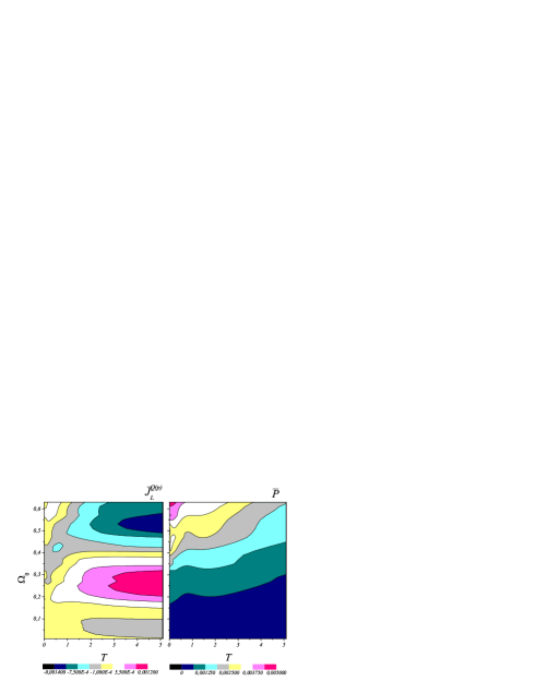
Figure 2: (Color online) Pumped heat current (left) and total power $P=\overline{P}_{1}+\overline{P}_{2}$ developed by the forces (right) as functions of temperature and the pumping frequency. Parameters are $N=22$, $E=1$, $V=0.2$, $T=0$, $\varphi=\pi/2$ and $\mu=-1.5$.

We now use the above theoretical framework to analyze two generic mechanisms that can take place in quantum pumps. The first one concerns the possibility of achieving directed heat transport between reservoirs. To this end, notice, that the dc-heat current along the lead $\alpha$ can be splitted as the addition of a generated and a pumped contribution: $\overline{J}_{\alpha}^{Q}=\overline{J}_{\alpha}^{Q(g)}+\overline{J}_{\alpha}^{Q(p)}$, where the pumped component reads explicitly:

$$\overline{J}^{Q(p)}_{\alpha} = \int\frac{d\omega}{2\pi}(\omega-\mu)\Big{\{}2\Gamma^{<}_{\alpha}(\omega)\mbox{Im}[{\cal G}_{l_{\alpha},l_{\alpha}}(0,\omega)]+$$

$$\sum_{\beta=L,R}\sum_{k=-\infty}^{\infty}\Gamma_{\alpha}(\omega+k\Omega_{0})\Gamma^{<}_{\beta}(\omega)|{\cal G}_{l_{\alpha},l_{\beta}}(k,\omega)|^{2}\Big{\}}.$$

This component can be proved to satisfy $\sum_{\alpha=L,R}\overline{J}^{Q(p)}_{\alpha}=0$, meaning that heat can be extracted from a given reservoir and injected into the other one. From the continuity equation for the dc heat current, it follows that $\sum_{j=1}^{M}\overline{P}_{l_{j}}=\sum_{\alpha=L,R}\overline{J}^{Q(g)}_{\alpha}$, indicating that the $\overline{J}^{Q(g)}_{\alpha}$ contribution accounts for the heat generated by the external forces, which is dissipated into the reservoirs.

An example of the behavior of these two different contributions to the heat flows at the reservoirs is shown in Fig. 2 for a two barrier setup in contact to reservoirs at the same temperature $T_{L}=T_{R}=T$. We consider $\varepsilon^{0}_{l_{j}}=E$, $l_{j}=2,N-1$ and $\varepsilon^{0}_{l_{j}}=0,l\neq l_{j}$, with two oscillating potentials with the same amplitude $V$ and a phase-lag $\varphi_{1}=\varphi$,$\varphi_{2}=0$ applied at the barriers. Under such conditions a dc charge current $\overline{J}^{C}$ is induced which behaves like $\overline{J}^{C}\propto V^{2}\sin(\varphi)$ at small $V$. Brouwer98 The pumped component of the heat current, shown in the left panel of Fig. 2, flows outwards in a reservoir and inwards in the other one. It exhibits a complex structure of maxima, minima and sign inversions as a function of $\Omega_{0}$. The details of these features are model-dependent. They are consequence of the electronic propagation through a structure with discrete energy levels and quantum interference that takes place when the pumping frequency $\Omega_{0}$ is resonant with the energy difference between these levels. mobu The generated heat currents at the different leads $\overline{J}^{Q(g)}_{L,R}$, also display a complex landscape in the $T,\Omega_{0}$ plane. Their sum is, however, always positive and equals the total developed power $\overline{P}=\overline{P}_{1}+\overline{P}_{2}$, which is a monotonous increasing function of $\Omega_{0}$ and decreases with $T$ as shown in the right panel of Fig. 2.

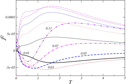
Figure 3: (Color online) Total heat current as functions of $T$ for different pumping frequencies. Thin and thick lines correspond to $\overline{J}^{Q}_{L}$ and $\overline{J}^{Q}_{R}$, respectively. Parameters are as in Fig. 2. The values of $\Omega_{0}$ are indicated in the plots.

At $T=0$ dissipation dominates and masks the heat pumping effect. For our example, the total heat currents $\overline{J}_{L}^{Q},\overline{J}_{R}^{Q}$ as functions of $T$ are plotted in Fig. 3. There it is seen that the sign of both currents is positive at $T=0$, which indicates that the flow goes from the central system towards the reservoirs. Such a behavior is the one expected from considerations based on general thermodynamics since, at $T=0$ there is no heat at the reservoirs amenable to be transported. However, the results of Fig. 3 show that at finite $T$ a regime exists for low pumping frequencies $\Omega_{0}$ where heat pumping takes place. In fact, the signs of the heat currents are different, indicating that they leave one of the reservoirs and enter the other one. For higher $\Omega_{0}$ dissipation is again dominant and heat flows always from the central system into the two reservoirs.

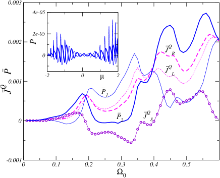
Figure 4: (Color online) Main Panel: Heat currents $\overline{J}^{Q}_{L},\overline{J}^{Q}_{R}$ (dashed thin and thick lines) and $\overline{J}^{Q}_{S}$ (circles) along the left and right leads and the central system, respectively for$\mu=-1.5$. Powers developed by the external fields $\overline{P}_{1},\overline{P}_{2}$ (thin and thick solid lines). Inset: $\overline{P}_{1},\overline{P}_{2}$ as function of $\mu$ for $\Omega_{0}=0.01$. Parameters are as in Fig. 2.

The second remarkable mechanism we would like to analyze is the possibility of extracting work from the system. This issue can be addressed on the basis of a perturbative solution of the Dyson equation which allows for the evaluation of $\overline{P}_{l_{j}}$ at the lowest order in $V_{j}$.lilip ; lilipr It casts:

$$\overline{P}_{l_{j}}\sim\sum_{i=1}^{M}\Big{[}\lambda^{(1)}_{ji}\cos(\varphi_{j}-\varphi_{i})+\lambda^{(2)}_{ji}\sin(\varphi_{j}-\varphi_{i})\Big{]},$$ (10)

where the coefficients are

$$\lambda^{(1)}_{ji} = \Omega_{0}\frac{V_{i}V_{j}}{2}\int_{-\infty}^{+\infty}\frac{d\omega}{2\pi}\mbox{Im}\Big{\{}\gamma_{ji}(\omega)\gamma^{-}_{ji}(\omega)\Big{\}},$$

$$\lambda^{(2)}_{ji} = \Omega_{0}\frac{V_{i}V_{j}}{2}\int_{-\infty}^{+\infty}\frac{d\omega}{2\pi}\mbox{Re}\Big{\{}\gamma_{ji}(\omega)\gamma^{+}_{ji}(\omega)\Big{\}},$$

with $\gamma_{ji}(\omega)=\sum_{\alpha=L,R}\Gamma^{<}_{\alpha}(\omega)[G^{0}_{l_{j},l_{\alpha}}(\omega)]^{*}G^{0}_{l_{i},l_{\alpha}}(\omega)$ and $\gamma^{\pm}_{ji}(\omega)=\Big{[}G^{0}_{l_{j},l_{i}}(\omega+\Omega_{0})\pm G^{0}_{l_{j},l_{i}}(\omega-\Omega_{0})\Big{]}$, being $G^{0}_{l,l^{\prime}}(\omega)$ the equilibrium retarded Green’s function of the system in contact to the reservoirs but without the time-dependent fields. In the low frequency limit, $\lambda^{(1)}_{ij}\propto\Omega_{0}^{2}$ while $\lambda^{(2)}_{ij}\propto\Omega_{0}$ . Thus, this solution indicates that quantum coherence in the wave function propagation along the structure, which rules the behavior of the charge current, also plays a role in the way in which energy is provided and exchanged. In particular, for more than one oscillating fields, the terms $\propto\lambda^{(2)}_{ij}$ dominate at low enough $\Omega_{0}$. Since these terms can be positive for some fields and negative for other ones, this enables a scenario where the total energy $\overline{P}=\sum_{j=1}^{M}\overline{P}_{j}$ is dissipated to the reservoirs at a ratio $\propto\Omega_{0}^{2}$, while a larger amount of energy $\propto\Omega_{0}$ is exchanged between the different pumping centers. Such an effect is, in fact, observed for some parameters in the example of the two-barrier setup. Results are shown in Fig. 4 for $T=0$ with $\varphi=\pi/2$. The dc powers are shown along with the dc heat currents $\overline{J}^{Q}_{L},\overline{J}^{Q}_{R}$ flowing to the reservoirs and the one flowing within the system between the two barriers $\overline{J}^{Q}_{S}$. The exchange of energy between the two fields is further highlighted in the inset where the two dc powers $\overline{P}_{1}$ and $\overline{P}_{2}$ as functions of $\mu$ are shown. It is also interesting to note that the direction of the heat flow between the two pumping centers, goes from the field doing the largest power towards the other one. Instead, in the reservoirs the heat currents are always positive, indicating that they flow inwards. These features are in line with the idea that the fields heat locally the sample inhomogeneously, then the heat current flows from the hottest to the coldest regions.

To conclude, we introduced a treatment based on the local conservation of the energy in order to investigate details of the energy transport in open quantum systems driven by time-dependent fields. We identified two interesting mechanisms like the possibility of achieving directed transport of heat between reservoirs at finite but identical temperature as well as extracting useful energy to make work against the external forces. We illustrated these effects in an exactly solvable model of an electronic quantum pump. Our results for reservoirs at $T=0$ also suggest that the direction of the heat flows seem to be ruled by an effective heat gradient induced by the application of the external driving.

We thank M. Büttiker for stimulating conversations. This work is supported by PICT 03-11609 and CONICET from Argentina, BFM2003-08532-C02-01 and the “Ramon y Cajal” program (LA) from MCEyC of Spain.

References

- (1) E. Fermi, J. Pasta and S. Ulam, Los Alamos Report No. LA-1940 (1955).
- (2) T. Prosen and D. K. Campbell, Phys. Rev. Lett. 84, 2857 (2000).
- (3) O. V. Gendelman and A.V. Sarvin, Phys. Rev. Lett 84, 2381 (2000); Phys. Rev. Lett 94, 219405 (2005).
- (4) C. Giardiná, et al, Phys. Rev. Lett 84, 2144 (2000).
- (5) E. Pereira and R. Falcao, Phys. Rev. Lett. 96, 100601 (2006).
- (6) J.E. Avron, A. Elgart, G.M. Graf, and L. Sadun, Phys. Rev. Lett. 87, 236601 (2001).
- (7) M. Moskalets and M. Büttiker Phys. Rev. B 66, 205320 (2002); ibid 70, 245305 (2004).
- (8) Y. Wei,et al, Phys. Rev. B 70, 045418 (2004).
- (9) T.E Humphrey, et al, Phys. Rev. Lett. 89, 116801 (2002); ibid 94, 096601 (2005).
- (10) D. Segal and A. Nitzan, Phys. Rev. Lett. 94, 034301 (2005).
- (11) H. van Houten, et al, Semicond. Sci. Technol. 7, B215 (1992).
- (12) M. Rey, M. Strass, S. Kohler, P. Hänggi and F. Sols, cond-mat/0610155.
- (13) L. J. Geerligs, et al, Phys. Rev. Lett. 64, 2691 (1990); M. Switkes, et al, Science 293, 1905 (1999); L. DiCarlo, C. M. Marcus and J. S. Harris, Phys. Rev. Lett. 91, 246804 (2003); S. K. Watson, et al, Phys. Rev. Lett. 91, 258301 (2003).
- (14) P. J. Leek, et al, Phys. Rev. Lett. 95, 256802 (2005).
- (15) P. W. Brouwer, Phys. Rev. B 58, R10135 (1998).
- (16) S. Flach, et al, Lett. 84, 2358 (2000).
- (17) L. Arrachea, Phys. Rev. B 72, 121306 (R) (2005) and Phys. Rev. B 72, 249904 (E) (2005).
- (18) L. Arrachea, Phys. Rev. B 72, 125349 (2005); ibid Phys Rev B. 72, (2006).
- (19) L. Arrachea and M. Moskalets, Phys Rev B. 72, (2006).
- (20) This procedure has also been followed in the context of time-periodic transport for the calculation of heat current flowing into the leads (see mobu, ; rey, ).