Entanglement-induced electron coherence in a mesoscopic ring
with two magnetic impurities

Abstract

We investigate the Aharonov-Bohm (AB) interference pattern in the electron transmission through a mesoscopic ring in which two identical non-interacting magnetic impurities are embedded. Adopting a quantum waveguide theory, we derive the exact transmission probability amplitudes and study the influence of maximally entangled states of the impurity spins on the electron transmittivity interference pattern. For suitable electron wave vectors, we show that the amplitude of AB oscillations in the absence of impurities is in fact not reduced within a wide range of the electron-impurity coupling constant when the maximally entangled singlet state is prepared. Such state is thus able to inhibit the usual electron decoherence due to scattering by magnetic impurities. We also show how this maximally entangled state of the impurity spins can be generated via electron scattering.

I Introduction

Phase coherence of electron motion is an important issue in mesoscopic physics. Indeed, preserving coherence of the conduction electrons is an essential requirement for the correct working of mesoscopic semiconductor devices relying on quantum mechanical phenomena datta ; hakenb . A well-known example of such systems is the Aharonov-Bohm (AB) ring washburn . Its features are due to the the phase difference acquired by the electrons passing on the upper and lower arms of the ring in the presence of a magnetic field. This gives rise to the well known interference pattern in the electron transmission as a function of the magnetic flux washburn ; xia . Scattering by magnetic impurities, and more in general by systems with an internal spin degree of freedom, is a well-known source of electron decoherence datta ; imrybook ; imry ; schulman . This follows from the uncertainty in the phase shift acquired by the scattered electron imry . Equivalently, decoherence can be viewed as due to the unavoidable scattering induced entanglement between the electron and impurity degrees of freedom imry ; schulman . The transmission properties of an AB ring with a single magnetic impurity inserted in one of the arms and with the electron and impurity spins interacting via a contact exchange coupling has been analyzed in joshi ; shi . When no spin-flip occurs – i.e. when the electron and impurity spins are initially aligned – the case of a static impurity is recovered mao and the amplitude of AB oscillations with no impurity is preserved in a wide range of values of the exchange coupling constant centered around zero joshi . However when spin-flip occurs, e.g. when the two spins are initially anti-aligned, the amplitude of AB oscillations is reduced. This is a signature of a loss of electron coherence which is larger for increasing strengths of the electron-impurity coupling constant joshi . In this paper we consider an AB ring with two identical spin-1/2 magnetic impurities, one embedded in each arm. Such system is not a mere academic extension of an AB ring with a single impurity but shows new phenomena. A new feature that appears in the presence of two spins is multiple scattering between the two impurities with simultaneous occurrence of spin-flip events. This leads to new cooperative phenomena. For instance, in the case of a 1D wire we have found that, under suitable resonance conditions, perfect transparency appears when the the two impurity spins are initially prepared in the singlet maximally entangled state ciccarello . In the present paper we will focus on the effects of entanglement between the impurity spins on the AB oscillations. Our main result is that, for suitable electron wave vectors, the amplitude of AB oscillations turns out to be in fact not reduced in a wide range of values of the coupling constant when the impurity spins are prepared in the maximally entangled singlet state $\left|\Psi^{-}\right\rangle$. This coherent transmission is due to an effective suppression of spin-flip events which occurs regardless of the electron spin state, at variance with the no spin-flip case which occurs when the electron and impurity spins are aligned joshi .

This paper is organized as follows. In Sec. II we introduce our system and illustrate the approach used to derive the exact transmission probability amplitudes. In Sec. III we investigate the AB oscillations for different spin states showing how a nearly coherent behavior is exhibited for the singlet state of the impurity spins. In Sec. IV we propose a scheme for generating this maximally entangled state via electron scattering. The detailed mathematical derivation of all the transmission probability amplitudes is provided in Appendix A.

II System and Approach

As illustrated in Fig. 1, our system consists of a conducting ring with equal arms. The circumference length is denoted by $L$. We assume the width of the structure to be narrow enough to let only the lowest electron subband to be accounted for. The effective mass of the electron is denoted by $m^{*}$. Two identical spin-1/2 impurities, labeled 1 and 2, are centered in the upper and lower arm, respectively (see Fig. 1). The left and right junctions of the ring are denoted by $C$ and $D$, respectively. A static magnetic field is applied perpendicularly to the ring plane across the internal region, excluding the wire and thus the two impurities (see gray shaded region in Fig. 1).

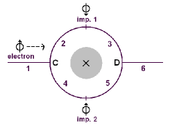
Figure 1: Mesoscopic ring with two magnetic impurities, labeled 1 and 2, inserted in the upper and lower arm, respectively. The left and right junctions are denoted with C and D, respectively. A static magnetic field is applied perpendicularly to the ring plane within the gray shaded region.

As in Refs. xia ; joshi ; shi ; mao ; amjphys , we adopt a quantum waveguide theory approach here properly generalized to take into account the presence of the two magnetic impurities. The local coordinate along the electron-current direction xia on the upper (lower) arm is denoted as $x_{1}$ ($x_{2}$), with $0\leq x_{i}\leq L/2$ ($i=1,2$). Both the above coordinates point to the junction $D$ with their origins being taken at $C$.

The Hamiltonian of the system can be written as

$$H=H_{0}+\sum_{i=1,2}H_{ei}$$ (1)

where $H_{0}$ is the Hamiltonian in the absence of impurities and $H_{ei}$ ($i=1,2$) describes the coupling between the electron spin $\sigma$ and the spin-1/2 of the $i$-th impurity $\mathbf{S}_{i}$. Denoting by $\mathbf{A}=\nabla\times\mathbf{B}$ the vector potential of the magnetic field $\mathbf{B}$ and by $\mathbf{p}=-i\hbar\nabla$ the electron momentum operator, $H_{0}$ has the well-known form

$$H_{0}=\frac{1}{2m^{*}}\,\left(\mathbf{p}+\frac{e}{c}\,\mathbf{A}\right)^{2}$$ (2)

As the vector potential is along the ring direction and has magnitude $A=\phi/L$, with $\phi$ standing for the magnetic flux through the ring section area, the effective representation $H_{0i}$ of (2) in the $i$-th arm is explicitly written as

$$H_{0i}=\frac{1}{2m^{*}}\,\left(\frac{\hbar}{i}\frac{d}{dx_{i}}+\xi\frac{e}{c}\,\frac{\phi}{L}\right)^{2}$$ (3)

with $\xi=-1$ ($+1$) for $i=1$ ($2$).

We model the electron-impurity spin-spin coupling as a contact exchange interaction according to

$$H_{ei}=-J\,\mbox{\boldmath$\sigma$}\cdot\mathbf{S}_{i}\,\delta(x_{i}-L/4)$$ (4)

where $J$ is the coupling constant, $x_{i}=L/4$ is the coordinate of the $i$-th impurity and where all the spin operators are in units of $\hbar$. At each electron-impurity scattering event no energy exchange takes place. However, the spin state of the two systems will, in general, change. In particular, if the electron and impurity spins are initially anti-aligned spin-flip may occur.

It is useful to rewrite the electron-impurity coupling Hamiltonian (4) in the form

$$H_{ei}=-\frac{J}{2}\left(\mathbf{S}_{ei}^{2}-\frac{3}{2}\right)\delta(x_{i}-L/4)\,\,\,\,\,\,\,\,\,(i=1,2)$$ (5)

where $\mathbf{S}_{ei}=\mbox{\boldmath$\sigma$}+\mathbf{S}_{i}$ is the total spin of the electron and the $i-$th impurity. Denoting by $\mathbf{S}=\mbox{\boldmath$\sigma$}+\mathbf{S}_{1}+\mathbf{S}_{2}$ the total spin operator, it turns out that $\mathbf{S}^{2}$ and $S_{z}$, with quantum numbers $s$ and $m_{s}=-s,...,s$, respectively, are constants of motion. It is thus convenient to use as spin space basis the states $\left|s_{e2};s,m\right\rangle$, common eigenstates of $\mathbf{S}_{e2}^{2}$ (quantum number $s_{e2}$), $\mathbf{S}^{2}$ and $S_{z}$ nota1 (from now on, the subscript $s$ in $m_{s}$ will be omitted). We denote by $t_{s_{e2}}^{(s^{\prime}_{e2},s)}$ the transmission probability amplitude that an electron injected from the left lead with wave vector $k$ and initial spin state $\left|s^{\prime}_{e2};s,m\right\rangle$ is transmitted in the right lead in the spin state $\left|s_{e2};s,m\right\rangle$. Note that, due to the form (5) of $H_{ei}$, the amplitudes $t_{s_{e2}}^{(s^{\prime}_{e2},s)}$ do not depend on $m$, as it will be made clearer in Appendix A. The amplitudes $t_{s_{e2}}^{(s^{\prime}_{e2},s)}$ can be exactly calculated by deriving the stationary states of the electron-two impurities system. Due to the conservation of $\mathbf{S}^{2}$ and $S_{z}$, their calculation can be carried on separately in each subspace of fixed $s$ and $m$. Note that, since $\mathbf{S}_{e1}^{2}$ (quantum number $s_{e1}$) and $\mathbf{S}_{e2}^{2}$ do not commute, $\mathbf{S}_{e2}^{2}$ is generally not conserved. Since we are coupling three spins 1/2, it turns out that the possible values of $s$ are 1/2 and 3/2. When $s=1/2$ the possible values of $s_{e2}$ are $s_{e2}=0,1$, while for $s=3/2$ we have $s_{e2}=1$ ($s_{e1}$ can assume the same values). For left-incoming electrons with wave vector $k$ there are eight stationary states and each of them can be expressed as an 8-dimensional column denoted as $\left|\Psi_{s^{\prime}_{e2};s,m}\right\rangle$, where $s^{\prime}_{e2}$ ($s=1/2\Rightarrow s^{\prime}_{e2}=0,1$; $s=3/2\Rightarrow s^{\prime}_{e2}=1$) is a labeling index which generally differs from $s_{e2}$. Note that since $s_{e1}=s_{e2}=1$ for $s=3/2$, in the subspace $s=3/2$, $\mathbf{S}_{e1}^{2}$ and $\mathbf{S}_{e2}^{2}$ effectively commute and thus no spin-flip can occur: the impurities behave as being static. This is not true for the subspace $s=1/2$, for which $s_{e1}$ and $s_{e2}$ can take values $0,1$. Therefore spin-flip in general takes place in the subspace $s=1/2$.

The knowledge of all coefficients $t_{s_{e2}}^{(s^{\prime}_{e2};s)}$, whose detailed calculation is carried on in Appendix A, completely describes the transmission properties of our system. Here we are mainly interested in calculating how an electron with a given wave vector $k$ and for some initial electron-impurities spin state $\left|\chi\right\rangle$ is transmitted through the device. Thus assuming to have the incident wave $\left|k\right\rangle\left|\chi\right\rangle$, with $\left|\chi\right\rangle$ being an arbitrary spin state, it is straightforward to see that $\left|k\right\rangle\left|\chi\right\rangle$ is the incoming part of the stationary state

$$\left|\Psi_{k,\chi}\right\rangle=\sum_{s_{e2}^{\prime},s,m}\langle s_{e2}^{\prime};s,m\left|\chi\right\rangle\left|\Psi_{s_{e2}^{\prime};s,m}\right\rangle$$ (6)

It follows that the transmitted part $\left|\Psi_{k,\chi}\right\rangle_{t}$ of (6) provides the transmitted state into which $\left|k\right\rangle\left|\chi\right\rangle$ evolves after its passage through the ring. To calculate $\left|\Psi_{k,\chi}\right\rangle_{t}$ we simply replace each stationary state $\left|\Psi_{s_{e2}^{\prime};s,m}\right\rangle$ in (6) with its transmitted part, express the latter in terms of amplitudes $t^{(s_{e2}^{\prime};s)}_{s_{e2}}$ and rearrange (6) as a linear expansion in the basis $\left|s_{e2};s,m\right\rangle$. This yields ciccarello

$$\left|\Psi_{k,\chi}\right\rangle_{t}=\left|k\right\rangle\sum_{s_{e2},s,m}\tau_{s_{e2},s,m}(\chi)\left|s_{e2},s,m\right\rangle\\$$ (7)

with

$$\tau_{s_{e2},s,m}(\chi)=\sum_{s_{e2}^{\prime}}t^{(s_{e2}^{\prime};s)}_{s_{e2}}\langle s_{e2}^{\prime};s,m\left|\chi\right\rangle$$ (8)

Coefficients (8) fully describe how an incoming wave $\left|k\right\rangle\left|\chi\right\rangle$ is transmitted through the mesoscopic ring. For instance, the total electron transmission coefficient $T$ can be calculated as

$$T=\sum_{s_{e2},s,m}|\tau_{s_{e2},s,m}(\chi)|^{2}$$ (9)

In Appendix A, we derive all the coefficients $t_{s_{e2}}^{(s^{\prime}_{e2},s)}$ through the calculation of the stationary states $\left|\Psi_{s^{\prime}_{e2};s,m}\right\rangle$.

III Aharonov-Bohm Oscillations

The coefficients $t_{s_{e2}}^{(s^{\prime}_{e2},s)}$ turn out to depend on the dimensionless parameters $kL$, $(2m^{*}/\hbar^{2})(J/k)$ and $\phi/\phi_{0}$ where $\phi_{0}=hc/e$ is the flux quantum. In Fig. 1 we plot the AB oscillations of electron transmission $T$ for $J/k=1,2,5$ (in unity of $2m^{*}/\hbar^{2}$) and $kL=1$ for an incoming electron in the state $\left|\uparrow\right\rangle$ and the impurity spins in the initial product states $\left|\uparrow\uparrow\right\rangle$ (a) and $\left|\uparrow\downarrow\right\rangle$ (b). In the first case, the amplitude of AB oscillations is negligibly reduced by an increase of $J/k$ in line with the no-spin flip scattering case for one magnetic impurity joshi . Indeed, when the state $\left|\uparrow\uparrow\right\rangle$ is prepared no spin-flip takes place since all the electron and impurity spins are aligned and the overall state $\left|\uparrow\right\rangle\left|\uparrow\uparrow\right\rangle$ belongs to the subspace $s=3/2$ where impurities behave as being static (see Sec. II). The behaviour of a ring with two static impurities mao is thus recovered. On the contrary, in the case $\left|\uparrow\downarrow\right\rangle$ (Fig. 2b) the amplitude of AB oscillations is rapidly reduced for increasing values of $J/k$ similarly to the spin-flip scattering case of Ref. joshi . Indeed, the initial overall spin state $\left|\uparrow\right\rangle\left|\uparrow\downarrow\right\rangle$ - which has non vanishing projection both on subspace $s=3/2$ and on the $s=1/2$ one - is generally changed by electron-impurities scattering into a linear combination of $\left|\uparrow\right\rangle\left|\uparrow\downarrow\right\rangle$, $\left|\uparrow\right\rangle\left|\downarrow\uparrow\right\rangle$ and $\left|\downarrow\right\rangle\left|\uparrow\uparrow\right\rangle$ indicating occurrence of spin-flip events. This induces loss of coherence as witnessed by the reduction of AB oscillations with $J/k$.

Figure 2: Total transmission coefficient $T$ versus magnetic flux $\phi/\phi_{0}$ for different values of $J/k$ and $kL=1$ for an incoming electron in the state $\left|\uparrow\right\rangle$ with the two impurities initially in the state $\left|\uparrow\uparrow\right\rangle$ (a) and $\left|\uparrow\downarrow\right\rangle$ (b). Solid, dashed and dotted lines stand for $J/k=1,2,5$, respectively.

Denoting by $F$ the probability that the initial spin state of the electron-impurities system is transmitted unchanged notaF , we define the coefficient $\eta=1-(T-F)$ such that $0\leq\eta\leq 1$. Since for $T=F$ $\eta=1$ it turns out that $\eta$ provides information of occurrence of spin-flip or not: high values of $\eta$ correspond to low probability of spin-flip events. For instance, in the case of Fig. 2a $\eta\simeq 1$ for any value of $\phi$ and $J/k$ since spin-flip does not take place at all. In Fig. 4a $\eta$ is plotted as a function of $\phi/\phi_{0}$ for $J/k=1,2,5$ and for the initial state $\left|\uparrow\right\rangle\left|\uparrow\downarrow\right\rangle$. As $J/k$ is increased, the minimum value of $\eta$ gets lower and lower due to higher chance for spin-flip to occur.

We now investigate electron transmission when the impurity spins are initially in a maximally entangled state. Here we focus on the maximally entangled triplet and singlet states $\left|\Psi^{\pm}\right\rangle=(\left|\uparrow\downarrow\right\rangle\pm\left|\downarrow\uparrow\right\rangle)/\sqrt{2}$. Considering an incoming electron in the state $\left|\uparrow\right\rangle$, Fig. LABEL:Fig3 shows the behaviour of $T$ for $\left|\Psi^{+}\right\rangle$ (a) and $\left|\Psi^{-}\right\rangle$ (b).

Figure 3: Total transmission coefficient $T$ versus magnetic flux $\phi/\phi_{0}$ for different values of $J/k$ and $kL=1$ for an incoming electron in the state $\left|\uparrow\right\rangle$ with the two impurities initially in the state $\left|\Psi^{+}\right\rangle$ (a) and $\left|\Psi^{-}\right\rangle$ (b). Solid, dashed and dotted lines stand for $J/k=1,2,5$, respectively.

In the case of $\left|\Psi^{+}\right\rangle$ a behaviour similar to Fig. 2b with reduction of the amplitude of AB oscillations, signature of the presence of decoherence, appears. This is confirmed by an analysis of $\eta$ under the same conditions (Fig. 4b) showing occurrence of spin-flip.

However, a striking behaviour is observed for the singlet state $\left|\Psi^{-}\right\rangle$. Despite the fact that the spin state $\left|\uparrow\right\rangle\left|\Psi^{-}\right\rangle$ fully lies in the subspace $s=1/2$ (where spin-flip may occur) the oscillations’ amplitude is negligibly reduced for the considered strengths of $J/k$, resembling qualitatively the coherent behaviour of Fig. 2a. Indeed, as showed in Fig. 4c, $\eta\simeq 1$ in this case. An effective suppression of spin-flip and decoherence thus takes place provided the impurity spins are in the state $\left|\Psi^{-}\right\rangle$. Unlike the no spin-flip case of Fig. 2a requiring alignment of the electron and impurity spins, our calculations show that, as it will be made clearer later, the present behavior is exhibited regardless of the spin state of the incoming electron. No constraint on the spin polarization of the incident electron is thus required for this phenomenon to occur.

Figure 4: $\eta=1-(T-F)$ vs. magnetic flux $\phi/\phi_{0}$ for the initial spin state $\left|\uparrow\right\rangle\left|\uparrow\downarrow\right\rangle$ (a), $\left|\uparrow\right\rangle\left|\Psi^{+}\right\rangle$ (b) and $\left|\uparrow\right\rangle\left|\Psi^{-}\right\rangle$ (c). Solid, dashed and dotted lines stand for $J/k=1,2,5$, respectively. The $\eta$ axis starts from 0.7.

The amplitude of AB oscillations for a fixed strength of $J/k$ can be calculated as the difference between the maximum and minimum of $T$ over the interval $-1\leq\phi/\phi_{0}\leq 1$. In Fig. 5 we plot this amplitude as a function of $J/k$ for $kL=1$ and for the initial spin states $\left|\uparrow\right\rangle\left|\uparrow\uparrow\right\rangle$, $\left|\uparrow\right\rangle\left|\uparrow\downarrow\right\rangle$, $\left|\uparrow\right\rangle\left|\Psi^{+}\right\rangle$ and $\left|\uparrow\right\rangle\left|\Psi^{-}\right\rangle$. As pointed out previously, in the case of $\left|\uparrow\right\rangle\left|\uparrow\uparrow\right\rangle$ the problem reduces to a potential scattering with two static impurities and there exists a finite range of values of $J/k$ centered at $J/k=0$ where the amplitude is not reduced joshi ; mao . This is not the case for $\left|\uparrow\right\rangle\left|\uparrow\downarrow\right\rangle$ and $\left|\uparrow\right\rangle\left|\Psi^{+}\right\rangle$ for which the amplitude never equals 1 even at small $J/k$ and gets smaller and smaller for increasing strengths of $J/k$. Similarly to the no-spin flip case $\left|\uparrow\right\rangle\left|\uparrow\uparrow\right\rangle$, for $\left|\uparrow\right\rangle\left|\Psi^{-}\right\rangle$ there is a finite range around $J/k=0$ showing negligible amplitude reduction.

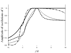
Figure 5: Amplitude of Aharonov-Bohm oscillations vs. $J/k$ for $kL=1$ and in the case of the initial spin states $\left|\uparrow\right\rangle\left|\uparrow\uparrow\right\rangle$ (——), $\left|\uparrow\right\rangle\left|\uparrow\downarrow\right\rangle$ ($\cdot\cdot\cdot\cdot\cdot$), $\left|\uparrow\right\rangle\left|\Psi^{+}\right\rangle$ (— —) and $\left|\uparrow\right\rangle\left|\Psi^{-}\right\rangle$ ($-\cdot\cdot\,-$).

To quantify the above finite range, we introduce the quantity $R$, defined as the width of the interval around $J/K=0$ where the amplitude of AB oscillation for a given initial spin state is larger than $0.95$. To further illustrate how the electron transmission through the ring depends on the state in which the two impurities are prepared let us consider the family of one spin up impurity spins states

$$\left|\Psi(\theta,\varphi)\right\rangle=\cos\theta\left|\uparrow\downarrow\right\rangle+e^{i\varphi}\sin\theta\left|\downarrow\uparrow\right\rangle$$ (10)

with $\theta\in[0,2\pi]$ and $\varphi\in[0,\pi]$. This family includes both maximally entangled and product states. In Fig. 6 we plot $R$ as a function of $\theta$ and $\varphi$ when the electron is injected in the spin state $\left|\uparrow\right\rangle$ and the impurities are prepared in a state (10) for $kL=1$.

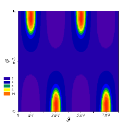
Figure 6: (Color online) $R$ as a function of $\theta$ and $\varphi$ at $kL=1$ when the electron is injected in the up spin state $\left|\uparrow\right\rangle$ with the impurities prepared in the state $\cos{\theta}\left|\uparrow\downarrow\right\rangle+e^{i\varphi}\sin{\theta}\left|\downarrow\uparrow\right\rangle$.

Note how the width of the range showing a nearly coherent behaviour depends crucially on the relative phase $\varphi$ between the impurity spin states $\left|\uparrow\downarrow\right\rangle$ and $\left|\downarrow\uparrow\right\rangle$. Four sharp maxima of $R$ appear in correspondence to the impurity spins prepared in the singlet state $\left|\Psi^{-}\right\rangle$. These results suggests that $\varphi$ can be regarded as a sort of control parameter of electron coherence in a mesoscopic ring with two spin 1/2 impurities.

Such behavior can be explained in terms of an effective quasi-conservation of $\mathbf{S}_{12}^{2}$, where $\mathbf{S}_{12}=\mathbf{S}_{1}+\mathbf{S}_{2}$ denotes the total spin of the two impurities. This observable have quantum number $s_{12}=0,1$, corresponding to the singlet and triplet subspaces, respectively. According to such quasi-conservation, whose origin we will explain shortly, and taking into account the fact that $S_{z}$ is a constant of motion, the initial spin state $\left|\uparrow\right\rangle\left|\Psi^{+}\right\rangle$ is scattered into a linear combination of $\left|\uparrow\right\rangle\left|\Psi^{+}\right\rangle$ and $\left|\downarrow\right\rangle\left|\uparrow\uparrow\right\rangle$. However, since the eigenspace $s_{12}=0$, $m=1/2$ is non degenerate, the initial spin state $\left|\uparrow\right\rangle\left|\Psi^{-}\right\rangle$ is transmitted or reflected nearly unchanged, as shown Fig. 4c. The same of course is true for $\left|\downarrow\right\rangle\left|\Psi^{-}\right\rangle$ and thus for any state $\left(\alpha\left|\uparrow\right\rangle+\beta\left|\downarrow\right\rangle\right)\left|\Psi^{-}\right\rangle$ with arbitrary complex values of $\alpha$ and $\beta$ (this explains why no constraint on the spin polarization of the incoming electron is required). The validity of this quasi-conservation law is further confirmed by Fig. 7 where, for the initial state $\left|\uparrow\right\rangle\left|\Psi^{+}\right\rangle$, we plot the difference between $T$ and the sum of $F$ and $T_{\downarrow\uparrow\uparrow}$, with $T_{\downarrow\uparrow\uparrow}$ being the probability that the system is transmitted in the state $\left|\downarrow\right\rangle\left|\uparrow\uparrow\right\rangle$. A maximum value not larger than 1$\%$ is reached.

Figure 7: $T-F-T_{\uparrow\downarrow\downarrow}$ vs. $\phi/\phi_{0}$ for $kL=1$ and the initial spin state $\left|\uparrow\right\rangle\left|\Psi^{+}\right\rangle$. Solid, dashed and dotted lines stand for $J/k=1,2,5$, respectively.

The origin of quasi-conservation of $\mathbf{S}_{12}^{2}$ can be explained as follows. The wavefunction in the upper arm of the ring is a linear combination of $e^{ik_{1}x}$ and $e^{-ik_{2}x}$, while in the lower one it is linear combination of $e^{ik_{2}x}$ and $e^{-ik_{1}x}$ with $k_{1}=k+(e\phi/\hbar cL)$ and $k_{2}=k-(e\phi/\hbar cL)$ (see Appendix A). This induces an asymmetry between the two arms when a flux $\phi$ is present, since in this case $k_{1}$ differs from $k_{2}$. When $\phi=0$ perfect symmetry holds and $\mathbf{S}_{12}^{2}$ must be rigorously conserved. Indeed, for $\phi=0$ $\left|\uparrow\right\rangle\left|\Psi^{-}\right\rangle$ is transmitted perfectly unchanged (in Fig. 4c $\eta=1$ for $\phi=0$), while $\left|\uparrow\right\rangle\left|\Psi^{+}\right\rangle$ can only either remain unchanged or be flipped into $\left|\downarrow\right\rangle\left|\uparrow\uparrow\right\rangle$ (in Fig. 7 $T-F-T_{\uparrow\downarrow\downarrow}$ exactly vanishes for $\phi=0$). In the presence of a flux $\phi$, the above symmetry is broken and perfect conservation of $\mathbf{S}_{12}^{2}$ generally does not occur. However, even for $\phi\neq 0$ as $kL$ approaches $4n\pi$ ($n=0,1,...$) the symmetry still holds. Indeed, the boundary conditions at the ring junctions and those at the two impurities’ positions imply that the stationary states of the system depend on $kL$ through phase factors of the form $e^{\pm ikL/4}$ and $e^{\pm ikL/2}$ (see Appendix A). It is thus straightforward to see that, for each stationary state, the squared modulus of the wave function is a periodic function of $kL$ with period $4\pi$, this meaning that for $kL=4n\pi$ with $n\neq 0$ the transmission properties of the ring coincide with those obtained for $kL=0$. In the regime $kL=4n\pi$ the system thus behaves as if $k_{1}=-k_{2}=e\phi/\hbar cL$ and the two arms turn out to be symmetric. To illustrate this, in Fig. 8 we plot $R$ versus $kL$ the range $[0,4\pi]$ in the case of the initial spin state $\left|\uparrow\right\rangle\left|\Psi^{-}\right\rangle$. The above mentioned range around $J/k=0$ where a nearly vanishing amplitude reduction takes place shows an increasing width as $kL$ approaches $0$ or $4\pi$ as a signature of an increasing symmetry of the two arms of the ring. For discrepancies between $kL$ and $4n\pi$ up to $0.8\pi$ the width of the coherent range is still appreciable (in Fig. 8 $R>1$ for $kL<0.8\pi$). Good robustness against deviation from the symmetry condition $kL=4n\pi$ is thus exhibited.

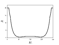
Figure 8: $R$ vs. $kL$ in the case of the initial spin state $\left|\uparrow\right\rangle\left|\Psi^{-}\right\rangle$ for $kL\in[0,4\pi]$.

This also explains why the effect of survival of the AB oscillations’ amplitude for the singlet state of the impurity spins is observable in Figs. 3b and 5 – where we have considered the representative value $kL=1$ – since it turns out that $kL=1\simeq 0.3\,\pi$.

IV Generation of Maximally Entangled States

In this section we mainly address the issue of how to generate the maximally entangled state $\left|\Psi^{-}\right\rangle$ of the two impurity spins giving rise to the above described effects. Possible implementations of a magnetic impurity in the single-channel ring are a paramagnetic impurity atom having a virtual state in the continuum amjphys or a quantum dot with one excess unpaired electron and thus behaving as an effective spin 1/2 system joshi ; ssqc .

Here we propose a method for entangling the two impurities via electron scattering with an entanglement mediator. Generation of entangled states of two magnetic impurities via electron scattering in 1-dimensional systems has been recently investigated in ciccarello ; yang ; yasser ; giorgi ; nakazato .

The basic idea of these schemes is to send an electron in the up spin state $\left|\uparrow\right\rangle$ with the two impurity spins initially in a product state $\left|\downarrow\downarrow\right\rangle$. The impurities are so far apart that their mutual coupling is negligible. The electron interacts with each scatterer via an exchange interaction. $S_{z}$ is conserved in the scattering process and the transmitted spin state will result in a linear combination of $\left|\uparrow\right\rangle\left|\downarrow\downarrow\right\rangle$, $\left|\downarrow\right\rangle\left|\Psi^{+}\right\rangle$ and $\left|\downarrow\right\rangle\left|\Psi^{-}\right\rangle$. If the transmitted electron is filtered in the down spin state $\left|\downarrow\right\rangle$, the two impurities are generally left in an entangled state. This state is not necessarily maximally entangled yasser . However, under conditions allowing $\mathbf{S}_{12}^{2}$ to be an additional constant of motion the above scheme always projects the impurities in the maximally entangled state $\left|\Psi^{+}\right\rangle$ ciccarello . Of course, once $\left|\Psi^{+}\right\rangle$ has been generated, $\left|\Psi^{-}\right\rangle$ can be easily obtained by simply introducing a relative phase shift through a local field acting on one of the two impurities. For our system (Fig. 1), this method works when $\phi=0$ since, as discussed in Sec. III, in this regime both $S_{z}$ and $\mathbf{S}_{12}^{2}$ are strictly conserved. Denoting by $T_{\downarrow}$ the spin polarized probability that the electron is transmitted in the state $\left|\downarrow\right\rangle$ (that is to project the impurities in the state $\left|\Psi^{+}\right\rangle)$, in Fig. 9 we plot $T_{\downarrow}$ versus $J/k$ in the case $kL=1$.

Figure 9: Spin down transmission coefficient $T_{\downarrow}$ at $kL=1$ and $\phi=0$ as a function of $J/k$ when the electron is injected in the state $\left|\uparrow\right\rangle$ with the impurities prepared in the state $\left|\downarrow\downarrow\right\rangle$.

A probability higher than 20$\%$ can be reached with $|J/k|$ lower than 5. In particular, a maximum is exhibited at $J/k\simeq 3$ that is well within the range where the amplitude of AB oscillations for the singlet state is in fact not reduced (see Fig. 5). We have checked that similar behaviors yielding analogous maximum probabilities to generate $\left|\Psi^{+}\right\rangle$ take place for different values of $kL$.

We point out that while in the case of a 1-dimensional wire the above scheme works correctly only for electron wave vectors allowing conservation of $\mathbf{S}_{12}^{2}$ ciccarello , in the present case such constraint is not required. This is due to the previously discussed symmetry of the ring in the absence of an applied flux (see Sec. III).

V Conclusions

In this work, we have considered a mesoscopic ring with two identical spin 1/2 magnetic impurities embedded one in each arm at symmetric locations. Electrons entering the wire undergo multiple scattering by the impurities giving rise to spin-flip processes before being definitively reflected or transmitted. Developing a proper quantum waveguide theory approach based on the coupling of three angular momenta, the exact stationary states and thus all the transmission probability amplitudes of the system in the presence of a magnetic flux have been derived. In agreement with previous studies, we have shown that occurrence of spin-flip events resulting from electron-impurities scattering generally reduces the amplitude of AB oscillations, as a signature of the well-known magnetic impurities induced-electron decoherence. However, an anomalous behaviour appears in the case of the singlet maximally entangled state $\left|\Psi^{-}\right\rangle$ of the impurity spins. At suitable incident electron wave vectors, the amplitude of AB oscillations turns out to be negligibly reduced in a finite range of the electron-impurities coupling constant. At the same time spin-flip turns out to be nearly frozen. This survival of electron coherence via entanglement of the localized spins occurs regardless of the spin state of the incoming electron and thus no constraint on the electron spin polarization is required. Such behaviours have been explained in terms of a quasi-conservation law of the squared total spin of the two impurities. We have proposed a scheme for generating the maximally entangled states $\left|\Psi^{\pm}\right\rangle$ of the two impurities through the same electron scattering mechanism.

In line with the case of a 1-dimensional wire where a perfect resonance condition is always found for two impurities in the state $\left|\Psi^{-}\right\rangle$ ciccarello , we have thus shown how this maximally entangled state is able to effectively “freeze” the usual decoherence due to scattering with magnetic impurities. This phenomenon strongly reminds the so called decoherence free subspaces (DFS), a well-known topic in the study of open quantum systems PalmaSE96 , but usually dealt with for systems encountered in quantum optics. Our work can thus be regarded as a manifestation of DFS in one of the most familiar mesoscopic devices.

Appendix A Derivation of the transmission probability amplitudes

In this Appendix we derive all the transmission probability amplitudes $t_{s_{e2}}^{(s^{\prime}_{e2},s)}$ required for calculating the transmission properties of the system for a given initial spin state $\left|\chi\right\rangle$ according to (7) and (8). This requires the calculation of the stationary states $\left|\Psi_{s^{\prime}_{e2};s,m}\right\rangle$. We basically adopt a quantum waveguide theory approach xia ; mao here properly generalized to take into account the presence of two magnetic impurities. We first consider the subspace $s=3/2$ and then the subspace $s=1/2$.

A.1 Subspace $s=3/2$

In this 4-dimensional subspace ($m=-3/2,...,3/2$), both $s_{e1}$ and $s_{e2}$ can have the only possible value 1. It follows that in this case $\mathbf{S}_{e1}^{2}$ and $\mathbf{S}_{e2}^{2}$ effectively commute and the four stationary states $\left|\Psi_{1;3/2,m}\right\rangle$ belonging to this subspace are thus eigenstates of $\mathbf{S}_{e2}^{2}$ taking the form

$$\left|\Psi_{1;3/2,m}\right\rangle=\left|\varphi\right\rangle\left|1;3/2,m\right\rangle$$ (11)

where $\left|\varphi\right\rangle$ belongs to the electron orbital space. In this case $s_{e2}$ is a good quantum number and coincides with $s^{\prime}_{e2}$. Moreover, the effective form of $H_{ei}$ reads

$$H_{ei}=-J/4\,\delta(x_{i}-L/4)$$ (12)

Eq. (12) shows that in this subspace the two impurities behave as if they were static and thus no spin-flip may occur. The standard case of a ring with two static impurities of Ref. mao is thus recovered. The wave function $\varphi_{i}(x)$ in each segment $i=1,...,6$ (see Fig. 1) nota2 can be easily derived by solving the Schrödinger equation $H_{0}\left|\varphi\right\rangle=E\left|\varphi\right\rangle$ and obtaining xia

$$\varphi_{1}(x) = \alpha_{1}e^{ikx}+\beta_{1}e^{-ikx}$$ (13a)

$$\varphi_{m}(x) = \alpha_{m}e^{ik_{1}x}+\beta_{m}e^{-ik_{2}x}\,\,\,\,\,(m=2,3)$$ (13b)

$$\varphi_{n}(x) = \alpha_{n}e^{ik_{2}x}+\beta_{n}e^{-ik_{1}x}\,\,\,\,\,\,\,\,(n=4,5)$$ (13c)

$$\varphi_{6}(x) = t_{1}^{(1,3/2)}e^{ikx}$$ (13d)

with $k=\sqrt{2m^{*}E}/\hbar$ and

$$k_{1}=k+(e\phi/\hbar cL)$$ (14)

$$k_{2}=k-(e\phi/\hbar cL)$$ (15)

Setting $\alpha_{1}$ to unity, the other unknown coefficients in Eqs. (13a)-(13d) $\alpha$, $\beta$ and the transmission probability amplitude $t_{1}^{(1,3/2)}$ can be determined by imposing proper boundary conditions on the wave function and its derivative at junctions $C$ and $D$ and at the two impurities’ sites xia ; joshi ; mao .

Matching of the wave function at these points as well as conservation of current density at $C$ and $D$ must hold. This yields the following boundary conditions

$$\varphi_{1}(0) = \varphi_{2}(0)$$ (16a)

$$\varphi_{1}(0) = \varphi_{4}(0)$$ (16b)

$$\varphi_{3}(L/2) = \varphi_{6}(0)$$ (16c)

$$\varphi_{5}(L/2) = \varphi_{6}(0)$$ (16d)

$$\varphi_{2}(L/4) = \varphi_{3}(L/4)$$ (16e)

$$\varphi_{4}(L/4) = \varphi_{5}(L/4)$$ (16f)

$$\varphi^{\prime}_{1}(0) = \varphi^{\prime}_{2}(0)+\varphi^{\prime}_{4}(0)$$ (16g)

$$\varphi^{\prime}_{6}(0) = \varphi^{\prime}_{3}(L/2)+\varphi^{\prime}_{5}(L/2)$$ (16h)

On the other hand, at the two impurities’ positions the derivative of the wave function shows a discontinuity due to the $\delta$-like potential (12) according to conditions

$$\varphi^{\prime}_{2}(L/4)-\varphi^{\prime}_{3}(L/4) = \frac{2m^{*}}{\hbar^{2}}\frac{J}{4}\,\varphi_{2}(L/4)$$ (17a)

$$\varphi^{\prime}_{4}(L/4)-\varphi^{\prime}_{5}(L/4) = \frac{2m^{*}}{\hbar^{2}}\frac{J}{4}\,\varphi_{4}(L/4)$$ (17b)

which can be easily derived by integrating the Schrödinger equation across the two impurities’ locations mao .

Boundary conditions (16a)-(16h) and (17a)-(17b) form a linear system in the unknown coefficients appearing in (13a)-(13d). Once this is solved, the transmission amplitude $t_{1}^{(1,3/2)}$ can be obtained. $t_{1}^{(1,3/2)}$ (whose lengthy expression is not shown here) does not depend on $m$ due to the effective form (12) of $H_{ei}$.

A.2 Subspace $s=1/2$

In this 4-dimensional subspace $s_{e1},s_{e2}=0,1$ and thus $\mathbf{S}_{e1}^{2}$ and $\mathbf{S}_{e2}^{2}$ do not commute and $s_{e2}$ is not a good quantum number. This is a signature of the fact that in this space spin-flip may occur. Therefore, for each fixed value of $m=-1/2,1/2$ the stationary states are not eigenstates of $\mathbf{S}_{e2}^{2}$ and take the form

$$\left|\Psi_{s^{\prime}_{e2};1/2,m}\right\rangle=\sum_{s_{e2}=0,1}\left|\varphi_{s^{\prime}_{e2},s_{e2}}\right\rangle\left|s_{e2};1/2,m\right\rangle$$ (18)

where $\left|\varphi_{s^{\prime}_{e2},s_{e2}}\right\rangle$ are orbital wave functions. Note that in the present subspace $s^{\prime}_{e2}\neq s_{e2}$. For fixed $s^{\prime}_{e2}=0,1$ $\left|\Psi_{s^{\prime}_{e2};1/2,m}\right\rangle$ can be found by solving the Schrödinger equation. It is straightforward to see that in each segment $i=1,...,6$ the two wave functions $\varphi_{s^{\prime}_{e2},0}(x)$ and $\varphi_{s^{\prime}_{e2},1}(x)$ turn out to take a form analogous to Eqs. (13a)-(13d). For each of them, continuity of the wave functions as well as conservation of current density at junctions $C$ and $D$ must hold similarly to the case $s=3/2$. However, in this case appropriate boundary conditions on the derivatives of the wave functions at the impurities’sites have to be derived. To do this, we consider the Schrödinger equation at the ring arm containing the $i-$th impurity. This reads

$$\left[\frac{\hbar^{2}}{2m^{*}}\frac{d^{2}}{dx_{i}^{2}}-\frac{1}{2m^{*}}\left(\frac{\xi e\phi}{cL}\right)^{2}+i\frac{\hbar}{m^{*}}\frac{\xi e\phi}{cL}\frac{d}{dx_{i}}+\frac{J}{2}\left(\mathbf{S}_{ei}^{2}-\frac{3}{2}\right)\delta(x_{i}-L/4)+E\right]\Psi_{s^{\prime}_{e2};1/2,m}(x_{i})=0$$

Integration of both sides of Eq. (A.2) across the impurity position yields

$$\left[\Delta\Psi^{\prime}_{s^{\prime}_{e2};1/2,m}(L/4)+\frac{2m^{*}}{\hbar^{2}}\frac{J}{2}\left(\mathbf{S}_{ei}^{2}-\frac{3}{2}\right)\Psi_{s^{\prime}_{e2};1/2,m}(L/4)\right]=0$$ (20)

where $\Delta\Psi^{\prime}_{s^{\prime}_{e2};1/2,m}(L/4)$ stands for the jump of the derivative at the impurity’s site. Once expansion (18) is inserted into Eq. (20) and this is projected onto $\left|0;1/2,m\right\rangle$ and $\left|1;1/2,m\right\rangle$, we obtain the following boundary conditions

$$\Delta\varphi_{s_{e2}^{\prime},0}^{\prime}(L/4) = -\frac{2m^{*}J}{\hbar^{2}}\frac{\sqrt{3}}{4}\,\varphi_{s_{e2}^{\prime},1}(L/4)$$ (21a)

$$\Delta\varphi_{s_{e2}^{\prime},1}^{\prime}(L/4) = \frac{2m^{*}J}{\hbar^{2}}\frac{1}{2}\,\varphi_{s_{e2}^{\prime},1}(L/4)$$ (21b)

$$- \frac{2m^{*}J}{\hbar^{2}}\frac{\sqrt{3}}{4}\,\varphi_{s_{e2}^{\prime},0}(L/4)$$

at impurity 1 and

$$\Delta\varphi_{s_{e2}^{\prime},0}^{\prime}(L/4) = \frac{2m^{*}J}{\hbar^{2}}\frac{3}{4}\,\varphi_{s_{e2}^{\prime},0}(L/4)$$ (22a)

$$\Delta\varphi_{s_{e2}^{\prime},1}^{\prime}(L/4) = -\frac{2m^{*}J}{\hbar^{2}}\,\frac{1}{4}\,\varphi_{s_{e2}^{\prime},1}(L/4)$$ (22b)

at impurity 2. In deriving Eqs. (21a) -(22b) we have used that

$$\langle 0;1/2,m\left|S_{e1}^{2}\right|0;1/2,m\rangle = \frac{3}{2}$$ (23a)

$$\langle 0;1/2,m\left|S_{e1}^{2}\right|1;1/2,m\rangle = \frac{\sqrt{3}}{2}$$ (23b)

$$\langle 1;1/2,m\left|S_{e1}^{2}\right|0;1/2,m\rangle = \frac{\sqrt{3}}{2}$$ (23c)

$$\langle 1;1/2,m\left|S_{e1}^{2}\right|1;1/2,m\rangle = \frac{1}{2}$$ (23d)

The above matrix elements of $\mathbf{S}_{ei}^{2}$ can be easily computed by means of $6j$-coefficients, these allowing to go from the scheme $e2$, where the electron is first coupled to impurity 2, to the $e1$ one.

Note how $\varphi_{s_{e2}^{\prime},0}(x)$ and $\varphi_{s_{e2}^{\prime},1}(x)$ turn out to be mutually coupled by boundary conditions (21a) -(22b). Finally, also taking into account the above mentioned boundary conditions analogous to Eqs. (16a)-(16h), one ends up with a linear system in 20 unknown variables. This can be solved for each $s^{\prime}_{e2}=0,1$ to obtain the transmission amplitudes $t_{0}^{(s^{\prime}_{e2},1/2)}$ and $t_{1}^{(s^{\prime}_{e2},1/2)}$.

Note that these do not depend on $m$ due to the form (5) of $H_{ei}$ and to the fact that $6j$ coefficients and thus matrix elements (23) are $m$-independent (see for instance weissbluth ).

It is important to point out that our calculations yield $t^{(s_{e2}^{\prime};1/2)}_{s_{e2}}\neq 0$ for $s_{e2}\neq s_{e2}^{\prime}$, as a signature of non conservation of $\mathbf{S}_{e2}^{2}$ and definitively of occurrence of spin-flip in the subspace $s=1/2$. The analytical formulas obtained for $t_{0}^{(s^{\prime}_{e2},1/2)}$ and $t_{1}^{(s^{\prime}_{e2},1/2)}$ are quite lengthy and will not be shown here.

- (1) S. Datta, Electronic Transport in Mesoscopic Systems (Cambridge Univ. Press, Cambridge, 1995)
- (2) G. Hackenbroich, Phys. Rep. 343, 463 (2001)
- (3) S. Washburn, and R. A. Webb, Adv. Phys. 35, 375 (1986)
- (4) J.-B. Xia, Phys. Rev. B 45, 3593 (1992)
- (5) Imry Y 1997 Introduction to Mesoscopic Physics (New york: Oxford Univ. Press)
- (6) Stern A, Aharonov Y and Imry Y 1990 Phys. Rev. A 41 3436
- (7) L. S. Schulman, Phys. Lett. A 211, 75 (1996)
- (8) S. K. Joshi, D. Sahoo, and A. M. Jayannavar, Phys. Rev. B 64, 075320 (2001)
- (9) Y.-M. Shi, X.-F. Cao, and H. Chen, Phys. Lett. A 324, 331 (2004)
- (10) J. M. Mao, Y. Huang, and J. M. Zhou, J. Appl. Phys. 73, 1853 (1993)
- (11) F. Ciccarello, G. M. Palma, M. Zarcone, Y. Omar, and V. R. Vieira, New J. Phys. 8, 214 (2006); F. Ciccarello, G. M. Palma, M. Zarcone, Y. Omar and V. R. Vieira, J. Phys. A: Math. Theor. (to be published), ArXiv:quant-ph/0611025
- (12) O. L. T. de Menezes, and J. S. Helman, Am. J. Phys. 53, 1100 (1985)
- (13) Of course, we could also choose the scheme in which the electron is first coupled to impurity 1, while the scheme in which the two impurities are first coupled together is not convenient for the present problem.
- (14) When it is irrelevant to distinguish between different arms of the ring, we denote each local coordinate as .
- (15) M. Weissbluth, Atoms and Molecules (Academic Press, New York, 1978)
- (16) is so denoted since it is actually the fidelity referred to the initial spin state over the transmitted one.
- (17) D. D. Awschalom, D. Loss, and N. Samarth, Semiconductor Spintronics and Quantum Computation (Springer, Berlin, 2002)
- (18) D. Yang, S.-J. Gu, and H. Li, ArXiv:quant-ph/0503131 (2005)
- (19) A. T. Costa, Jr., S. Bose, and Y. Omar, Phys. Rev. Lett. 96, 230501 (2006)
- (20) G. L. Giorgi, and F. De Pasquale, Phys. Rev. B 74, 153308 (2006)
- (21) K. Yuasa, and H. Nakazato, J. Phys. A: Math. Theor. 40, 297 (2007)
- (22) G. M. Palma, K.-A. Suominen, and A. K. Ekert, Proc. R. Soc. Lond. A 452, 567 (1996)