Non-Markovian reduced dynamics and entanglement evolution of two coupled spins in a quantum spin environment

Abstract

The exact quantum dynamics of the reduced density matrix of two coupled spin qubits in a quantum Heisenberg $XY$ spin star environment in the thermodynamic limit at arbitrarily finite temperatures is obtained using a novel operator technique. In this approach, the transformed Hamiltonian becomes effectively Jaynes-Cumming like and thus the analysis is also relevant to cavity quantum electrodynamics. This special operator technique is mathematically simple and physically clear, and allows us to treat systems and environments that could all be strongly coupled mutually and internally. To study their entanglement evolution, the concurrence of the reduced density matrix of the two coupled central spins is also obtained exactly. It is shown that the dynamics of the entanglement depends on the initial state of the system and the coupling strength between the two coupled central spins, the thermal temperature of the spin environment and the interaction between the constituents of the spin environment. We also investigate the effect of detuning which in our model can be controlled by the strength of a locally applied external magnetic field. It is found that the detuning has a significant effect on the entanglement generation between the two spin qubits.

I Introduction

One of the most promising candidates for quantum computation is spin systems 1 ; kane ; 2 ; vrijen ; 3 ; skinner ; ladd ; sousa ; friesen due to their long decoherence and relaxation time . Combined with nanostructure technology, they have the potential advantage to scale up to large systems. Just as other quantum systems, the spin systems are inevitably influenced by their environment, especially the spin environment. As a result, decoherence due to the presence of the environment will cause the transition of a system from pure quantum states to mixed ones. The decoherent behavior of a single spin or several spins interacting with a spin bath has attracted much attention in recent years 4 ; 5 ; 6 ; Schliemann03 . The interaction in such a spin bath system often leads to strong non-Markovian behavior. The usual Markovian quantum master equations which are widely used in the area of atomic physics and quantum optics may fail for many spin bath models. Therefore it becomes more and more important to develop methods that are capable of going beyond the Markovian approximation 7 ; Breuerb ; Hamdouni06 .

Entanglement has been recognized as one of the most amazing aspects of quantum mechanics. It has been considered as important resources for applications in quantum communication and information processing, such as quantum teleportation Bennett1 , quantum cryptography 16 , quantum dense coding 17 , and telecloning 18 . It is also believed to be one of the features that make quantum computers more powerful than classical ones. For spin systems, much attention has been dedicated to the problem of thermal entanglement 21 ; Osborne02 ; 20 , i.e., to quantify entanglement arising in spin chains at thermal equilibrium with an environment or a reservoir. In this approach, a thermal distribution of the system energy levels is determined by the environment temperature, but the detailed interaction between the system and environment, and the evolution of the system toward the thermal equilibrium are explicitly ignored.

A quantum system exposed to environmental modes is described by the reduced density matrix when the environment modes are traced over. The time evolution of the reduced density matrix is usually very difficulty to obtain in the case of non-Markovian process. Recently, the dynamics of the reduced density matrix for one-, two- and three-spin-qubit systems in a spin bath described by the transverse Ising model has been analyzed without making the Markovian approximation, but using a perturbative expansion method Paganelli02 or a mean-field approximation 22 ; Ma05 . The interaction between the system and the spin bath for these cases was assumed to be of a Ising type. It has also been reported recently that the exact reduced dynamics and for one- and two-spin-qubit systems in a spin-star environment 23 has been derived and analyzed 7 ; Breuerb . There, the interaction between the system and environment was assumed to be of a Heisenberg $XY$ interaction.

In this paper, we study a two-spin-qubit system in a spin star configuration, similar to the case studied in Ref. Hamdouni06, . There are however several important differences between our model and that of Ref. Hamdouni06, . In Ref. Hamdouni06, , the interaction between the two-spin qubits and the interaction between the constituents of the spin environment are neglected, i.e., no internal dynamics for both the spin qubit system and the spin environment is considered. In addition, the spin environment is assumed to be initially in an unpolarized infinite temperature state. As a result, no dependence of the environment temperature on the dynamics and entanglement is present. It is under these conditions that the “exact” dynamics is reported in Ref. Hamdouni06, . Neglecting the direct interaction among the constituents in the environment and considering only the infinite temperature initial state may not be proper in dealing with spin baths. In this paper, we investigate a more general case. Using a novel operator technique, we present an exact calculation of the dynamics of the reduced density matrix of two coupled spins interacting with a thermal spin bath at finite temperatures in the thermodynamic limit. In our model, the interaction between the constituents of the spin environment, the interaction between the two spin qubits, and the interaction between the the spin qubit system and the spin environment are all of the Heisenberg $XY$ type and can all be taken into account simultaneously. In addition, we include also the Zeeman coupling between the spin qubits and a locally applied external magnetic field. To quantify quantum entanglement dynamics of the two coupled spins under the influence of the spin bath at arbitrarily finite temperatures in the thermodynamics limit, we calculate the exact time evolution of their concurrence. Our model involves the Heisenberg $XY$ coupling which has extensive applications for various quantum information processing proposals 9 ; 10 ; 11 ; 12 ; 13 ; 14 ; Blais04 ; Sarovar05 . In addition, the transformed Hamiltonian of the total system in our approach becomes effectively Jaynes-Cumming like and thus our analysis is also very relevant to cavity quantum electrodynamics 9 ; 10 ; Blais04 ; Sarovar05 .

The paper is organized as follows. In Sec. II the model Hamiltonian is introduced and the operator technique is employed to obtain the reduced density matrix, taking into account the memory effect of the environment. From the reduced density matrix, the entanglement measure of concurrence of the coupled spin system is calculated in Sec. III. Conclusions are given in Sec. IV.

II Model and Calculations

We consider a two-spin-qubit system interacting with bath spins via a Heisenberg XY interaction. The system and bath are composed of spin-$\frac{1}{2}$ atoms. We restrict ourselves to a star-like configuration with coupling of equal strength, similar to the cases considered in Refs. 7, ; Breuerb, ; 23, . The interactions between bath spins are also of XY type. In Refs. Paganelli02, ; 22, ; Ma05, , a similar but somewhat different type of Ising interactions between the constituents of the spin bath was considered. The Hamiltonian for the total system is

$$H = H_{S}+H_{SB}+H_{B}.$$ (1)

Here, $H_{S}$ and $H_{B}$ are the Hamiltonians of the system and bath respectively, and $H_{SB}$ is the interaction between them Breuerb ; 23 . They can be written as

$$H_{S} = \mu_{0}(S_{01}^{z}+S_{02}^{z})+\Omega\left(S_{01}^{+}S_{02}^{-}+S_{01}^{-}S_{02}^{+}\right),$$ (2)

$$H_{SB} = \frac{g_{0}}{\sqrt{N}}\left[\left(S_{01}^{+}+S_{02}^{+}\right)\sum_{i=1}^{N}S_{i}^{-}+\left(S_{01}^{-}+S_{02}^{-}\right)\sum_{i=1}^{N}S_{i}^{+}\right],$$ (3)

$$H_{B} = \frac{g}{N}\sum_{i\neq j}^{N}\left(S_{i}^{+}S_{j}^{-}+S_{i}^{-}S_{j}^{+}\right),$$ (4)

where $\mu_{0}$ represents the coupling constant between a locally applied external magnetic field in the $z$ direction and the spin qubit system. $\Omega$ is the the coupling constant between two qubit spins. $S_{0i}^{+}$ and $S_{0i}^{-}$ ($i$=1,2) are the spin-flip operators of the qubit system spins, respectively. $S_{i}^{+}$ and $S_{i}^{-}$ are the corresponding operators of the $i$th atom spin in the bath. The indices of the sums for the spin bath run from $1$ to $N$, where $N$ is the number of the bath atoms. $g_{0}$ is the coupling constant between the qubit system spins and bath spins, whereas $g$ is that between the bath spins. Both coupling strengths are rescaled such that the free energy is extensive and a nontrivial finite limit of $N\rightarrow\infty$ exists Breuerb ; 24 .

By using collective angular momentum operators $J_{\pm}=\sum_{i=1}^{N}S_{i}^{\pm}$, we rewrite the Hamiltonians, Eqs. (3) and (4), as

$$H_{SB} = \frac{g_{0}}{\sqrt{2j}}\left[\left(S_{01}^{+}+S_{02}^{+}\right)J_{-}+\left(S_{01}^{-}+S_{02}^{-}\right)J_{+}\right],$$ (5)

$$H_{B} = \frac{g}{2j}\left(J_{+}J_{-}+J_{-}J_{+}\right)-g,$$ (6)

where $j=N/2$ is the length of the pseudo-spin. After the Holstein-Primakoff transformation 25 ,

$$J_{+} = b^{+}\left(\sqrt{2j-b^{+}b}\right),\hskip 5.69054ptJ_{-}=\left(\sqrt{2j-b^{+}b}\right)b,$$ (7)

with $[b,b^{+}]=1$, the Hamiltonian, Eqs. (5) and (6), can be written as

$$H_{SB} = g_{0}\left[\left(S_{01}^{+}+S_{02}^{+}\right)\sqrt{1-\frac{b^{+}b}{N}}b+\left(S_{01}^{-}+S_{02}^{-}\right)b^{+}\sqrt{1-\frac{b^{+}b}{N}}\right],$$ (8)

$$H_{B} = g\left[b^{+}\left(1-\frac{b^{+}b}{N}\right)b+\sqrt{1-\frac{b^{+}b}{N}}bb^{+}\sqrt{1-\frac{b^{+}b}{N}}\right]-g.$$ (9)

In the thermodynamic limit (i.e. $N\longrightarrow\infty$) at finite temperatures, we then have

$$H_{SB} = g_{0}\left[\left(S_{01}^{+}+S_{02}^{+}\right)b+\left(S_{01}^{-}+S_{02}^{-}\right)b^{+}\right],$$ (10)

$$H_{B} = 2gb^{+}b.$$ (11)

Equations (2), (10) and (11) are then effectively equivalent to the Hamiltonian of a Jaynes-Cumming type. They describe two coupled qubits interacting with a single-mode thermal bosonic bath field, so the analysis of the problem is also relevant to cavity quantum electrodynamics quantum information processing proposals 9 ; 10 ; Blais04 ; Sarovar05 . We note here that due to the high symmetry of our model, the coupling to the environment is actually represented by a coupling to a single collective environment spin. After the Holstein-Primakoff transformation and in the thermodynamic limit, this collective environment spin is transformed into a single-mode bosonic thermal field. The effect of this single-mode environment on the dynamics of the two coupled qubits is extremely non-Markovian. This reflects onto, for example, the revival behavior of the reduced density matrix or entanglement evolution of the two coupled spins, which will be shown later. This is different from the usual environment models which consist of very large degrees of freedom (e.g. many bosonic modes) and often cause the reduced dynamics of the system of interest displaying an exponential decay in time behavior. So the Markovian approximation usually used in quantum optics master equation will not work in our model. One may perform perturbation theory for weak-coupling case, but the single-mode environment in our model will not remain in thermal equilibrium state as usually assumed for an environment with very large degrees of freedom in the weak-coupling master equation approach.

Using a special operator technique, we can obtain the exact reduced density matrix for the two coupled qubits by tracing over the degrees of freedom of the bosonic bath at arbitrarily finite temperatures. Reference 19, reported the theoretical results of entanglement dynamics of a coupled two-level atoms interacting with a cavity mode embedded in an effective atomic environment. However the influence of the environmental temperature was not considered. In Ref. 26, , a decoupled two-qubit system interacting with a single-mode thermal field at resonance (i.e., zero detuning) in the context of cavity electrodynamics was studied. There, the dynamics of the reduced density matrix for the two-qubit system is obtained using the method of the Kraus operator representation. In this paper, we use a different approach of operator technique to obtain the exact non-Markovian dynamics of the reduced density matrix for the two-qubit system for our model of Eqs. (2)-(4) with the bath spins in the thermodynamics limit, or equivalently Eqs. (2), (10) and (11). Different from the case considered in Ref. 26, , our model furthermore includes the coupling between the two qubits and investigates the effect of detuning (i.e., the single bosonic bath mode is not necessarily resonant with the qubit transition frequency). The detuning in our model is represented by $(\mu_{0}-2g)$ and it could be controlled by the strength of a locally applied magnetic field, i.e., the $\mu_{0}$ term in Eq. (2). We find that the detuning has a significant effect on the entanglement generation between the two qubits.

We assume the initial density matrix of the total system to be separable, i.e., $\rho(0)=|\psi\rangle\langle\psi|\otimes\rho_{B}$. The density matrix of the spin bath satisfies the Boltzmann distribution, that is $\rho_{B}=e^{-H_{B}/T}/Z$, where $Z={\rm Tr}\left(e^{-H_{B}/T}\right)$ is the partition function, and the Boltzmann constant has been set to one. At absolute zero temperature, no excitation will exist. The bath is in a thoroughly polarized state with all spins down. With the increase of temperatures, the number of spin up atoms increases. Note that in Ref. Hamdouni06, , the non-interacting bath spins are assumed to be initially in the unpolarized infinite temperature state. The most general form of an initial pure state of the two-qubit system is

$$|\psi(0)\rangle=\alpha|00\rangle+\beta|11\rangle+\gamma|01\rangle+\delta|10\rangle,$$ (12)

$$\mbox{with}\quad|\alpha|^{2}+|\beta|^{2}+|\gamma|^{2}+|\delta|^{2}=1.$$ (13)

We might proceed the calculation with this general initial state, but the final analytical solution would, however, be somewhat complicated. For analytical simplicity, in the following we set $\gamma=\delta=0$. We note that the general initial qubit state case can be calculated in a similar way presented below.

By taking the initial state of the two qubit system to be $|\psi\rangle=\alpha|00\rangle+\beta|11\rangle$, the reduced density matrix can be written as

$$\rho_{s}(t) = \frac{1}{Z}|\alpha|^{2}\textrm{tr}_{B}\left[e^{-iHt}|00\rangle e^{-H_{B}/T}\langle 00|e^{iHt}\right]$$ (14)

$$+\frac{1}{Z}\alpha\beta^{*}\textrm{tr}_{B}\left[e^{-iHt}|00\rangle e^{-H_{B}/T}\langle 11|e^{iHt}\right]$$

$$+\frac{1}{Z}\alpha^{*}\beta\textrm{tr}_{B}\left[e^{-iHt}|11\rangle e^{-H_{B}/T}\langle 00|e^{iHt}\right]$$

$$+\frac{1}{Z}|\beta|^{2}\textrm{tr}_{B}\left[e^{-iHt}|11\rangle e^{-H_{B}/T}\langle 11|e^{iHt}\right],$$

where

$$Z=\frac{1}{1-e^{-2g/T}}.$$ (15)

The matrix $\rho_{s}(t)$ is a $4\times 4$ matrix in the standard basis $|00\rangle$, $|01\rangle$, $|10\rangle$, $|11\rangle$. In order to obtain the exact reduced density matrix elements, we have to evaluate Eq. (14) exactly. However, it is difficult to do so using usual methods, because the treated system and environment could all be strongly coupled mutually and internally. In the following, we will present a special operator technique to obtain the exact density matrix elements. As shown below, our treatment is mathematically simple and physically clear, and may be easily extended to more complicated systems with strong coupling. Note also that our method also applies to the case that the two-qubit system is initially in a mixed state. For example, if the initial state for the qubits is $\rho_{s}(0)=|\alpha|^{2}|00\rangle\langle 00|+|\beta|^{2}|11\rangle\langle 11|$, the corresponding reduced density matrix is Eq. (14) provided that the second and third terms on its right hand side are removed.

The basic idea of our operator technique is as follows. Before tracing over the environmental degrees of freedom, we will first convert the time evolution equation of the qubit system under the action of the total Hamiltonian into a set of coupled non-commuting operator variable equations. Then by introducing a new set of transformation on the operator variables, we turn the coupled non-commuting operator variable equations into commuting ones. As a result, they can be solved exactly by using the general method of solving coupled first-order ordinary differential equations for ordinary variables. After that, the trace over the environmental degrees of freedom can be performed and the exact reduced dynamics of the qubit system can be obtained.

From the total Hamiltonian $H$, we can see that it consists of operators $b$, $b^{+}$, $S_{0i}^{-}$ and $S_{0i}^{+}$, where $S_{0i}^{-}$, and $S_{0i}^{+}$ change the $i$th ($i=1,2$) qubit spin from state $|1\rangle_{i}$ to $|0\rangle_{i}$, and vice versa. It is then obvious that we can write in a most general form that

$$e^{-iHt}|11\rangle=A|00\rangle+B|01\rangle+C|10\rangle+D|11\rangle,$$ (16)

where $A$, $B$, $C$, and $D$ are functions of operators $b$, $b^{+}$, and time $t$. Using the Schrödinger equation identity

$$i\frac{d}{dt}\left(e^{-iHt}|11\rangle\right)=H\left(e^{-iHt}|11\rangle\right)$$ (17)

and Eq. (16), we obtain

$$\frac{d}{dt}A = -i\left[-\mu_{0}A+2gb^{+}bA+g_{0}b^{+}B+g_{0}b^{+}C\right],$$ (18)

$$\frac{d}{dt}B = -i\left[g_{0}bA+2gb^{+}bB+\Omega C+g_{0}b^{+}D\right],$$ (19)

$$\frac{d}{dt}C = -i\left[g_{0}bA+\Omega B+2gb^{+}bC+g_{0}b^{+}D\right],$$ (20)

$$\frac{d}{dt}D = -i\left[g_{0}bB+g_{0}bC+\mu_{0}D+2gb^{+}bD\right],$$ (21)

with initial conditions from Eq. (16) being $A(0)=0$, $B(0)=0$, $C(0)=0$, and $D(0)=1$. As $A$, $B$, $C$, $D$ are functions of $b^{+}$ and $b$, they are operators and do not commute with each other. Equations (18)-(21) are thus coupled differential equations of non-commuting operator variables, which can not be solved by using conventional methods for ordinary number variables.

The crucial observation to solve the problem is that the Hamiltonian, Eqs. (2), (10) and (11), is of an effective Jaynes-Cumming type and it can be block-diagonalized in the dressed state subspace of $|i,j;n\rangle$, with $i+j+n={\rm constant}$. Here $|i,j\rangle$ represent the qubit states and $|n\rangle$ are the bosonic field number states. As a result, we may rewrite Eqs. (18)-(21) in such a subspace. By introducing the following transformation

$$A = b^{+}b^{+}e^{-i2g(b^{+}b+1)t}A_{1},$$ (22)

$$B = b^{+}e^{-i2g(b^{+}b+1)t}B_{1},$$ (23)

$$C = b^{+}e^{-i2g(b^{+}b+1)t}C_{1},$$ (24)

$$D = e^{-i2g(b^{+}b+1)t}D_{1},$$ (25)

equations (18)-(21) then become

$$\frac{d}{dt}A_{1} = i(\mu_{0}-2g)A_{1}-ig_{0}\left(B_{1}+C_{1}\right),$$ (26)

$$\frac{d}{dt}B_{1} = -i\left[g_{0}(2+\hat{n})A_{1}+\Omega C_{1}+g_{0}D_{1}\right],$$ (27)

$$\frac{d}{dt}C_{1} = -i\left[g_{0}(2+\hat{n})A_{1}+\Omega B_{1}+g_{0}D_{1}\right],$$ (28)

$$\frac{d}{dt}D_{1} = -ig_{0}(1+\hat{n})\left(B_{1}+C_{1}\right)-i(\mu_{0}-2g)D_{1},$$ (29)

where $\hat{n}=b^{+}b$. Note that for initial qubit state in $|11\rangle$ on the left hand side of Eq. (16), the transformation, Eqs. (22)-(25), is chosen in such a way that the bosonic field operator(s) in front of the exponential term in Eqs. (22)-(25) together with its corresponding qubit state on the right hand side of Eq. (16) make $i+j+n$ a constant value and the initial condition $D(0)=D_{1}(0)=1$. That is, the operator coefficient $A$ of $|00\rangle$ state on the right hand side of Eq. (16) requires two field creation operators in Eq. (22), $B$ and $C$ of $|01\rangle$ and $|10\rangle$ respectively require only one field creation operator in Eqs. (23) and (24), and $D$ of $|11\rangle$ does not need any field operator in Eq. (25). The exponential term in Eqs. (22)-(25) is introduced to make the resultant equations more concise. As a consequence, the coefficients of Eqs. (26)-(29) after the transformation (22)-(25) involve only the operator $\hat{n}$. Therefore $A_{1}$, $B_{1}$, $C_{1}$, and $D_{1}$ are functions of $\hat{n}$ and $t$, and commute with each other. We can then treat Eqs. (26)-(29) as coupled complex-number differential equations and solve them in a usual way. This novel operators approach thus allows us to solve Eq. (16) and then consequently the non-Markovian dynamics of the reduced density matrix of the qubit system.

We note again that the crucial point of the method used here is to find proper transformations to change the coupled differential equations of non-commuting operator variables to the coupled differential equations of complex-number variables. This can be done when the effective Hamiltonian can be block-diagonalized. This is the case of Jaynes-Cumming model and other models which contain interaction Hamiltonian of the forms of, for example, $\left(S_{01}^{+}+S_{02}^{+}\right)bb+\left(S_{01}^{-}+S_{02}^{-}\right)b^{+}b^{+}$, $S_{01}^{+}S_{02}^{+}b+S_{01}^{-}S_{02}^{-}b^{+}$, etc., regardless how strong their interaction strengths are. If the total effective Hamiltonian can not be block-diagonalized, for example, for the effective spin-boson model in Ref. Irish, , the operator method used here will then not apply to solve the problem exactly.

As we are working in the Schrödinger picture, the basic operator $\hat{n}=b^{+}b$ is time independent (sometimes the operators could have time dependence explicitly; however this is not the case here). From Eq. (16) and Eqs. (22)-(25), the initial conditions at $t=0$ are given by

$$A_{1}(0) = 0,$$ (30)

$$B_{1}(0) = 0,$$ (31)

$$C_{1}(0) = 0,$$ (32)

$$D_{1}(0) = 1.$$ (33)

In general, we can solve Eqs. (26)-(29) exactly via the initial conditions Eqs. (30)-(33). As we aim to obtain analytical expressions for the reduced qubit dynamics, for the sake of analytical simplicity we consider the on-resonant case, i.e., $\mu_{0}=2g$. We can easily tune the locally applied external magnetic field to satisfy this condition. We will give the numerical results for the off-resonant case in Fig. 6. We then obtain for the on-resonant case

$$A_{1} = \frac{-1}{3+2\hat{n}}+\frac{2g_{0}^{2}}{\sqrt{\Omega^{2}+8(3+2\hat{n})g_{0}^{2}}}\left[\frac{e^{i\lambda_{1}t}}{\lambda_{1}}-\frac{e^{i\lambda_{2}t}}{\lambda_{2}}\right],$$ (34)

$$B_{1} = C_{1}=-\frac{g_{0}}{\sqrt{\Omega^{2}+8(3+2\hat{n})g_{0}^{2}}}\left[e^{i\lambda_{1}t}-e^{i\lambda_{2}t}\right],$$ (35)

$$D_{1} = \frac{2+\hat{n}}{3+2\hat{n}}+\frac{2g_{0}^{2}(1+\hat{n})}{\sqrt{\Omega^{2}+8(3+2\hat{n})g_{0}^{2}}}\left[\frac{e^{i\lambda_{1}t}}{\lambda_{1}}-\frac{e^{i\lambda_{2}t}}{\lambda_{2}}\right],$$ (36)

where

$$\lambda_{1,2}=\frac{-\Omega\pm\sqrt{\Omega^{2}+8(3+2\hat{n})g_{0}^{2}}}{2}.$$ (37)

Following the similar calculations above, we can evaluate the time evolution for the initial two-qubit spin state of $|00\rangle$. Let

$$e^{-iHt}|00\rangle=E|00\rangle+F|01\rangle+G|10\rangle+K|11\rangle.$$ (38)

In a similar way, we have

$$E = e^{-i2g\left(b^{+}b-1\right)t}E_{1},$$ (39)

$$F = be^{-i2g\left(b^{+}b-1\right)t}F_{1},$$ (40)

$$G = be^{-i2g\left(b^{+}b-1\right)t}G_{1},$$ (41)

$$K = bbe^{-i2g\left(b^{+}b-1\right)t}K_{1},$$ (42)

and then obtain

$$E_{1} = \frac{\hat{n}-1}{2\hat{n}-1}+\frac{2g_{0}^{2}\hat{n}}{\sqrt{\Omega^{2}+8(2\hat{n}-1)g_{0}^{2}}}\left[\frac{e^{i\lambda_{1}^{\prime}t}}{\lambda_{1}^{\prime}}-\frac{e^{i\lambda_{2}^{\prime}t}}{\lambda_{2}^{\prime}}\right],$$ (43)

$$F_{1} = G_{1}=-\frac{g_{0}}{\sqrt{\Omega^{2}+8(2\hat{n}-1)g_{0}^{2}}}\left[e^{i\lambda_{1}^{\prime}t}-e^{i\lambda_{2}^{\prime}t}\right],$$ (44)

$$K_{1} = \frac{-1}{2\hat{n}-1}+\frac{2g_{0}^{2}}{\sqrt{\Omega^{2}+8(2\hat{n}-1)g_{0}^{2}}}\left[\frac{e^{i\lambda_{1}^{\prime}t}}{\lambda_{1}^{\prime}}-\frac{e^{i\lambda_{2}^{\prime}t}}{\lambda_{2}^{\prime}}\right],$$ (45)

where

$$\lambda_{1,2}^{\prime}=\frac{-\Omega\pm\sqrt{\Omega^{2}+8(2\hat{n}-1)g_{0}^{2}}}{2}.$$ (46)

From Eq. (14) and all the results that we obtained, the reduced density matrix can be written as

$$\rho_{s}(t) = \left(\begin{array}[]{cccc}\rho_{11}&0&0&\rho_{14}\\ 0&\rho_{22}&\rho_{23}&0\\ 0&\rho_{32}&\rho_{33}&0\\ \rho_{14}^{*}&0&0&\rho_{44}\\ \end{array}\right),$$ (51)

where

$$\rho_{11} = |\alpha|^{2}\frac{1}{Z}\sum_{n=0}^{\infty}E_{1}E_{1}^{+}e^{-2gn/T}$$ (52)

$$+|\beta|^{2}\frac{1}{Z}\sum_{n=0}^{\infty}A_{1}A_{1}^{+}(n+1)(n+2)e^{-2gn/T},$$

$$\rho_{14} = \alpha\beta^{*}\frac{1}{Z}\sum_{n=0}^{\infty}E_{1}D_{1}^{+}e^{-2gn/T}e^{i4gt},$$ (53)

$$\rho_{22} = \rho_{23}=\rho_{32}=\rho_{33}$$ (54)

$$= |\alpha|^{2}\frac{1}{Z}\sum_{n=1}^{\infty}F_{1}F_{1}^{+}ne^{-2gn/T}$$

$$+|\beta|^{2}\frac{1}{Z}\sum_{n=0}^{\infty}B_{1}B_{1}^{+}(n+1)e^{-2gn/T},$$

$$\rho_{44} = |\alpha|^{2}\frac{1}{Z}\sum_{n=2}^{\infty}K_{1}K_{1}^{+}n(n-1)e^{-2gn/T}$$ (55)

$$+|\beta|^{2}\frac{1}{Z}\sum_{n=0}^{\infty}D_{1}D_{1}^{+}e^{-2gn/T}.$$

In Eqs. (48)-(51), the trace over the environmental degrees of freedom has been performed and the operator $\hat{n}$ has been replaced by its eigenvalue $n$. In a similar way, the solutions for the reduced dynamics of the two-coupled spins under the influence of the quantum Heisenberg $XY$ spin star bath in the thermal dynamics limit at arbitrarily finite temperatures for arbitrary initial states of $|\psi(0)\rangle=\alpha|00\rangle+\beta|11\rangle+\gamma|01\rangle+\delta|10\rangle$ can be obtained.

III Concurrence and Entanglement Dynamics

We use the concurrence 27 to measure the entanglement between the two coupled qubit spins. It is defined as 27

$$C_{12}=\textrm{max}\{\lambda_{1}-\lambda_{2}-\lambda_{3}-\lambda_{4},0\},$$ (56)

where the quantities $\lambda_{1}\geq\lambda_{2}\geq\lambda_{3}\geq\lambda_{4}$ are the square roots of the eigenvalues of the operator

$$R_{12}=\rho_{s}\left(\sigma^{y}\otimes\sigma^{y}\right)\rho_{s}^{*}\left(\sigma^{y}\otimes\sigma^{y}\right).$$ (57)

We find $\lambda_{i}$ are values in decreasing order of $\sqrt{\rho_{11}\rho_{44}}+|\rho_{14}|$, $|\sqrt{\rho_{11}\rho_{44}}-|\rho_{14}||$, $2\rho_{22}$, and $0$. For the system with an initial state of $|\psi\rangle=|00\rangle$, i.e., the both spins in the ground state, we plot the time evolution of the concurrence in Fig. 1. Although there is no initial entanglement and no coupling between the two spins, it is interesting to notice that the entanglement between the two spins after some time is present as shown in Fig. 1(a). This confirms that the environment which usually causes the decoherence of the system can nevertheless entangle qubits that are initially prepared in a separable state 26 ; 28 ; 29 ; 30 ; Napoli . This is mainly due to the fact that the two spins are coupled to the same, common environment which then in turn generates some effective interaction between the two spins even if they were originally decoupled. The result, however, depends on the environmental temperature. Further numerical calculations show that no entanglement is generated, for example, for $T>8g$. As the coupling between the two qubit spins is switched on even though the value is small, the “collapse” and “revival” of the entanglement as a function of time are demonstrated in Fig. 1(b). This is in analogy to the collapse and revival of atomic population inversion of a single two-level atom interacting with a single mode field initially in a coherent state 31 , a Fock state 19 or a squeezed state Fleischhauer93 in quantum optics. Here from the Hamiltonian, Eqs. (2), (10) and (11), this novel phenomenon of entanglement arises from two-coupled qubits interacting with a single mode field initially however in a thermal state. The reasons for causing the collapse and revival behaviors in these cases could be similar, that is the Rabi (or time evolution) oscillations associated with different excitations have different frequencies . Consequently, as the time increases, these Rabi (or time evolution) oscillations become uncorrelated leading to a collapse behavior. As time is further increased, the correlation is restored and the revival occurs.

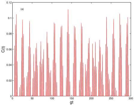
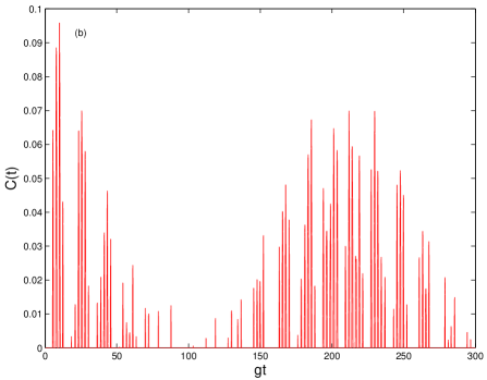
Figure 1: (color online) Time evolution of concurrence for an initial two-qubit state of $|\psi\rangle=|00\rangle$ for different values of $\Omega$; (a) $\Omega=0$ and (b) $\Omega=0.03g$. Other parameters are $\mu_{0}=2g$, $g_{0}=g$, $T=1g$.

Figure 2 shows the time evolution of the concurrence for the system in the initial state of $|\psi\rangle=\frac{1}{\sqrt{2}}(|00\rangle+|11\rangle)$, i.e., an maximally entangled state. At high temperature, the state loses its entanglement completely for a short period of time, and then it is partially entangled again some times later. This is in agreement with the results of Ref. Hamdouni06, where an initially unpolarized infinitely temperature states of the spin bath is assumed. However, our results are temperature dependent. At a very low temperature, the concurrence exhibits the behavior of oscillation between 1 and 0.35. With increasing temperatures, the concurrence decreases more quickly and oscillates disorderly in the lower value region. At a fixed time $t$, the concurrence decreases with temperatures and a critical temperature $T_{c}$ exists, above which the entanglement vanishes. However, this critical temperature $T_{c}$ is time-dependent and sensitive to the initial state of the system. Figure 3 illustrates the time evolutions of the concurrence for different values of the coupling constant $g_{0}$. As expected, increasing the value of the coupling constant has similar effects as increasing the value of the environmental temperature, i.e., the decay rate of the concurrence increases. Figure 4 presents the time evolution of the concurrence for different inner-bath-spin coupling constants $g$. We see that the concurrence increases with the increase of $g$. This confirms that strong quantum correlations within the environment suppress decoherence Paganelli02 ; Tessieri03 ; Dawson05 and thus perhaps also disentanglement. As shown in the inset, the concurrence is regained sometime later. However, it appears disorderly without a particular pattern. Similar behaviors arise for Fig. 2, Fig. 3, and Fig. 5 in the long time scales, which reflect the Non-Markovian dynamics of the system. In Fig. 5, we show the effect of the coupling between the two qubit spins on the concurrence. It is obvious that the coupling benefits the entanglement. Note that the initial state of the system in this case is different from that in Fig. 1. So, if the system is initially prepared in a maximally entangled state, the larger the coupling constant $\Omega$ is, the more slowly the entanglement decays.

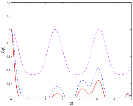
Figure 2: (color online) Time evolution of concurrence for an initial two-qubit state of $|\psi\rangle=\frac{1}{\sqrt{2}}(|00\rangle+|11\rangle)$ for different temperatures; $T=10g$ (solid curve), $T=5g$ (dashed curve) and $T=0.1g$ (dot dashed curve). Other parameters are $\mu_{0}=2g$, $g_{0}=g$, $\Omega=0$.

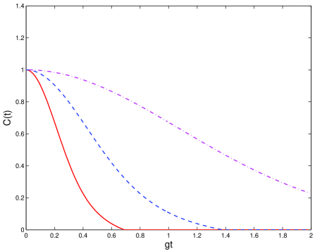
Figure 3: (color online) Time evolution of concurrence for an initial two-qubit state of $|\psi\rangle=\frac{1}{\sqrt{2}}(|00\rangle+|11\rangle)$ for different values of $g_{0}$; $g_{0}=g$ (solid curve), $g_{0}=0.5g$ (dashed curve) and $g_{0}=0.2g$ (dot dashed curve). Other parameters are $\mu_{0}=2g$, $T=5g$, $\Omega=0$.

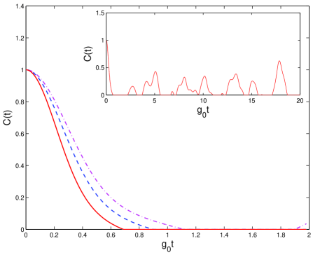
Figure 4: (color online) Time evolution of concurrence for an initial two-qubit state of $|\psi\rangle=\frac{1}{\sqrt{2}}(|00\rangle+|11\rangle)$ for different values of $g$; $g=g_{0}$ (solid curve), $g=1.5g_{0}$ (dashed curve) and $g=2g_{0}$ (dot dashed curve). Other parameters are $\mu_{0}=2g$, $T=5g_{0}$, $\Omega=0$. The inset shows the long time behavior of concurrence for $g=g_{0}$.

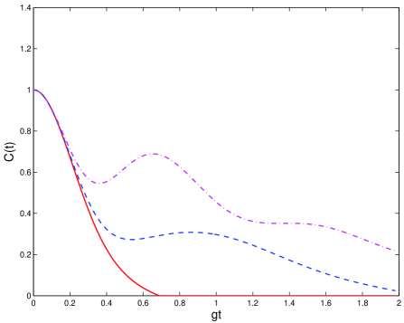
Figure 5: (color online) Time evolution of concurrence for an initial two-qubit state of $|\psi\rangle=\frac{1}{\sqrt{2}}(|00\rangle+|11\rangle)$ for different values of $\Omega$; $\Omega=0$ (solid curve), $\Omega=3g$ (dashed curve), and $\Omega=6g$ (dot dashed curve). Other parameters are $\mu_{0}=2g$, $g_{0}=g$, $T=5g$.

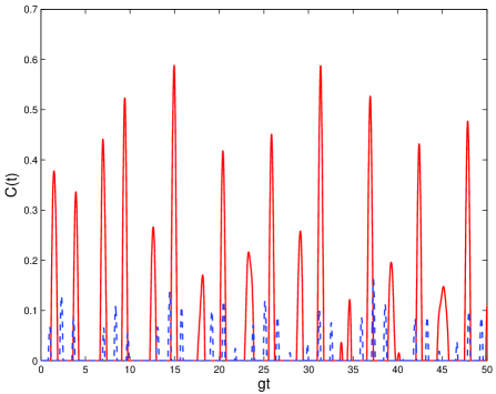
Figure 6: (color online) Time evolution of concurrence for an initial two-qubit state of $|\psi\rangle=|11\rangle$ for different values of detuning; $\mu_{0}=3.5g$ (solid curve), and $\mu_{0}=6g$ (dashed curve). Other parameters are $g_{0}=g$, $T=1g$, $\Omega=0$.

When the two spins are initially prepared in their excited state, i.e. $|\psi\rangle=|11\rangle$, the result is quiet different from that in Fig. 1. If the detuning $\mu_{0}=2g$, i.e., at the on-resonant case, no entanglement between the two qubit spins exists at any temperatures, even with a strong interaction $\Omega$ between them. This is consistent with the result for two qubit atoms obtained by Kim et al., 26 where the coupling between the two qubit atoms is not considered and the detuning between the two atoms and the single-mode field is zero. If the detuning $\mu_{0}\neq 2g$, i.e., in the off-resonant case, the two qubit spins will entangle via the environment again as shown in Fig. 6. So the entanglement generation of the two spins in this case is very sensitive to the detuning which can be controlled in our model by the locally applied external magnetic field.

IV Conclusion

We have studied the exact entanglement evolution of two coupled qubit spins in a model of a quantum Heisenberg $XY$ spin star environment in the thermodynamic limit. The dynamics of the reduced density matrix of the two coupled spins is analytically obtained in terms of a novel operator technique which is mathematically simple and physically clear. In our analysis, the transformed Hamiltonian becomes effectively Jaynes-Cumming like and thus the results are also relevant to cavity quantum electrodynamics.

The time evolutions of the concurrence of the two coupled spin qubits for different initial conditions are evaluated exactly. The results show that the dynamics of the entanglement strongly depends on the initial state of the system, the coupling between the two spin qubits, the interaction between the qubit system and the environment, the interactions between the constituents of the spin environment, the environmental temperatures, as well as the detuning controlled by a locally applied external magnetic field. We have also found that if the two coupled spin qubits are initially prepared in the ground state, the entanglement between them will exhibit the “collapse” and “revival” behavior with time due to the interaction between the two spin qubits and the environment, in analogy to the collapse and revival of the atomic population inversion in quantum optics.

- (1) D. Loss and D. P. DiVincenzo, Phys. Rev. A 57, 120 (1998).
- (2) B. E. Kane, Nature 393, 133 (1998).
- (3) G. Burkard, D. Loss, and D. P. DiVincenzo, Phys. Rev. B 59, 2070 (1999).
- (4) R. Vrijen, E. Yablonovitch, K. Wang, H. W. Jiang, A. Balandin, V. Roychowdhury, T. Mor, and D. DiVincenzo, Phys. Rev. A 62, 012306 (2000).
- (5) R. Raussendorf and H.J. Briegel, Phys. Rev. Lett. 86, 5188 (2001).
- (6) A. J. Skinner, M. E. Davenport, and B. E. Kane, Phys. Rev. Lett. 90, 087901 (2003).
- (7) T. D. Ladd, J. R. Goldman, F. Yamaguchi, Y. Yamamoto, E. Abe, and K. M. Itoh, Phys. Rev. Lett. 89, 017901 (2002).
- (8) R. de Sousa, J. D. Delgado, and S. Das Sarma, Phys. Rev. A 70, 052304 (2004).
- (9) M. Friesen, P. Rugheimer, D. E. Savage, M. G. Lagally, D. W. van der Weide, R. Joynt, and M. A. Eriksson, Phys. Rev. B 67, 121301(R) (2003).
- (10) W. H. Zurek, Rev. Mod. Phys. 75, 715 (2003).
- (11) A. Melikidze, V. V. Dobrovitski, H. A. De Raedt, M. I. Katsnelson, and B. N. Harmon, Phys. Rev. B 70, 014435 (2004).
- (12) N. V. Prokof’er and P. C. E. Stamp, Rep. Prog. Phys. 63, 669 (2000).
- (13) J. Schliemann, A. Khaetskii, and D. Loss, J. Phys.: Condens Matter 15, R1809 (2003).
- (14) H. P. Breuer, Phys. Rev. A 69, 022115 (2004).
- (15) H. P. Breuer, D. Burgarth, and F. Petruccione, Phys. Rev. B 70, 045323 (2004).
- (16) Y. Hamdouni, M. Fannes, and F. Petruccione, Phys. Rev. B 73, 245323 (2006).
- (17) C. H. Bennett, G. Brassard, C. Crépeau, R. Jozsa, A. Peres, and W. K. Wootters, Phys. Rev. Lett. 70, 1895 (1993).
- (18) C. H. Bennett, G. Brassard, and A. K. Ekert, Sci. Am. (Int. Ed.) 267, 50 (1992).
- (19) C. H. Bennett and S. J. Wiesner, Phys. Rev. Lett. 69, 2881 (1992).
- (20) M. Murao, D. Jonathan, M.B. Plenio, and V. Vedral, Phys. Rev. A 59, 156 (1999).
- (21) D. Gunlycke, V. M. Kendon, V. Vedral, and S. Bose, Phys. Rev. A 64, 042302 (2001).
- (22) T. J. Osborne and M. A. Nielsen, Phys. Rev. A 66, 032110 (2002).
- (23) N. Canosa and R. Rossignoli, Phys. Rev. A 73, 022347 (2006).
- (24) S. Paganelli, F. de Pasquale, and S. M. Giampaolo, Phys. Rev. A 66, 052317 (2002).
- (25) M. Lucamarini, S. Paganelli, and S. Mancini, Phys. Rev. A 69, 062308 (2004).
- (26) X. San Ma, A. Min Wang, X. Dong Yang, and H. You, J. Phys. A 38, 2761 (2005).
- (27) A. Hutton and S. Bose, Phys. Rev. A 69, 042312 (2004).
- (28) A. Imamoḡlu, D. D. Awschalom, G. Burkard, D. P. DiVincenzo, D. Loss, M. Sherwin, and A. Small, Phys. Rev. Lett. 83, 4204 (1999).
- (29) S. B. Zheng and G. C. Guo, Phys. Rev. Lett. Phys. 85, 2392 (2000).
- (30) D. A. Lidar and L. A. Wu, Phys. Rev. Lett. 88, 017905 (2002).
- (31) L. A. Wu, D. A. Lidar, and M. Friesen, Phys. Rev. Lett. 93, 030501 (2004).
- (32) X. Wang, Phys. Rev. A 64, 012313 (2001).
- (33) C. D. Hill and H.-S. Goan, Phys. Rev. A 68, 012321 (2003).
- (34) A. Blais, R.-S. Huang, A. Wallraff, S. M. Girvin, and R. J. Schoelkopf, Phys. Rev. A 69, 062320 (2004).
- (35) M. Sarovar, H. -S. Goan, T. P. Spiller, and G. J. Milburn, Phys. Rev. A 72, 062327 (2005).
- (36) M. Frasca, Ann. Phys. 313, 26 (2004).
- (37) T. Holstein and H. Primakoff, Phys. Rev. 58, 1098 (1949).
- (38) I. Sainz, A. B. Klimov, and Luis Roa, Phys. Rev. A 73, 032303 (2006).
- (39) M. S. Kim, J. Lee, D. Ahn, and P. L. Knight, Phys. Rev. A 65, 040101(R) (2002).
- (40) E. K. Irish, J. Gea-Banacloche, I. Martin, and K. C. Schwab, Phys. Rev. B 72, 195410 (2005).
- (41) S. Hill and W. K. Wootters, Phys. Rev. Lett. 78, 5022 (1997); W.K. Wootters, ibid 80, 2245 (1998).
- (42) S. Bose, I. Fuentes-Guridi, P. L. Knight, and V. Vedral, Phys. Rev. Lett. 87, 050401 (2001).
- (43) F. Benatti, R. Floreanini, and M. Piani, Phys. Rev. Lett. 91, 070402 (2003).
- (44) M. B. Plenio and S. F. Huelga, Phys. Rev. Lett. 88, 197901 (2002).
- (45) A. Napoli, F. Palumbo, and A. Messina, Journal of Physics: Conference Series 36, 154 (2006).
- (46) M. O. Scully and M. S. Zubairy, Quantum Optics, (Cambridge University Press, Cambridge, 1997).
- (47) M. Fleischhauer and W. P. Schleich, Phys. Rev. A 47, 4258 (1993).
- (48) L. Tessieri and J. Wilkie, J. Phys. A 36, 12305 (2003).
- (49) C. M. Dawson, A. P. Hines, R. H. McKenzie, and G. J. Milburn, Phys. Rev. A 71, 052321 (2005).