[

Charge Gap in the One-Dimensional Extended Hubbard Model at Quarter Filling

Abstract

We propose a new combined approach of the exact diagonalization, the renormalization group and the Bethe ansatz for precise estimates of the charge gap $\Delta$ in the one-dimensional extended Hubbard model with the onsite and the nearest-neighbor interactions $U$ and $V$ at quarter filling. This approach enables us to obtain the absolute value of $\Delta$ including the prefactor without ambiguity even in the critical regime of the metal-insulator transition (MIT) where $\Delta$ is exponentially small, beyond usual renormalization group methods and/or finite size scaling approaches. The detailed results of $\Delta$ down to of order of $10^{-10}$ near the MIT are shown as contour lines on the $U$-$V$ plane.

]

There has been much theoretical interest in the one-dimensional (1D) strongly correlated electron systems such as the $t$-$J$ model and the Hubbard model as a good testing ground for the concept of the Tomonaga-Luttinger liquid [1, 2]. Various methods, such as the weak coupling theory (g-ology), the bosonization theory, the Bethe ansatz (BA) method, the conformal field theory and the numerical approaches have been used to clarify the nature of these models [3]. Among them, combined approaches of the exact diagonalization (ED) and the renormalization group (RG) methods have been extensively developed to investigate the critical behavior near the quantum critical point [4, 5, 6, 7, 8, 9]. These approaches enable us to obtain accurate results of the phase boundary for the spin gap phase and those for the charge gap phase beyond the purely numerical approaches combined with the usual finite size scaling.

Recently, we have intensively examined the critical behavior near the metal-insulator transition (MIT) in the one-dimensional extended Hubbard model with the on-site and the nearest-neighbor interactions $U$ and $V$ at quarter filling using a combined approach of the ED and RG methods [7, 8, 9]. In this approach, the Luttinger-liquid parameter $K_{\rho}$ is calculated by using the ED for finite size systems and is substituted into the RG equation as an initial condition to obtain $K_{\rho}$ in the infinite size system. The obtained result agrees very well with the available exact result for $U=\infty$ even in the critical regime of the MIT where the characteristic energy becomes exponentially small and the usual finite size scaling is not applicable. When the system approaches the MIT critical point $V\to V_{c}$ for a fixed $U$, $K_{\rho}$ behaves as $(K_{\rho}-\frac{1}{4})^{2}=c_{K}(1-V/V_{c})$, where the critical value $V_{c}$ and the coefficient $c_{K}$ are functions of $U$ [9]. This approach also yields the critical behavior of the charge gap $\Delta$ in the insulating state near the MIT, where $|\ln\Delta|^{-2}=c_{\Delta}(V/V_{c}-1)$ with the coefficient $c_{\Delta}$ which is a function of $U$. In these studies [7, 8, 9], however, the absolute value of $\Delta$ including prefactor was not explicitly obtained.

In general, it is considered to be difficult for the RG method or its derivative method to yield absolute value of physical quantities including prefactor. To overcome this difficulty, we join the BA method to our previous combined approach of the ED and the RG methods in the present study. More explicitly, the BA result in the infinite size system with $U=\infty$ is connected to the ED result in the finite size system with finite $U$ through the analysis of the RG solution. The new combined approach enables us to estimate the absolute value of $\Delta$ including the prefactor without ambiguity in contrast to the previous combined approaches.

The extended Hubbard model is given by the following Hamiltonian

$$H = -t\sum_{i,\sigma}(c_{i\sigma}^{\dagger}c_{i+1\sigma}+h.c.)$$ (1)

$$+ U\sum_{i}n_{i\uparrow}n_{i\downarrow}+V\sum_{i,\sigma\sigma^{\prime}}n_{i\sigma}n_{i+1\sigma^{\prime}},$$ (2)

where $c^{\dagger}_{i\sigma}$ stands for the creation operator for an electron with spin $\sigma$ at site $i$ and $n_{i\sigma}=c_{i\sigma}^{\dagger}c_{i\sigma}$. $t$ represents the transfer energy between the nearest-neighbor sites and is set to be unity ($t$=1) in the present study. It is well known that this Hamiltonian eq. (2) can be mapped on an $XXZ$ quantum spin Hamiltonian in the limit $U\rightarrow\infty$. The term of the nearest-neighbor interaction $V$ corresponds to the $Z$-component of the antiferromagnetic exchange coupling and the transfer energy $t$ corresponds to the $X$-component of that. When the $Z$-component is larger than the $X$-component, the system has a ”Ising”-like symmetry and an excitation gap exists. For the Hubbard model, this corresponds to the case with $V>2t$ where the exact result of the charge gap is given by [10]

$$\Delta=4(\sinh\lambda)\sum_{n=-\infty}^{\infty}\frac{(-1)^{n}}{2\cosh n\lambda}$$ (3)

with

$$\lambda=-\ln(V/2-\sqrt{(V/2)^{2}-1)}).$$ (4)

On the other hand, in the case with ”$XY$”-like symmetry ($V<2t$), the system is metallic and the Luttinger-liquid parameter $K_{\rho}$ is exactly obtained by $\cos(\frac{\pi}{4K_{\rho}})=-V/2$ [11].

In order to introduce our approach, we briefly discuss a general argument for 1D-electron systems based on the bosonization theory [1, 2, 3]. According to this theory, the effective Hamiltonian for the 1D electron systems can be generally separated into the charge and spin parts. Therefore, we turn our attention to only the charge part and do not consider the spin part in this work. In the low energy limit, the effective Hamiltonian of the charge part is given by

$$H_{\rho} = \frac{v_{\rho}}{2\pi}\int_{0}^{L}{\rm d}x\left[K_{\rho}(\partial_{x}\theta_{\rho})^{2}+K_{\rho}^{-1}(\partial_{x}\phi_{\rho})^{2}\right]$$ (5)

$$+ \frac{2g_{3\perp}}{(2\pi\alpha)^{2}}\int_{0}^{L}{\rm d}x\cos[2\sqrt{8}\phi_{\rho}(x)],$$ (6)

where $v_{\rho}$ and $K_{\rho}$ are the charge velocity and the coupling parameter, respectively. The operator $\phi_{\rho}$ and the dual operator $\theta_{\rho}$ represent the phase fields of the charge part. $g_{3\perp}$ denotes the amplitude of the umklapp scattering and $\alpha$ is a short-distance cutoff. On the basis of the Hamiltonian eq. (6), the electronic state is described by only the two parameters $K_{\rho}$ and $g_{3\perp}$ except for the energy scale determined by $v_{\rho}$.

At quarter filling, the $8k_{F}$ umklapp scattering plays the crucial effect for the charge gap. The effect of the umklapp term is renormalized under the change of the cutoff $\alpha\rightarrow{\rm e}^{\ell}\alpha$, where $\ell$ is the scaling quantity. This process is also considered as the change of the system size $L\to{\rm e}^{\ell}L$. Therefore, the size dependence of $K_{\rho}$ is described by the RG equations.[7, 8, 9] In this work, we adopt the Kehrein’s formulation as the RG equations [13, 14]

$$\frac{{\rm d}K_{\rho}(\ell)}{{\rm d}\ell} = -8\frac{G(\ell)^{2}K_{\rho}(\ell)^{2}}{\Gamma(8K_{\rho}(\ell)-1)},$$ (7)

$$\frac{{\rm d}\log G(\ell)}{{\rm d}\ell} = [2-8K_{\rho}(\ell)],$$ (8)

where $\Gamma(x)$ is $\Gamma$-function and $G(l)$ stands the umklapp effect with $G(0)=g_{3\perp}/(2\pi v_{\rho})$. Here, the value of the short-distance cutoff $\alpha$ is selected to a lattice constant of the system and set to be unity. This formulation is an extension of the perturbative RG theory and allows us to estimate the charge gap beyond the weak coupling regime.

To solve the RG equations concretely, we need an initial condition for the two values: $K_{\rho}(0)$ and $G(0)$. Because it is easy for the ED calculation to obtain $K_{\rho}(\ell)$ as compared to $G(\ell)$, we eliminate $G(\ell)$ in the RG equations. For this purpose, we integrate eq. (8) to yield

$$G(\ell)=G(\ell_{1})e^{\int_{\ell_{1}}^{\ell}[2-8K_{\rho}(\ell^{\prime})]d\ell^{\prime}},$$ (9)

where $\ell_{1}$ is a constant. Substituting eq. (9) into eq. (7), we obtain the differential equation for $K_{\rho}(\ell)$ as

$$\frac{{\rm d}K_{\rho}(\ell)}{{\rm d}\ell}=-8\frac{G^{2}(\ell_{1})e^{\int_{\ell_{1}}^{\ell}[4-16K_{\rho}(\ell^{\prime})]d\ell^{\prime}}K_{\rho}(\ell)^{2}}{\Gamma(8K_{\rho}(\ell)-1)}.$$ (10)

Setting $K_{\rho}(\ell_{1})$ as the initial condition, we solve eq. (10) numerically except the constant $G(\ell_{1})$. The value of $G(\ell_{1})$ is determined by comparing the solution $K_{\rho}(\ell)$ at $\ell=\ell_{2}$ with the initial value $K_{\rho}(\ell_{2})$. Then, the solutions for eqs. (7) and (8) are completely obtained.

Using the relation $\ell\simeq\ln L$, we calculate two initial values $K_{\rho}(\ell_{1})$ and $K_{\rho}(\ell_{2})$ with $L_{1}$- and $L_{2}$-site systems by the ED method. In the finite size systems, $K_{\rho}(L)$ is calculated by the charge susceptibility $\chi_{c}$ and the Drude weight $D$ by

$$K_{\rho}=\frac{1}{2}(\pi\chi_{c}D)^{1/2}$$ (11)

with $D=\frac{\pi}{L}\frac{\partial^{2}E_{0}(\phi)}{\partial\phi^{2}}$ , where $E_{0}(\phi)$ is the total energy of the ground state as a function of a magnetic flux $L\phi$ and $L$ is the system size [3]. Here, the magnetic flux is imposed by introducing the following gauge transformation: $c_{m\sigma}^{\dagger}\to e^{im\phi}c_{m\sigma}^{\dagger}$ for an arbitrary site $m$. The uniform charge susceptibility $\chi_{c}$ is obtained from

$$\chi_{c}=\frac{4/L}{E_{0}(N+2,L)+E_{0}(N-2,L)-2E_{0}(N,L)},$$ (12)

where $E_{0}(N,L)$ is the ground state energy of a system with $L$ sites and $N$ electrons. Here, the filling $n$ is defined by $n=N/L$. We numerically diagonalize the Hamiltonian eq. (2) up to 16 sites system using the standard Lanczos algorithm. In the case with $U=\infty$, we also calculate $E_{0}(N,L)$ by using the Bethe ansatz method[12] for finite size systems up to 800 sites system. Using the definitions of eqs. (11) and (12), we calculate $K_{\rho}$ and $\chi_{c}$ from the ground state energy of the finite size system.

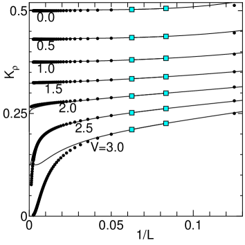
FIG. 1.: The size dependence of $K_{\rho}(L)$ obtained from the RG equations (solid lines) and the exact Bethe ansatz results (filled circles) for various $V$ at $U=\infty$. The shadowed squares are the numerical initial conditions with $L_{1}=12$ and $L_{2}=16$ for the RG equations.

In Fig. 1, we show the size dependence of $K_{\rho}(L)$ obtained from the solutions of the RG equations together with the exact Bethe ansatz results for various $V$ at $U=\infty$. We choose $L_{1}=12$ and $L_{2}=16$ for the numerical initial condition in the RG equations, and we set $L_{1}=L_{2}-4$ hereafter. The limit $K_{\rho}(L\to\infty)$ of the BA result becomes a finite value for $V\leq 2$ and converges to zero for $V>2$. We see that the RG solution is very close to the exact result and the size dependence of $K_{\rho}(L)$ is well described by the RG equations except very large size systems for $V>2$.

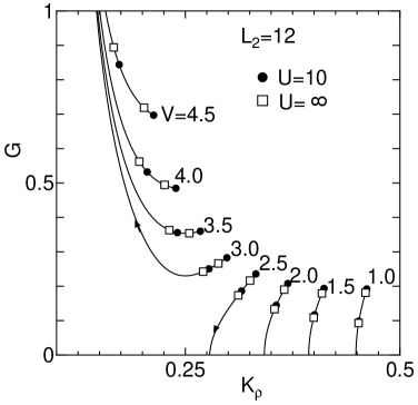
FIG. 2.: The RG flow on the $K_{\rho}-G$ plane for various $V$ at $U=10$ with the numerical initial condition (filled circles). The open squares are the numerical initial condition at $U=\infty$ fitting to the RG flow for $U=10$.

In Fig. 2, we show the RG flows of the systems with various $V$ for $U=10$ together with those for $U=\infty$. We observe that the RG flows for $U=10$ and those for $U=\infty$ coincide to each other. Based on the Luttinger liquid theory, it is considered that the systems assigned by the same RG flows have the same electronic state except energy scale $v_{\rho}$. If we find out a RG flow for $U=\infty$ (we call it a reference system) corresponding to that for finite $U$ (it is a original system), we can connect both systems through the RG flow and derive properties of the original system from the known result of the reference system. To identify the RG flow, we use a renormalized coupling constant $\tilde{G}(\ell)$ constructed by the product of $G(\ell)$ and the effective energy scale $e^{-\ell(2-8K_{\rho})}$. In the limit $\ell\to\infty$, $G(\ell)$ diverges in proportional to $e^{\ell(2-8K_{\rho})}$ (see eq. (9)), while $\tilde{G}(\infty)$ remains a finite value and it becomes a unique index characterizing the RG flow.

Here, we determine the nearest neighbor repulsion $V$ in the reference system with $U=\infty$ so as to fit the RG flow of the reference system to that of the original system with original’s $V$ for a finite value of $U$. The reference’s parameters $V$ corresponding to the several original’s parameters $V$ for $U=10$ are shown in Table I. The reference’s $V$ is smaller than the corresponding original’s $V$. This suggests that the on-site repulsion $U$ causes the renormalization of the nearest neighbor repulsion $V$. Fig.2 also shows that the point indicating the initial condition of the reference system is located at downstream than that of the original system on the RG flow. This means that the effective size of the reference system is larger than the original system size.

TABLE I.: The original’s and the reference’s parameters $V$ for $U=10$ (see in the text).

Original’s $V$	1.0	1.5	2.0	2.5	3.0	3.5	4.0
Reference’s $V$	0.38	0.85	1.33	1.84	2.38	2.92	3.43

Substituting the reference’s $V$ into eq. (4), we obtain the charge gap $\Delta_{\rm r}$ of the reference system from eq. (3). Taking into account the difference of the energy scale, i.e., the charge velocity between the original and the reference systems, we estimate the charge gap of the original system as $\Delta=v_{\rho}^{\rm o}/v_{\rho}^{\rm r}\Delta_{r}$, where $v_{\rho}^{\rm o}$ and $v_{\rho}^{\rm r}$ are the charge velocities of the original and the reference systems, respectively. Both of the charge velocities are calculated from the ED results with same size systems through the relation of $v_{\rho}=D/2K_{\rho}$.

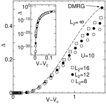
FIG. 3.: The charge gap $\Delta$ as a function of $V-V_{c}$ at $U=10$ for $L_{2}=8$, 12 and 16 together with the extrapolated result (dashed line). The solid diamond is the DMRG result [18]. Inset shows the semi-log plot of $\Delta$ near the MIT.

In Fig. 3, we plot the charge gap $\Delta$ as a function of $V-V_{c}$ at $U=10$ for $L_{2}=8$, 12 and 16 together with the result of an extrapolation with $L_{2}\to\infty$. Here, $V_{c}$ is the critical value of the MIT and determined by the condition $K_{\rho}(\ell\to\infty)=1/4$. The values of $V_{c}$ are given by 2.684, 2.583 and 2.567 for finite size systems with $L_{2}=$8, 12 and 16, respectively, which yield an $L_{2}\to\infty$ extrapolated value $V_{c}=2.55$. We note that detailed analyses of $V_{c}$ and the MIT have been already discussed in the previous works [6, 7, 8, 15, 16, 17]. The $L_{2}$-dependence of $\Delta$ is assumed to be proportional to $1/L_{2}$, resulting in an extrapolated value of $\Delta$ with $L_{2}\to\infty$ as shown in Fig. 3. The obtained result of $\Delta$ is in good agreement with the recent DMRG result of $\Delta$ at $V-V_{c}\simeq 1.45$ [18]. The inset in Fig. 3 shows the semi-log plot of $\Delta$ near the MIT. The system size dependence of $\Delta$ is very small even in the critical regime of the MIT near $V_{c}$. These results show that the new combined approach is especially efficient to analyze the very small charge gap near the MIT.

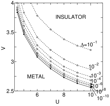
FIG. 4.: The contour lines of the charge gap $\Delta$ near the MIT on the $U$-$V$ plane. The solid line represents the phase boundary of the MIT.

In Fig. 4, we show the detailed results of contour lines for the extrapolated value of the charge gap $\Delta$ near the MIT on the $U$-$V$ plane. Rough estimation of $\Delta$ has been already reported in our previous paper [9]. However, the previous result was limited in the case with large gap ($\Delta>0.25$) region, since the usual finite size scaling is used for the ED result. We stress that our new combined approach has an ability to estimate the very small charge gap of order of $10^{-10}$ far from the limitation of the usual numerical estimation.

In summary, we examined the new combined approach of the ED, the RG and BA methods to clarify the charge gap $\Delta$ of the 1D extended Hubbard model with the on-site and the nearest-neighbor interactions $U$ and $V$ at quarter filling. Analyzing the solution of the RG equations, we connect the original system with a finite $U$ to the reference system with $U=\infty$ in which the charge gap has obtained as a function of $V$ by using the exact BA method. Adjusting the parameter $V$ of the reference system so as to fit the RG flow of the reference system to that of the original system, we estimate the absolute value of $\Delta$ of the original system including the prefactor. This approach is able to supply us with unambiguous and accurate result of $\Delta$ beyond the usual RG method and/or the ED method, even if energy scale becomes exponentially small. Detailed Analysis of $\Delta$ is shown as the contour lines on the $U$-$V$ plane in the critical regime near the MIT with very small gap.

- [1] V. J. Emery, in Highly Conducting One-Dimensional Solids, edited by J. T. Devreese, R. Evrand and V. van Doren, (Plenum, New York, 1979), p.327.
- [2] J. Sólyom, Adv. Phys. 28, 201 (1979).
- [3] For a review, J. Voit, Rep. Prog. Phys. 58, 977 (1995) and references therein..
- [4] V. J. Emery and C. Noguera, Phys. Rev. Lett. 60, 631 (1988).
- [5] K. Okamoto and K. Nomura, Phys. Lett. A169,433 (1992).
- [6] M. Nakamura, Phys. Rev. B 61, 16377 (2000).
- [7] K. Sano and Y. Ōno, J. Phys. Chem. Solids. 62, 281 (2001).
- [8] K. Sano and Y. Ōno, J. Phys. Chem. Solids. 63, 1567 (2002).
- [9] K. Sano and Y. Ōno, Phys. Rev. B70, 155102 (2004).
- [10] C. N. Yang and C. P. Yang, Phys. Rev. 151, 258 (1966).
- [11] A. Luther and Peschel, Phys. Rev. B 9, 2911 (1974).
- [12] C. N. Yang and C. P. Yang, Phys. Rev. 150, 321 (1966).
- [13] S. Kehrein, Phys. Rev. Lett. 83, 4914 (1999).
- [14] S. Kehrein, Nucl.Phys. B592, 512 (2001).
- [15] K. Penc and F. Mila, Phys. Rev. B 49, 9670 (1994).
- [16] F. Mila and X. Zotos, Europhys. Lett. 24, 133 (1993).
- [17] K. Sano and Y. Ōno, J. Phys. Soc. Jpn. 63, 1250 (1994).
- [18] S. Ejima, F. Gebhard, S. Nishimoto and Y. Ohta Phys. Rev. B 72, 33101 (2005).