Dispersionless transport in a washboard potential

Abstract

We study and characterize a new dynamical regime of underdamped particles in a tilted washboard potential. We find that for small friction in a finite range of forces the particles move essentially nondispersively, that is, coherently, over long intervals of time. The associated distribution of the particle positions moves at an essentially constant velocity and is far from Gaussian-like. This new regime is complementary to, and entirely different from, well-known nonlinear response and large dispersion regimes observed for other values of the external force.

Particle transport and diffusion in periodic potentials at finite temperatures has been addressed in so many contexts and over so many decades that one might think this to be a fully solved problem risken . However, as modern experimental and numerical methods continually evolve, ever broader parameter regimes and time regimes become accessible to inquiry, and behaviors continue to be revealed that have not previously been explored or even noted marchesoni ; reimann ; heinsalu ; hayashi ; tatarkova ; coffey ; machura ; njp ; we . Intermediate time regimes are especially challenging. On the one hand, numerical methods need to be efficient to reach beyond relatively short time behavior. On the other, analytic methods usually deal with asymptotia. Yet, experiments often involve intermediate time regimes. In this Letter we report an unexplored dynamical regime, namely, particle transport that is essentially nondispersive or coherent over long time intervals.

Consider a particle moving in a periodic potential $V(x)$ of amplitude $V_{0}$ and period $\lambda$, with coefficient of friction $\eta$ at temperature $T$, and subject to a constant external force $f$. The variables $x$ and $t$ respectively denote the position of the particle and the time. The equation of motion reads

$$\ddot{r}=-{\cal{V}}^{\prime}(r)-\gamma\dot{r}+F+\zeta(\tau),$$ (1)

where $r=x/\lambda$, $\tau=(V_{0}/m)^{1/2}t/\lambda$, the dot and prime denote derivatives with respect to $\tau$ and $r$ respectively, ${\cal{V}}(r)=V(x)/V_{0}$, and the noise obeys the fluctuation-dissipation relation $\langle\zeta(\tau)\zeta(\tau^{\prime})\rangle=2\gamma{\mathcal{T}}\delta(\tau-\tau^{\prime})$. Equation (1) models the translational Brownian motion of a particle in a tilted periodic potential, and also the rotational Brownian motion of a damped pendulum driven by a constant torque. The pendulum provides the mathematical background underlying a number of applications, including mobility in superionic conductors, dynamics of charge-density waves, ring laser gyroscopes, and phase-locking phenomena in radio engineering. Perhaps most directly relevant for experimental testing, it also models a resistively and capacitively shunted single Josephson junction. This latter correspondence has been invoked in some of the most recent work on transport in tilted periodic potentials coffey ; machura . An excellent table indicating the precise translation between the parameters of a number of physical systems including the quintessential Josephson junction testbed and our model equation can be found in coffey .

There are three independent parameters in the model, the scaled force $F=\lambda f/V_{0}$, the scaled temperature ${\cal T}=k_{B}T/V_{0}$, and the scaled dissipation $\gamma=\eta\lambda/(mV_{0})^{1/2}$. In our subsequent numerical simulations we choose ${\cal V}(r)=-(1/2)\cos(2\pi r)$, $\gamma=0.04$, and ${\mathcal{T}}=0.2$.

The external force $F$ (which we choose positive) tilts the potential, ${\cal V}(r)-Fr$. For small forces, the tilted potential has wells and barriers (“washboard potential”). Beyond a critical force $F_{c}=\pi$ the maxima and minima disappear, and the potential decreases monotonically with increasing $r$. For small $F$ the motion of a particle is essentially confined to the potential wells from which a thermal fluctuation occasionally causes it to emerge. The velocity and dispersion of the particles in this “locked state” can be understood from well-known Kramers arguments. On the other hand, when $F>F_{c}$, the periodic portion of the potential becomes unimportant; the particles follow the force with an average velocity that approaches $v=F/\gamma$ with increasing force, with a dispersion given by the Einstein law of diffusion. This is the “running state.” When the force is not too low but still well below $F_{c}$, there is a regime where particles readily alternate between the locked and running states. As a result, the mean velocity of the particles rises rapidly with increasing force, the mobility exhibits a peak associated with this rapid rise, and the dispersion also exhibits a peak that reflects the bimodal distribution of velocities risken ; njp . These well-known behaviors for underdamped particles are illustrated in Fig. 1, where we show the asymptotic mean velocity $v=\lim_{\tau\to\infty}\langle r(\tau)\rangle/\tau$ of the particles as a function of $F$, and the associated mobility $\mu=dv/dF$. In the inset we display the diffusion coefficient $D=\lim_{\tau\to\infty}\langle\Delta r^{2}(\tau)\rangle/2\tau$, where $\langle\Delta r^{2}(\tau)\rangle=\langle[r(\tau)-\langle r(\tau)\rangle]^{2}\rangle$ is the relative mean square displacement or dispersion.

Figure 1: Mean velocity $v$ (left axis, open circles) and mobility $\mu$ (right axis, black circles) vs the external force. Inset: diffusion coefficient $D$ vs external force. The “empty” portion of the diffusion coefficient curve indicates that we did not achieve a stationary state up to the longest simulation times ($\tau\sim O(10^{7})$). This is the regime of persistent dispersionless transport (see text).

The mobility and diffusion coefficient peak at a $\gamma$-dependent force more than an order of magnitude below $F_{c}$ for $\gamma=0.04$. Beyond the peaking force, the mobility reaches a constant close to $1/\gamma$. The mean velocity rises quickly as particles emerge from the well, and settles to its steady state value in times of $O(10^{2}-10^{3})$ (explicitly estimated later) for our parameters.

The as yet unexplored behavior occurs for forces above those of the mobility and diffusion peaks but below the critical force. In this regime, which extends from well below up to nearly $F_{c}$, we have exhibited no values for $D$ in the inset of Fig. 1. This is because for times that are as long as we are able to reasonably run our simulations ($\tau\sim 10^{7}$), $\langle\Delta r^{2}\rangle$ has not yet reached a behavior proportional to time. For this wide range of intermediate forces $\langle\Delta r^{2}\rangle$ remains essentially constant over time intervals that can extend over several decades, i.e., the transport is seemingly dispersionless. This coherent behavior occurs only in the underdamped system and requires there to be a washboard potential. The nondispersive behavior is remarkable because it occurs in the presence of thermal fluctuations. At sufficiently long times $\langle\Delta r^{2}\rangle$ begins to grow linearly in time, presumably also for those cases in which we were not able to reach this regime.

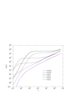
Figure 2: Dispersion vs time for different forces. Note that the curves for small ($F=0.04$) and large ($F=4.0$) forces quickly cross over from the short-time superdiffusive regime typical of low friction to the asymptotic diffusive regime. Intermediate forces exhibit a long dispersionless regime, eventually followed by normal dispersion.

Figure 2 shows the dispersion for different values of the force. For very small forces (including zero force), and also for very large forces, $\langle\Delta r^{2}\rangle$ settles into the expected linear growth with time on the same time scale as the mean velocity. The corresponding diffusion coefficients as reflected in the linear growth slopes are those shown in the inset of Fig. 1. In Fig. 2 we show two forces ($F=2.2$ and $2.5$) which exhibit the full range of behaviors of the dispersion from early rise to dispersionless regime followed by normal Einstein behavior. We also show an example of a force, $F=0.5$, for which the dispersionless regime extends over almost the entire time range of the figure after the initial rise.

Figure 3: Unnormalized distribution of particle positions at different times for $F=0.12$. Top left: early times regime. Values of $\tau$: $500$ (dot-dashed); $1000$ (solid); $2000$ (dotted); $4000$ (dashed). Bottom left: dispersionless time regime for $\tau=7000$ (solid), $30,000$ (dotted). Top right: long-time dispersive regime for $\tau=2\times 10^{5}$ (solid), $10^{6}$ (dotted). Bottom right: Log plot of bottom left distribution to display the exponential tail. The straight line is the exponential form (2) with $l_{0}=(F/\gamma)\tau_{0}=3600$.

To explore the nondispersive behavior in more detail, in Fig 3 we display simulation results for the distribution of the moving particles. Initially all the particles are placed at the minimum of one potential well, with a Maxwell-Boltzmann distribution of velocities at temperature ${\mathcal{T}}$. At early times (upper left panel) the distribution has a large peak around the origin because most of the particles are still in the initial well. As time proceeds, particles leave the well, giving rise to the second peak. The growing dispersion in this regime is due to the bimodal distribution. The maximum of the second peak moves practically from the very beginning with velocity $v\approx F/\gamma$. In time, the first peak disappears and the second peak settles into the behavior shown in the lower panels, which display the remarkable intermediate-time nondispersive behavior. The distribution of positions is a one-sided exponential that moves coherently without distortion or dispersion over a long time interval. This is particularly remarkable since during all this time (as well as before and after) the particles are persistently subject to thermal fluctuations. At sufficiently long times, dispersion resumes and the distribution not only broadens but approaches the characteristic equilibrium Gaussian shape (upper right panel). We have ascertained this same behavior for other forces. We proceed to identify the physical mechanism and to estimate the forces and crossover times for the occurrence of the dispersionless behavior.

Initially all the particles are placed in one potential well, from which they emerge according to the well-known exponential distribution of first exit times $\tau_{e}$, $P(\tau_{e})=\tau_{0}^{-1}\exp(-\tau_{e}/\tau_{0})$ redner . The mean exit time $\tau_{0}$ depends on the system parameters, the temperature, and the external force. Since the particles emerge with velocities very narrowly distributed about $v\approx F/\gamma$, this temporal distribution can be transformed to a spatial distribution of particles at $\tau=0$, $p(l_{e},0)=l_{0}^{-1}\exp(l_{e}/l_{0}),~{}{-\infty}<l_{e}\leq 0$, via the change of variables $l_{e}=(F/\gamma)\tau_{e}$. Here $l_{0}\equiv l_{\tau_{0}}\equiv(F/\gamma)\tau_{0}$. This distribution looks precisely like the ones in the lower panels of Fig. 3. At time $\tau$ the distribution will have moved to the right pretty much undistorted,

$$p(l_{e},\tau)=\frac{1}{l_{0}}\exp\left(\frac{l_{e}-l_{\tau}}{l_{0}}\right),\qquad l_{\tau}\equiv(F/\gamma)\tau.$$ (2)

The moments of this distribution are consistent with the numerical results. In particular, when $l_{\tau}\gg l_{0}$ the first moment $\to l_{\tau}$. The dispersion settles to the constant value $l_{0}^{2}$. These results reproduce the intermediate time behaviors highlighted in the simulation results.

The parameter $\tau_{0}$ defines the crossover time from short to intermediate time behavior. Its value can be extracted from the simulation results. We find $\tau_{0}=1200~{}(F=0.12)$, $490~{}(F=0.5)$, $17~{}(F=2.2)$, $3.8~{}(F=2.5)$. A theoretical estimate follows from the well-known result for the escape time of an underdamped particle from a potential well melnikov ; hanggi ; nosotros , $\tau_{0}\propto({\mathcal{T}}/\gamma U)\exp{U/{\mathcal{T}}}$. The proportionality factor varies depending on the precise definition of $\tau_{0}$, but is generally of $O(1)$. For small $F$, $U=1-F/2+O(F^{2})$; for larger $F$, $U$ is determined from a transcendental equation. This estimate leads to results consistent with the simulation values.

What marks the existence and termination of the dispersionless transport regime? There are two contributions to the width of $p(l_{e},\tau)$. One is the width $l_{0}$ due to dispersion of emergence times from the potential well, and the other comes from the thermal fluctuations. The total square width of the distribution is obtained from a convolution of these two contributions and is thus simply their sum, $\langle\Delta r^{2}(\tau)\rangle=l_{0}^{2}+2D\tau$. We stress that $D$ is the actual diffusion coefficient, which is in general different from ${\mathcal{T}/\gamma}$ (see inset in Fig. 1). The effects of the thermal fluctuations are therefore submerged until times $\tau\sim l_{0}^{2}/2D$. This estimate leads to the dispersionless ending times $\tau=5.4\times 10^{6}$ ($F=0.12$), $8.9\times 10^{4}$ ($F=2.2$), and $5.6\times 10^{3}$ ($F=2.5$), consistent with the results in Fig. 2. The seemingly anomalous dispersionless behavior is thus a natural consequence of the motion of an underdamped particle in a washboard potential.

A necessary condition for nondispersive motion is that the motion of a single particle be nonchaotic in the absence of noise. An upper bound on the forces that lead to nondispersive motion is $F=F_{c}$. A lower bound can be estimated from Fig. 1 as the force above which $v\approx F/\gamma$, which for $\gamma=0.04$ is around $F\sim 0.1$. To estimate this bound analytically and, more generally, to analyze the behavior of single particle trajectories through the dispersionless and into the dispersive regimes, we define the auxiliary variable $z(\tau)$ that describes the deviations of the particle trajectory from the approximate mean trajectory, $z=r-[l_{\tau}-l_{e}]$. The distance $l_{e}$ quickly becomes negligible. The equation of evolution for $z(\tau)$ is $\ddot{z}=-\pi\sin 2\pi(z+l_{\tau})-\gamma\dot{z}+\zeta(\tau)$, which describes a particle moving in a cosinusoidal potential that is itself rapidly and periodically oscillating in time. In the absence of noise, suppose that this particle is near the bottom of a well, slowly relaxing toward the minimum. At a time $\gamma/2F$ later it finds itself near the top of the potential, from which the small damping slowly pulls it toward the nearest minimum (either the same it was in or an adjacent one, depending on its precise location). Before it has gone far the particle again finds itself near the minimum of the well as the potential flips, the very same minimum in which it started. Again the damping pulls it toward the bottom, and the cycle restarts. The resulting $z(t)$ is thus expected to remain very small. An approximate solution for small displacements in the absence of the noise is easily obtained by approximating the nonlinear problem as a dichotomous succession of linearized problems, $\ddot{z}=-(+)2\pi^{2}z-\gamma\dot{z}$ for $\tau_{2n}<\tau<\tau_{2n+1}$ ($\tau_{2n+1}<\tau<\tau_{2n+2}$), where $\tau_{n}\equiv nF/2\gamma$ and $n=0,1,2,\cdots$. The solution of the two equations is straightforward, particularly at times $t_{2n}$,

$$z(t_{2n})=ae^{(-n\gamma^{2}/2F)}\cos\left(\theta+n\arctan\frac{\sqrt{1-A^{2}}}{A}\right),$$ (3)

where $A\equiv\cosh u\cos u$, $u=\pi\gamma/\sqrt{2}F$, $z(0)=a\cos\theta$, and we have retained only leading contributions in $\gamma/F$. The switching thus leads to a decay of solutions down to zero, which is the stabilizing behavior that leads to dispersionless motion. The solution (3) holds when $A^{2}<1$, which places the constraint $F>1.2\gamma$ on the parameters. For the value $\gamma=0.04$ used in our simulations, $F>0.05$, in gratifying agreement with the lowest forces found to lead to dispersionless transport.

Figure 4: Bottom panel: Two individual $z$-trajectories for $F=0.12$. The two trajectories emerge from the initial potential well at slightly different times of order $10^{3}$ and move essentially nondispersively for a long time, until dispersive motion eventually sets in. Upper panel: associated dispersion curve.

A clear manifestation of this description can be seen in Fig. 4. We show two individual $z$-trajectories that emerge from the potential well at different times. The associated particle trajectories are therefore in different portions of the exponential distribution of Fig. 3. The remarkable point is the flat $z$-trajectory seen in each case in the time interval between its emergence from the well to around $\tau\gtrsim 10^{5}$. This is the regime of dispersionless motion, as seen in the associated dispersion curve in the upper panel.

These arguments do not include the effects of noise, which buffets $z$ and eventually causes it to increase beyond the validity of our linearized theory. The system then no longer finds itself near the top and bottom of the flip-flopping potential but rather is sufficiently out of phase with the extrema so that the alternation does not repeatedly drive it back to the same minimum. Dispersion then sets in. Figure 4 confirms that the dispersionless motion comes to an end, and noisy motion associated with linear growth of $\langle\Delta r^{2}\rangle$ with time resumes.

In conclusion, we have identified and characterized a transport regime in the motion of thermally agitated classical particles that involves essentially dispersionless motion over several decades of time in appropriate parameter regimes. This remarkably coherent behavior requires the presence of thermal fluctuations, and is restricted to underdamped systems in a washboard potential. We have provided a theoretical framework to estimate the times of onset and duration of dispersionless transport and the parameter regimes in which it occurs. Eventually, dispersive motion sets in again and the system resumes the familiar behavior, but it may take an inordinately long time to do so, so long that it lies beyond our computational means. We are confident that the results obtained here are amenable to experimental verification. Apart from the possibility of a mechanical or electronic realization of a tilted washboard system, the regime might be observed in Josephson junctions, where the voltage (the observable) is proportional to the time derivative of the phase (corresponding to the particle coordinate in our model). It is important to note that we have also observed nondispersive behavior in numerical simulations in two dimensions with a separable potential of the form ${\cal V}(r_{x},r_{y})=-(1/2)[\cos(2\pi r_{x})+\cos(2\pi r_{y})]$. This suggests that our results may be testable on the motion of molecules and clusters on surfaces [see references in we ]. These observations give us reason to expect that this coherent dispersionless behavior should be experimentally accessible.

This work was partially supported by the National Science Foundation under Grant No. PHY-0354937 (KL), by the MCyT (Spain) under project FIS2006-11452 (JMS and AML), and by the HPC-Europa Transnational Access Program (IMS).

References

- (1) H. Risken, The Fokker-Planck Equation (Springer Verlag,New York, 1989), Ch. 11.
- (2) F. Marchesoni, Phys. Lett. A 231, 61 (1997); G. Costantini and F. Marchesoni, Europhys. Lett. 48, 491 (1999); M. Borromeo and F. Marchesoni, Surf. Sci. 465, L771 (2000).
- (3) P. Reimann et al., Phys. Rev. Lett. 87, 010602 (2001); P. Reimann et al., Phys. Rev. E 65, 031104 (2002).
- (4) E. Heinsalu, R. Tammelo, and T. Örg, Phys. Rev E 69, 021111 (2004).
- (5) K. Hayashi and S. Sas, Phys. Rev. E 69, 066119 (2004).
- (6) S. A. Tatarkova, W. Sibbett, and K. Dholakia, Phys. Rev. Lett. 91, 038101 (2003).
- (7) W. T. Coffey, Yu. P. Kalmykov, S. V. Titov, and B. P. Mulligan, Phys. Rev. e 73, 061101 (2006).
- (8) L. Machura, M. Kostur, P. Talkner, J. Luczka, and P. Hänggi, cond-mat/0609452.
- (9) K. Lindenberg, A. M. Lacasta, J. M. Sancho, and A. H. Romero, New J. Phys. 7, 29 (2005).
- (10) J. M. Sancho, A. M. Lacasta, K. Lindenberg, I. M. Sokolov, and A. H. Romero, Phys. Rev. Lett. 92, 250601 (2004); A. M. Lacasta, J. M. Sancho, A. H. Romero, I. M. Sokolov, and K. Lindenberg, Phys. Rev. E 70, 051104 (2004).
- (11) S. Redner, A Guide to First-Passage Processes (Cambridge University Press, 2001).
- (12) V. I. Melnikov and S. V. Meshkov, J. Chem. Phys. 91, 4073 (1986); V. I. Melnikov, Phys. Rep. 209, 1 (1991).
- (13) P. Hänggi, P. Talkner, and M. Borkovec, Rev. Mod. Phys. 62, 251 (1990).
- (14) J. M. Sancho, A. H. Romero, and K. Lindenberg, J. Chem. Phys. 109, 9888 (1998).