Nonequilibrium thermal entanglement

Abstract

Results on heat current, entropy production rate and entanglement are reported for a quantum system coupled to two different temperature heat reservoirs. By applying a temperature gradient, different quantum states can be found with exactly the same amount of entanglement but different purity degrees and heat currents. Furthermore, a nonequilibrium enhancement-suppression transition behavior of the entanglement is identified.

I I. Introduction

Quantum thermodynamics rego ; mahler is starting to throw light on universal behaviors of nanosystems. Specifically, new possibilities arising in nonequilibrium situations, with dominant quantum coherences, are emerging scully . Currently, non-local quantum correlations (entanglement) are being considered in a vast variety of scenarios as they are key ingredients for novel and non-conventional forms of communication, information processing and computation. For potential large-scale applications, where condensed matter systems are of prime importance, thermal interactions with specific environments are unavoidable. Thus a clear connection between quantum information aspects and thermal magnitudes has to be elucidated. Furthermore, the biological frontier of physics imposes to address the question of quantum features survival in noisy as well as in nonequilibrium conditions phillips .

For quantum systems in contact with heat reservoirs at unique and fixed temperature, the equilibrium thermal entanglement has been extensively studied vedral ; wang ; kamta ; canosa . Until now, most of the emphasis in the study of thermal entanglement has been confined to equilibrium situations. Entanglement in nonequilibrium quantum systems has been scarcely considered and thus a proper description of thermal entanglement in the presence of matter and/or energy currents is still lacking. Recently, Eisler et al. eisler has calculated the Von Neumann entropy of a block of spins in a XX spin chain in the presence of an energy current, showing that an enhancement of the amount of entanglement due to an energy current is possible. The energy current is modelled by adding an extra term to the spin chain Hamiltonian for simulating a steady-state current in a thermodynamic closed system. However, the issue of entanglement behavior in true nonequilibrium conditions of a thermodynamic open system remains untouched.

Two coupled qubits in thermal contact with different heat baths is a system not only of theoretical interest but a common place in nanophysics. In semiconductor quantum dots the transfer of quantum information between nuclear spins and electronic spins has been recently considered quiroga ; imamoglu1 ; loss . The nuclear spin is generally weakly coupled to its environment while the electronic spin is strongly coupled to a great variety of degrees of freedom within the solid. In this way, the effective environments are different for both kind of spins. Besides that, nuclear magnetic resonance techniques allow the cooling of nuclear spins in a controlled manner imamoglu2 ; lai without significatively affecting the electronic spins, thus creating two reservoirs at effective different temperatures. On the other hand, superconductor qubits can be easily designed to be coupled to different environments. For instance, inductively coupled superconductor flux qubits in contact with two different environments has been recently analyzed in Ref.storcz . The aim of the present paper is to correlate thermodynamical nonequilibrium steady-state features with entanglement properties of quantum nanosystems. In doing so, we shall consider a quantum system in a nonequilibrium condition for which the amount of entanglement can be exactly evaluated: two interacting qubits (spins) in contact with two heat reservoirs at different temperatures. In this case, entanglement can be evaluated for any mixed state by using the concurrence wooters . Indeed, the model system to be considered in the present work should be useful for a large variety of physical set ups aiming to explore the relationship between quantum informational entropy and thermodynamic entropy at the atomic scale. Whether one can reveal universal features in irreversible processes of open quantum systems is of great significance.

II II. Formalism

The central quantum nanosystem is described by a Hamiltonian $\hat{Q}$, interacting with two heat reservoirs which are assumed to be in a permanent thermodynamical equilibrium at $\beta_{i}=1/k_{B}T_{i},i=1,2$ ($k_{B}=\hbar=1$) with internal Hamiltonians $\hat{R}_{i}$. The total Hamiltonian is then

$$\hat{H}=\hat{Q}+\hat{R}_{1}+\hat{R}_{2}+\hat{S}_{1}+\hat{S}_{2}$$ (1)

where the nanosystem is simultaneously coupled with both reservoirs through terms $\hat{S}_{1}$ y $\hat{S}_{2}$. The nanosystem + reservoirs is described by a density operator satisfying the Liouville equation $\frac{d\hat{\gamma}}{dt}=-i[\hat{H},\hat{\gamma}]$. We assume that the coupling strengths of the central quantum system to the reservoirs are weak so that the full density operator $\hat{\gamma}$ can be expressed as $\hat{\gamma}(t)=\hat{\rho}(t)\hat{\rho}_{1}\hat{\rho}_{2}$ where each reservoir is described by its own canonical equilibrium density operator $\hat{\rho}_{i}=e^{-\beta_{i}\hat{R}_{i}}/Tr_{R_{i}}\{e^{-\beta_{i}\hat{R}_{i}}\}\}$ and $\hat{\rho}(t)$ is the reduced density operator for the quantum system of interest. The couplings nanosystem-reservoirs are written as

$$\hat{S}_{1}+\hat{S}_{2}=\sum_{j=1}^{2}\sum_{\mu}\hat{V}_{j,\mu}\hat{f}_{j,\mu}=\sum_{j=1}^{2}\sum_{\mu}\hat{V}^{{\dagger}}_{j,\mu}\hat{f}^{{\dagger}}_{j,\mu}$$ (2)

where the nanosystem operators $\hat{V}_{j,\mu}$ are taken to satisfy $[\hat{Q},\hat{V}_{j,\mu}]=\omega_{j,\mu}\hat{V}_{j,\mu}$ and the operators $\hat{f}_{j,\mu}$ act on the reservoir degrees of freedom ($j=1,2$). Within the framework of the Born-Markov approximation goldman , the equation of motion for $\hat{\rho}(t)$ is given by

$$\frac{d\hat{\rho}}{dt}=-i[\hat{Q},\hat{\rho}(t)]-\sum_{j=1}^{2}\sum_{\mu,\nu}J_{\mu,\nu}^{(j)}(\omega_{j,\nu})$$

$$\{[\hat{V}_{j,\mu},[\hat{V}^{{\dagger}}_{j,\nu},\hat{\rho}]]-(1-e^{\beta_{j}\omega_{j,\nu}})[\hat{V}_{j,\mu},\hat{V}^{{\dagger}}_{j,\nu}\hat{\rho}]\}$$ (3)

where the spectral density of the $j$-th reservoir is

$$J_{\mu,\nu}^{(j)}(\omega_{j,\nu})=\int_{0}^{\infty}d\tau e^{i\omega_{j,\nu}\tau}Tr_{R_{j}}\{\hat{\rho}_{j}\bar{f}^{{\dagger}}_{j,\nu}(\tau)\hat{f}_{j,\mu}\}$$ (4)

with $\bar{f}^{{\dagger}}_{k,\nu}(\tau)=e^{-i\hat{R}_{k}\tau}\hat{f}^{{\dagger}}_{k,\nu}e^{i\hat{R}_{k}\tau}$.

We will here be concerned with the simplest possible scenario where clear relations between informational and thermodynamic entropies could be found. To set up our model system in a general context, we consider a nanosystem composed of two interacting qubits as described by the Hamiltonian

$$\hat{Q}=\sum_{\alpha=1}^{2}\frac{\epsilon_{\alpha}}{2}\hat{\sigma}_{\alpha,z}+K(\hat{\sigma}_{1}^{+}\hat{\sigma}_{2}^{-}+\hat{\sigma}_{1}^{-}\hat{\sigma}_{2}^{+})+K^{\prime}\hat{\sigma}_{1,z}\hat{\sigma}_{2,z}$$ (5)

where $\hat{\sigma}_{\alpha,z}$ and $\hat{\sigma}_{\alpha}^{\pm}$ denote Pauli matrices. The inter-qubit coupling is ferromagnetic when $K,K^{\prime}<0$ and antiferromagnetic when $K,K^{\prime}>0$. This type of Hamiltonian encompasses three well-known spin models: it turns into the isotropic Heisenberg-like coupling for $K=K^{\prime}$, the isotropic XX-like model for $K^{\prime}=0$ and the Ising-like model for $K=0$. The eigenenergies and eigenstates corresponding to Eq.(5) are: $|s_{1}\rangle=|0,0\rangle$ ($E_{1}=-\frac{\epsilon_{1}+\epsilon_{2}}{2}+K^{\prime}$), $|s_{2}\rangle=|1,1\rangle$ ($E_{2}=\frac{\epsilon_{1}+\epsilon_{2}}{2}+K^{\prime}$), $|s_{3}\rangle={\rm cos}(\theta/2)|1,0\rangle+{\rm sin}(\theta/2)|0,1\rangle$ ($E_{3}=\alpha-K^{\prime}$) and $|s_{4}\rangle=-{\rm sin}(\theta/2)|1,0\rangle+{\rm cos}(\theta/2)|0,1\rangle$ ($E_{4}=-\alpha-K^{\prime}$), with $\alpha=\sqrt{K^{2}+\frac{(\epsilon_{1}-\epsilon_{2})^{2}}{4}}$ and ${\rm tan}\theta=2K/(\epsilon_{1}-\epsilon_{2})$. We consider each qubit in contact with its own boson heat reservoir through a term of the form

$$\hat{S}_{j}=\hat{\sigma}_{j}^{+}\sum_{n}g^{(j)}_{n}\hat{a}_{n,j}+\hat{\sigma}_{j}^{-}\sum_{n}g^{(j)*}_{n}\hat{a}^{{\dagger}}_{n,j}\quad,\quad j=1,2$$ (6)

where $\hat{a}^{{\dagger}}_{n,j}$ creates an excitation in mode $n$ of reservoir $j$ with a coupling strength $g^{(j)}_{n}$.

The nonequilibrium steady-state density matrix (designed simply as $\hat{\rho}$ from now on), must satisfy $\frac{d\hat{\rho}}{dt}=-i[\hat{Q},\hat{\rho}]=0$ in Eq.(3), which yields to ${\cal L}_{1}(\hat{\rho})+{\cal L}_{2}(\hat{\rho})=0$ where the Lindblad or relaxation super-operators are given by

$${\cal L}_{j}(\hat{\rho})= - \sum_{\mu=1}^{4}J^{(j)}(\omega_{\mu})\{-\hat{V}_{j,\mu}\hat{\rho}\hat{V}^{{\dagger}}_{j,\mu}+\hat{\rho}\hat{V}^{{\dagger}}_{j,\mu}\hat{V}_{j,\mu}+e^{\beta_{j}\omega_{\mu}}(\hat{V}_{j,\mu}\hat{V}^{{\dagger}}_{j,\mu}\hat{\rho}-\hat{V}^{{\dagger}}_{j,\mu}\hat{\rho}\hat{V}_{j,\mu})\}$$ (7)

$$- \sum_{\mu=1}^{4}J^{(j)}(-\omega_{\mu})\{-\hat{V}^{{\dagger}}_{j,\mu}\hat{\rho}\hat{V}_{j,\mu}+\hat{\rho}\hat{V}_{j,\mu}\hat{V}^{{\dagger}}_{j,\mu}+e^{-\beta_{j}\omega_{\mu}}(\hat{V}^{{\dagger}}_{j,\mu}\hat{V}_{j,\mu}\hat{\rho}-\hat{V}_{j,\mu}\hat{\rho}\hat{V}^{{\dagger}}_{j,\mu})\}$$

for $j=1,2$. In the latter expression $\omega_{1}=E_{2}-E_{3},\hat{V}_{j,1}=(\delta_{j,2}{\rm cos}(\theta/2)+\delta_{j,1}{\rm sin}(\theta/2))|s_{2}\rangle\langle s_{3}|$; $\omega_{2}=E_{2}-E_{4},\hat{V}_{j,2}=(-\delta_{j,2}{\rm sin}(\theta/2)+\delta_{j,1}{\rm cos}(\theta/2))|s_{2}\rangle\langle s_{4}|$; $\omega_{3}=E_{3}-E_{1},\hat{V}_{j,3}=(\delta_{j,1}{\rm cos}(\theta/2)+\delta_{j,2}{\rm sin}(\theta/2))|s_{3}\rangle\langle s_{1}|$; $\omega_{4}=E_{4}-E_{1},\hat{V}_{j,4}=(-\delta_{j,1}{\rm sin}(\theta/2)+\delta_{j,2}{\rm cos}(\theta/2))|s_{4}\rangle\langle s_{1}|$ and $J^{(j)}(-\omega_{\mu})=e^{\beta_{j}\omega_{\mu}}J^{(j)}(\omega_{\mu})$. Two limiting cases can be easily analyzed: (i) No inter-qubit coupling, $K=K^{\prime}=0$ ($\theta=0$) which leads to $\omega_{1}=\omega_{4}=\epsilon_{2}$ and $\omega_{2}=\omega_{3}=\epsilon_{1}$. Each qubit reaches a local equilibrium with its own heat reservoir yielding to a direct product form of the density matrix and thus no-entanglement. (ii) Coupled qubits, $K,K^{\prime}\neq 0$, in contact with two independent reservoirs at identical temperatures, $\beta_{1}=\beta_{2}=\beta$. A reduced density matrix results which has the thermodynamical canonical form for a system described by internal Hamiltonian $\hat{Q}$ at equilibrium with a thermal bath at inverse temperature $\beta$, as it should be.

III III. Results and Discussion

Consistently with the Born-Markov approximation, we adopt a Weisskopf-Wigner-like expression such as $J^{(j)}(\omega_{\mu})=\Gamma_{j}(\omega_{\mu})n_{j}(\omega_{\mu})$ where $\Gamma_{j}(\omega_{\mu})$ depends on both the nanosystem-$j$th-reservoir coupling strength and the reservoir internal structure. On the other hand, $n_{j}(\omega_{\mu})=(e^{\beta_{j}\omega_{\mu}}-1)^{-1}$ denotes the thermal mean value of the number of excitations in reservoir $j$ at frequency $\omega_{\mu}$. For the sake of simplicity, we take identical and frequency independent couplings, thus $\Gamma_{1}(\omega)=\Gamma_{2}(\omega)=\Gamma$.

From Eq.(7) the nonequilibrium steady-state density matrix is obtained as given by the diagonal matrix $\hat{\rho}=diag\{\rho_{1,1},\rho_{2,2},\rho_{3,3},\rho_{4,4}\}$ in the basis of eigenstates of $\hat{Q}$. Although, it can be analytically expressed we will not go here into the details as its explicit form is cumbersome qrrp . Instead, we shall analyze some important special situations.

III.1 A. Symmetric case, $\epsilon_{1}=\epsilon_{2}=\epsilon$

In this case $\hat{\rho}$ can be written in terms of a simple universal function $e(\omega)=\frac{n_{1}(\omega)+n_{2}(\omega)}{1+n_{1}(\omega)+n_{2}(\omega)}\leq 1$ (energies and temperatures in units of interqubit coupling $K=1$). In the strong coupling case ($\epsilon<1$) we found

$$\rho_{1,1}=\frac{e_{1}}{2}\left(1-\frac{e_{2}}{2}\right) \rho_{2,2}=\left(1-\frac{e_{1}}{2}\right)\frac{e_{2}}{2}$$ ;

$$\rho_{3,3}=\frac{e_{1}}{2}\frac{e_{2}}{2} \rho_{4,4}=\left(1-\frac{e_{1}}{2}\right)\left(1-\frac{e_{2}}{2}\right)$$ ; (8)

where $e_{j}=e(\omega_{j})$ with $\omega_{1}=\omega_{4}=|\epsilon-1|$ and $\omega_{2}=\omega_{3}=\epsilon+1$. In the weak coupling case ($\epsilon>1$) the following interchanges have to be made: $\rho_{1,1}\leftrightarrow\rho_{4,4}$ and $\rho_{2,2}\leftrightarrow\rho_{3,3}$. Thus, the nonequilibrium concurrence is $C=2Max\{0,|\rho_{3,3}-\rho_{4,4}|/2-\sqrt{\rho_{1,1}\rho_{2,2}}\}$.

Let us first discuss the equilibrium ($T_{1}=T_{2}=T$) thermal entanglement behavior for a system governed by Hamiltonian (5) vedral ; wang ; kamta ; canosa . An analytical expression can be found for the equilibrium concurrence as $C_{eq}(T)=\frac{{\rm sinh}(1/T)-1}{2{\rm cosh}(\omega_{1}/2T){\rm cosh}(\omega_{2}/2T)}$. This last expression is interesting because it implies an universal form (independent of $\epsilon$) for the sudden death of the equilibrium concurrence at the temperature $T_{c}=1.1346$. For $\epsilon<1$, the two-qubit concurrence decreases from 1 to 0 as the temperature increases up to $T_{c}$; for $\epsilon>1$, the concurrence increases from 0 to some maximum before vanishing at $T_{c}$. It is also known that the concurrence decreases monotonically as the qubit splitting increases for any temperature and vanishes exponentially with increasing $\epsilon$. All these features are independent of the specific nature of the reservoirs.

The behavior of quantum states, for any qubit internal splitting and reservoir temperatures, can be displayed in a single plot $e_{1}$-$e_{2}$, as it is shown in Fig. 1. Although, the quantum state variation is described by the same curve for $\epsilon$ and $1/\epsilon$, the border lines separating the entangled from the unentangled regions are different: the green curve corresponds to $\epsilon<1$ while the red curve corresponds to $\epsilon>1$. The black line represents equilibrium quantum states for both $\epsilon=1/3$ as well as for $\epsilon=3$. The shifting of the quantum state with the temperature gradient, $\Delta T=T_{1}-T_{2}$, is depicted by the circles, for the same average temperature, $T_{M}=(T_{1}+T_{2})/2=1$. It is evident that the temperature gradient shifts the state from the entangled zone to the unentangled zone. However, this behavior can be reversed at low temperatures for $\epsilon>1$ as it is to be discussed below.

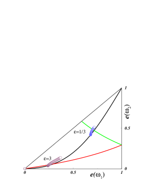
Figure 1: (Color online) Quantum state parameter space ($e_{1}$, $e_{2}$). The black line denotes equilibrium states. Green line: entangled-unentangled border for $\epsilon<1$. Red line: entangled-unentangled border for $\epsilon>1$. Circles represent the state shift under a temperature gradient from the same mean temperature $T_{M}=1$. Blue circles: $\epsilon=1/3$, brown circles: $\epsilon=3$.

In the linear nonequilibrium limit (LNEL), $\Delta T\ll 1$, the concurrence can be written as $C(\Delta T)=Max\{0,C_{eq}(T_{M})-\alpha\Delta T^{2}\}$ where the coefficient $\alpha$ is a function of the average temperature as well as the qubit internal splitting. The equilibrium concurrence is displayed in the insets of Figs. 2-a and 2-b. In the strong coupling limit ($\epsilon<1$) $\alpha>0$ thus the concurrence is always a decreasing function of the temperature gradient $\Delta T$. By contrast, in the weak coupling limit ($\epsilon>1$) there is a transition mean temperature for which $\alpha$ changes the sign. Thus, a low temperature region can be found where $\alpha<0$ for which a gradient temperature produces an increasing of the concurrence as compared with the equilibrium case. The degree of mixing of the quantum state can be characterized by the linear entropy as defined by $S_{L}=(4/3)(1-Tr\{\hat{\rho}^{2}\})$. The low $\Delta T$ limit of the linear entropy can also be expanded as $S_{L}(\Delta T)=S_{L,eq}(T_{M})+\alpha^{\prime}\Delta T^{2}+O(\Delta T^{4})$. The coefficient $\alpha^{\prime}>0$, for both interqubit coupling cases, is also illustrated in Figs. 2-a and 2-b. Note that while a temperature gradient can produce, in a limited temperature interval, an enhancement of the concurrence it always yields to a more mixed state. This result will permit to prepare a great variety of quantum states with practically any combination of entanglement and purity degree by varying the temperature of only one heat reservoir.

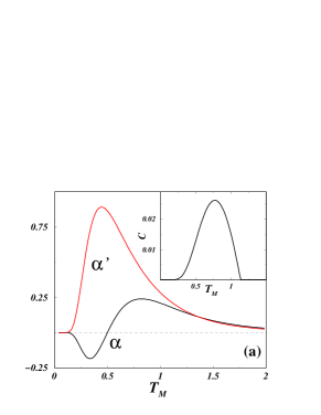
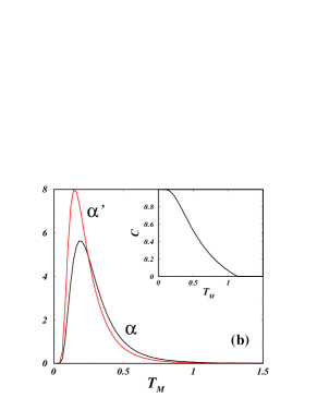
Figure 2: (Color online) LNEL coefficients $\alpha$ and $\alpha^{\prime}$, denoting the second order in $\Delta T$ variation of the concurrence and linear entropy, respectively: (a) $\epsilon=3$, (b) $\epsilon=1/3$. Insets: Equilibrium concurrence.

The relationship between a nonequilibrium thermodynamical quantity such as the heat current and a central quantum information concept such as entanglement is now addressed. We start by calculating the heat current as ${\cal J}_{j}=Tr\{\hat{Q}{\cal L}_{j}(\hat{\rho})\}$ breuer , which in the symmetric case yields to

$${\cal J}_{1} = \frac{1}{4}[\omega_{1}(1-e_{1})\left(n_{2}(\omega_{1})-n_{1}(\omega_{1})\right)-(1\leftrightarrow 2)]$$ (9)

and ${\cal J}_{2}=-{\cal J}_{1}=-{\cal J}$. In LNEL, $\Delta T\ll 1$, the Fourier’s law is well verified, i.e. ${\cal J}=\kappa\Delta T$, with $\kappa$ the thermal conductance depending on the qubit internal splitting and mean temperature qrrp . The evolution of heat current and concurrence, as $\Delta T$ increases is illustrated in Fig. 3 (obviously ${\cal J}=0$ for $\Delta T=0$). Clearly, for temperatures for which $\alpha<0$, see Fig. 2-a, an enhancement of the concurrence is possible by applying a temperature gradient. Based on this general concurrence’s behavior, we conclude that in LNEL, ${\cal J}(\Delta T)=\frac{\kappa}{\sqrt{\alpha}}|C_{eq}-C(\Delta T)|^{1/2}$ as it is clearly observed in Fig. 3. A remarkable point to be noted is the possibility of constructing nonequilibrium quantum states with identical concurrence, as that for the equilibrium case, but carrying a heat current. It is also evident from Fig. 3 that the relation between heat current and concurrence becomes independent of $T_{M}$ as the temperature gradient increases. The correlation between quantum linear entropy $S_{L}$ and concurrence is also shown in the inset of Fig. 3, confirming the fact that a gradient temperature will always increase the mixing degree of the quantum state. Although, the amount of entanglement is small in those cases, it can be significantly increased by distillation protocols.

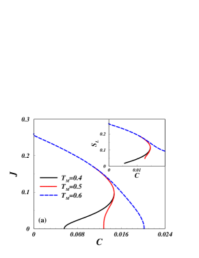
Figure 3: (Color online) Heat current ${\cal J}$ and concurrence evolution for different mean temperatures $T_{M}$. Inset: Linear entropy and concurrence. Each point corresponds to a $\Delta T$ value.

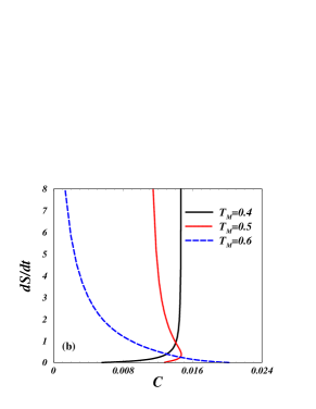
Figure 4: (Color online) Thermodynamical entropy production rate and concurrence evolutions for different mean temperatures $T_{M}$. Each point corresponds to a $\Delta T$ value.

Any heat current produces an amount of thermodynamical entropy proportional to the heat which is carried on and inversely proportional to the temperature of the reservoir from which the heat is extracted (or injected). Thus, the thermodynamic entropy production rate in our system can be written as $dS/dt={\cal J}_{1}(T_{1}^{-1}-T_{2}^{-1})$ prigogine . In LNEL, the rate of entropy production shows a linear dependence with the concurrence as $\frac{dS}{dt}=\frac{2\kappa}{\alpha T_{M}^{2}}|C_{eq}-C(\Delta T)|$ as it is shown in Fig. 4. The entropy production rate, like the heat current and linear entropy, is always different for two different values of $\Delta T$ corresponding however to the same amount of entanglement.

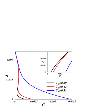
Figure 5: (Color online) Heat current ${\cal J}$ and concurrence evolution for different mean temperatures $T_{M}$ in the non-symmetric case, $\epsilon_{1}=8$ and $\epsilon_{2}=3$. Inset: $\epsilon_{1}=3$ and $\epsilon_{2}=8$. Each point corresponds to a $\Delta T$ value.

III.2 B. Non-symmetric case, $\epsilon_{1}>\epsilon_{2}$

We first consider the high temperature reservoir ($T_{1}$) is in direct contact with the large splitting qubit, $\epsilon_{1}$, and the low temperature reservoir ($T_{2}$) is in contact with the small splitting qubit, $\epsilon_{2}$. Modifications to equilibrium values of physical magnitudes such as the concurrence and the linear entropy are now of first order in $\Delta T$ instead of order $\Delta T^{2}$, as it was the case for the symmetric set up. This implies that in LNEL ${\cal J}(\Delta T)\sim|C_{eq}-C(\Delta T)|$, as is illustrated in Fig. 5. Note that at low temperature it arises the possibility of finding up to three quantum states with the same concurrence but carrying different heat currents. Switching to the inverse connection between qubits and reservoirs ($T_{1}\leftrightarrow T_{2}$), the heat current dependence on the concurrence is completely modified. In this latter case, high temperature bath in contact with the low splitting qubit, the heat current is substantially decreased but the concurrence can be enhanced by the temperature gradient, as it is shown in the inset of Fig. 5. We conclude that a qubit splitting asymmetry brings an interesting new control parameter for engineering nonequilibrium thermal quantum states.

IV IV. Conclusions

In summary, we have demonstrated that under nonequilibrium thermal conditions a versatile scenario for tailoring heat carrying quantum states with a well specified amount of entanglement is feasible. A temperature gradient has been shown to produce increasing or decreasing entanglement depending on the internal coupling strength within a nanosystem. Physical realizations of the model system we addressed are provided by a large number of physical systems such as nuclear spins in quantum dots and superconducting qubits. Therefore, the resulting insights can serve as useful recipes for realistic quantum information processors in noisy and nonequilibrium environments.

L.Q. and F.J.R. acknowledge financial support from COLCIENCIAS and Facultad de Ciencias-Uniandes-2006. M.E.R. and R. P. acknowledge financial support from Vicerrectoría Académica (2004-5), Universidad Javeriana-Bogotá.

References

- (1) L.G.C.Rego et al., Phys.Rev.Lett. 81, 232 (1998).
- (2) M.Michel et al., Phys.Rev.Lett. 95, 180602 (2005); M.Hartmann et al., ibid 93, 080402 (2004); M.J.Henrich et al., cond-mat/0604202.
- (3) M.O.Scully et al., Science 299, 862 (2003).
- (4) R.Phillips et al., Physics Today, May 2006, page 38.
- (5) D.Gunlycke et al., Phys.Rev. A64, 042302 (2001).
- (6) X.Wang, Phys.Rev. A64, 012313 (2001); ibid A66, 034302 (2002); ibid A66, 044305 (2002); X.Wang et al., Eur.Phys.J. D18, 285 (2002).
- (7) G.Lagmago Kamta et al., Phys.Rev.Lett. 88, 107901 (2002).
- (8) N.Canosa et al., Phys.Rev. A73, 022347 (2006).
- (9) V.Eisler et al., Phys.Rev. A71, 042318 (2005).
- (10) J.H.Reina et al., Phys.Rev. B62, 2267 (2000).
- (11) A.Imamoglu et al., Phys.Rev.Lett. 91, 017402 (2003).
- (12) A.Khaestkii et al., Phys.Rev. B67, 195329 (2003); W.A.Coish et al., ibid B72, 125337 (2005).
- (13) D.Stepanenko et al., Phys.Rev.Lett. 96, 136401 (2006).
- (14) C.W.Lai et al., Phys.Rev.Lett. 96, 167403 (2006).
- (15) M.J.Storcz et al., Phys.Rev. A67, 042319 (2003).
- (16) W.K.Wootters, Phys.Rev.Lett. 80, 2245 (1998).
- (17) M.Goldman, J.Magn.Reson. 149, 160 (2001).
- (18) L.Quiroga et al., to be published.
- (19) H.-P.Breuer and F.Petruccione, The Theory of Open Quantum Systems (Oxford University Press, 2002).
- (20) I.Prigogine, Introduction to Thermodynamics of Irreversible Processes, third ed. (John Wiley Sons, 1967).