Negative Entropy Production in Oscillatory Processes

Abstract

Linear irreversible thermodynamics asserts that the instantaneous local spontaneous entropy production is always nonnegative. However for a viscoelastic fluid this is not always the case. Given the fundamental status of the Second Law, this presents a problem. We provide a new derivation of the Second Law, from first principles, which is valid for the appropriately time averaged entropy production allowing the instantaneous entropy production to be negative for short intervals of time. We show that time averages (rather than instantaneous values) of the entropy production are nonnegative. We illustrate this using molecular dynamics simulations of oscillatory shear.

Linear irreversible thermodynamics asserts that in local equilibrium key-16 , the spontaneous entropy production per unit time, per unit volume, the so-called entropy source strength $\sigma(\mathbf{\mathbf{r}},t)$, cannot be negative key-1 ; key-3 . Further it states that the entropy source strength is a sum of products of irreversible thermodynamic fluxes $J_{i}$ and forces $X_{i}$,

$$\sigma(\mathbf{r},t)=\sum J_{i}(\mathbf{r},t)X_{i}(\mathbf{r},t)\geq 0$$ (1)

where the source strength is calculated at a position $\mathbf{r}$ and a time $t$. For steady state processes close to equilibrium Eq. 1 is clearly correct. However, for processes that involve time dependent or oscillatory thermodynamic forces, in viscoelastic materials close to equilibrium, Eq. 1 is incorrect. These problems are usually resolved by separating the fluxes into “storage and loss” components key-4 . Such a separation is not derived from first principles and is process specific. A second problem with Eq. 1 is that it is restricted to the near equilibrium, linear response, regime. Further from equilibrium the definition of entropy and therefore temperature remains an unsolved problem key-11 . Until very recently there has been no known generalization of Eq. 1 to the far from equilibrium regime.

Recent advances, which are of broad interest key-12 ; key-13 , have cast new light on these issues. In particular we will use the Jarzynski Equality (JE) Jarzynski PRL ; Jarzynski PRE to derive a variation on Eq. 1 from first principles. In order to proceed we first define the conjugate flux $\mathbf{J}$, for a system which is driven away from equilibrium by a dissipative field $\mathbf{F}_{e}$, in terms of the rate that work is done on the system evans-morriss ,

$$\mathbf{J}V\cdot\mathbf{F}_{e}\left(t\right)=-k_{B}T\Omega\left(t\right)\equiv k_{B}T\Lambda\left(\mathbf{\Gamma}\left(t\right)\right)-\frac{d}{dt}H_{0}\left(\mathbf{\Gamma}\left(t\right)\right).$$ (2)

Here $V$ is the system volume, $k_{B}$ is Boltzmann’s constant, $T$ is the temperature of the synthetic thermostat or a large heat reservoir williams PRE 04 , $\Omega(t)$ is the dissipation function as defined for the Evans-Searles Fluctuation Theorem evans-searles adv phys , $\mathbf{\Gamma}\left(t\right)$ is the phase space vector, $H_{0}$ is the internal energy, $k_{B}T\Lambda$ gives the rate that heat is lost from the system to the thermostat or reservoir williams PRE 04 and $\Lambda$ is the phase space compression factor evans-morriss . Eq. 2 is defined for arbitrary field strengths and in the linear response regime it gives the entropy production,

$$-\langle\mathbf{J}V\cdot\mathbf{F}_{e}\left(t\right)\rangle/T=k_{B}\left\langle\Omega(t)\right\rangle=\int_{V}d\mathbf{r}\,\sigma\left(\mathbf{r},t\right)+O\left(F_{e}^{4}\right),$$ (3)

where $\left\langle...\right\rangle$ denotes an ensemble average.

The JE has been shown Jarzynski PRL ; Jarzynski PRE and proved Evans Mol Phys 03 for the time reversible thermostatted dynamics we employ below. It has also been experimentally verified Bustamante sci ; collin nat . The JE gives the change in Helmholtz free energy $\Delta A$ for a system which has undergone a nonequilibrium process starting from an initial ($t=0$) equilibrium distribution of phases $f_{1}(\mathbf{\Gamma},0)\propto exp[-\beta H(\mathbf{\Gamma},\lambda(0))]$ and initial Hamiltonian $H(\mathbf{\Gamma},\lambda(0))$ to a final Hamiltonian $H(\mathbf{\Gamma},\lambda(\tau))$ at $t=\tau$ and then relaxed to a new equilibrium. The dynamical proof Evans Mol Phys 03 requires that the dynamical pathway $\mathbf{\Gamma}(t)$ be such that the distribution of phases at $t=\tau$ can subsequently relax to a final canonical distribution at $t=\infty$, $f_{\infty}(\mathbf{\Gamma},\infty)\propto exp[-\beta H(\mathbf{\Gamma},\lambda(\tau))]$. The parametric transformation of the Hamiltonian is complete at a finite time $t=\tau$, by which time the system is not expected to have fully relaxed to the new equilibrium. JE states,

$$\left\langle\exp\left(-\beta W_{\tau}\right)\right\rangle=\exp\left(-\beta\Delta A\right).$$ (4)

where $W_{\tau}=\int_{0}^{\tau}ds\dot{W}(s)$ is the Jarzynski work function and $\dot{W}(t)\equiv[\frac{d}{dt}H_{0}(\Gamma(t),\lambda(t))]-k_{B}T\Lambda(\mathbf{\Gamma}(t))$, Evans Mol Phys 03 . Although $H_{0}(\mathbf{\Gamma}(\tau),\lambda(\tau))\neq H_{0}(\mathbf{\Gamma}(\infty),\lambda(\tau))$ it is clear that, $W_{\tau}=W_{\infty}$.

The proof of the JE Evans Mol Phys 03 requires that the two systems be connected by a path $1\rightarrow 2$ and its inverse path $2\rightarrow 1$. The proof does not put restrictions on the time dependence of the path. The parametric change in the Hamiltonian from $\lambda(0)\rightarrow\lambda(\tau)$ may in addition contain work due to the system being driven by a dissipative external field Evans Mol Phys 03 . If the work is solely due to a dissipative external field ($\dot{\lambda}=0\;\;\forall\;\;t$) then the rate of work $\dot{W}$ will be the same as that given by Eq. 2 (ie $\dot{W}=k_{B}T\Omega$).

The JE allows a first principles proof of the Second Law Inequality (SLI) from the equations of motion as first shown by Jarzynski Jarzynski PRE . By combining Eq. 4 with the mathematical identity $\exp(x)\geqslant 1+x$ we have,

$$e^{-\beta\Delta A}=\langle e^{-\beta(W_{\tau}-\langle W_{\tau}\rangle)}\rangle e^{-\beta\langle W_{\tau}\rangle}\geq e^{-\beta\langle W_{\tau}\rangle}.$$ (5)

Noting that $e^{x}$ is a monotonically increasing function we derive the Clausius Inequality

$$\left\langle W_{\tau}\right\rangle\geq\Delta A,\>\;\forall\;\>\tau\geq 0.$$ (6)

If the system of interest is a fluid and if the transformation involves, say, a shearing deformation or perhaps the translation of one particle through a fixed distance, then clearly $\Delta A=0$, we may treat the field as external $\dot{\lambda}=0$, and thus, by Eq. 2, $W_{\tau}=k_{B}T\bar{\Omega}_{\tau}\tau=-\int_{0}^{\tau}ds\,\mathbf{J}\left(s\right)V\cdot\mathbf{F}_{e}\left(s\right)$ where $\bar{\Omega}_{\tau}\equiv\frac{1}{\tau}\int_{0}^{\tau}ds\,\Omega(s)$. The SLI then follows,

$$\left\langle\bar{\Omega}_{\tau}\right\rangle=-\frac{1}{\tau k_{B}T}\int_{0}^{\tau}ds\,\left\langle\mathbf{J}\left(s\right)V\cdot\mathbf{F}_{e}\left(s\right)\right\rangle\geq 0,\>\;\forall\>\;\tau\geq 0,\>\forall\>\;\mathbf{F}_{e}(s)$$ (7)

which forms a generalization of Eq. 1 that is valid at arbitrary field strengths and derived from the equations of motion. A significant difference between Eq. 7 & Eq. 1 is that Eq. 1 applies to instantaneous values whereas Eq. 7 applies to time averages of the entropy production starting at $t=0$ from an initial canonical distribution. We note that Eq. 7 has previously been derived under a more restrictive set of conditions from the Evans Searles Fluctuation Theorem key-5 .

We decided to test this prediction using nonequilibrium molecular dynamics simulations of shear flow in a fluid. We consider the case of sinusoidal shear applied to a viscoelastic fluid. We employ the Lees-Edwards (sliding brick) periodic boundary conditions along with the so-called SLLOD equations of motion for planar Couette flow evans-morriss ,

$$\dot{\mathbf{q}}_{i} =\frac{\mathbf{p}_{i}}{m}+\mathbf{i}\dot{\gamma}(t)q_{yi}$$ (8)

$$\dot{\mathbf{p}}_{i} =\mathbf{F}_{i}-\mathbf{i}\dot{\gamma}(t)p_{yi}-\alpha\mathbf{p}_{i}$$

where $\dot{\gamma}\equiv\partial u_{x}/\partial y$ is the strain rate, $\mathbf{p}_{i}$ is the peculiar momentum taken relative to the streaming velocity $u_{x}(y)=\mathbf{i}\dot{\gamma}(t)y$ and $\alpha(t)$ is a Gaussian thermostat multiplier which holds the kinetic temperature fixed evans-morriss . For Couette flow with a constant strain rate the SLLOD equations of motion are known to give an exact description of steady adiabatic planar Couette flow for arbitrary values of the strain rate evans-morriss . For time dependent shear flows it is known that the SLLOD equations give an exact description of such flows in the linear response regime for both adiabatic and thermostatted flows evans-morriss . For high shear, oscillatory flows it is not known whether SLLOD is exact but it is widely assumed this is so.

To apply the SLI, Eq. 7, to the equations of motion Eq. 8, we note that the equilibrium Hamiltonian or internal energy is $H_{0}=\sum p_{i}^{2}/2m+\Phi$ where $\Phi$ is the total interparticle pair potential. The dissipation function, which in the linear response regime gives the entropy production Eq. 3, may then be obtained from,

$$k_{B}T\Omega\left(t\right)=-\dot{\gamma}VP_{xy}=-\dot{\gamma}\Bigl{(}\sum\limits_{i=1}^{N}\frac{p_{xi}p_{yi}}{m}-\sum\limits_{i<j}^{N}F_{xij}q_{yij}\Bigr{)},$$ (9)

where $N$ is the number of particles, $P_{xy}$ is the $xy$ element of the pressure tensor, $F_{xij}$ is the $x$ component of the pairwise additive force on particle $i$ due to particle $j$, $q_{yij}$ is the $y$ component of the vector connecting their centers and $p_{xi}$ is the $x$ component of the momentum of particle $i$. So in this case for $\mathbf{J}V\cdot\mathbf{F}_{e}$ we have $\mathbf{J}=P_{xy}$ and $\mathbf{F}_{e}=\dot{\gamma}$.

Simulations of oscillatory shear were carried out on a fluid in three dimensions using the pair potential $\phi_{ij}=\epsilon[(\sigma/r_{ij})^{12}-(\sigma/r_{ij})^{6}+0.25]\;\forall\;r_{ij}<2^{1/6}$, with the volume and temperature held constant. The equations of motion were solved using a fourth order Runge-Kutta algorithm with a time step $\triangle t=0.001$. The number density is $\rho=N\sigma^{3}/V=0.95$, $N=108$, $k_{B}T=\epsilon$ and the time unit is $\sqrt{m\sigma^{2}/\epsilon}$ throughout. For times $t\leq 0$ the system was in equilibrium. The initial equilibrium configurations were obtained by sampling an equilibrium trajectory, at time intervals of 5, which was generated by solving Eq. 8 with $\dot{\gamma}=0$. Starting from these initial configurations a total of $5\times 10^{5}$ nonequilibrium oscillatory Couette flow trajectories were computed: $\dot{\gamma}(t)=\dot{\gamma}_{0}\sin(\omega t),\quad t>0$ with $\omega=4\pi$ and $\dot{\gamma}_{0}=0.2$. The duration of the nonequilibrium trajectories was 2.

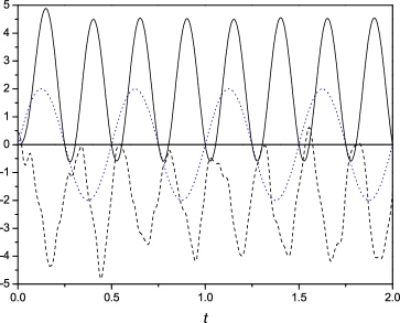
Figure 1: The response of the system to the oscillatory shear, in the linear response regime, which began at time $t=0$ following Eq. 8. The solid line is the entropy production, $\left\langle\Omega(t)\right\rangle=-\dot{\gamma}P_{xy}(t)V/\epsilon$. The dashed line is the instantaneous rate of heat absorbed by the thermostat $\left\langle dQ/dt\right\rangle/\epsilon$. The dotted line gives the strain rate $\dot{\gamma}(t)$ multiplied by a factor of 10. The data for the heat exchange is considerably more noisy than the other data. Clearly $\left\langle\Omega(t)\right\rangle$ is at times negative.

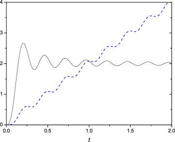
Figure 2: The dashed line is the integral, $\left\langle\bar{\Omega}_{t}\right\rangle t$, which is nonmonotonically increasing but always nonnegative. The solid line (black) is the time average $\left\langle\bar{\Omega}_{t}\right\rangle$ which is also always nonnegative.

In Fig. 1 the dissipation function, $\left\langle\Omega(t)\right\rangle$ in units of $k_{B}$ (which was calculated by ensemble averaging all of the nonequilibrium trajectories) is plotted as a function of time along with the ensemble averaged rate of heat absorbed by the thermostat, $\dot{Q}(t)=-3Nk_{B}T\left\langle\alpha(t)\right\rangle=k_{B}T\left\langle\Lambda\right\rangle$ in units of $\epsilon$. Also shown is the strain rate, $10\times\dot{\gamma}(t)$. The initial transients in the response decay very rapidly. It is clear that the response of the fluid is viscoelastic: there is a phase lag between $P_{xy}(t)$ and $\dot{\gamma}(t)$ due to the relatively high frequency $\omega$. This shows that the dissipation function (or at weak fields, equivalently, the entropy production Eq. 3) is negative within certain intervals of time even though the system’s response is linear. This effect is not due to the amplitude of the shear rate $\dot{\gamma}_{0}$ being large. This is clearly at odds with the traditional view from irreversible thermodynamics. In contrast Eq. 7 is satisfied at all times as may be seen in Fig. 2 where the integral $\left\langle\bar{\Omega}_{t}\right\rangle t$ and the time average $\left\langle\bar{\Omega}_{t}\right\rangle$ are plotted as a function of time $t$.

In summary we have shown the assertion of linear irreversible thermodynamics that the instantaneous entropy production is always nonnegative is incorrect for the case of time dependent viscoelastic fluids even if they are in the linear response regime close to equilibrium. The Second Law Inequality Eq. 7 derived from the Jarzynski Equality states that the time integral (starting from $t=0$) of the ensemble averaged dissipation function cannot be negative for arbitrary integration times and arbitrary field strengths (of course in the weak field limit the dissipation function is equal to the entropy production Eq. 3). This inequality requires that the Helmholtz free energy of the corresponding equilibrium system does not change. For planar shear this is a necessary condition for the fluid state, which by definition cannot support a constant stress. For a solid, undergoing oscillatory nonplastic deformation, the equilibrium free energy would depend on the deformation and the Clausius Inequality Eq. 6 will need to be used rather than the Second Law Inequality Eq. 7.

Lastly we note that the Second Law Inequality is a macroscopic consequence of the Jarzynski Equality and of the Evans Searles Fluctuation Theorem key-5 . All previously derived consequences of the JE and the Fluctuation Theorem were microscopic in nature. The Second Law Inequality in the form Eq. 7, has important consequences in applications such as atmospheric physics where the principle of maximum entropy in nonequilibrium states has been employed key-15 .

We thank the Australian Research Council for financial support, the Australian Partnership for Advanced Computing, and Debra J. Searles, Edie Sevick and Chris Jarzynski for helpful discussions. DJE thanks Siegfried Hess for reminding him of this problem.

References

-
(1)
Local equilibrium requires that the local thermodynamic
potentials are the same function of thermodynamic state variables
that they are in total equilibrium key-3 : in the case presented
here the same function of the thermostat temperature and the number
density. For an isotropic fluid variables such as the pressure, the
internal energy and the entropy do not change to linear order in the
amplitude of the external field regardless of the time dependence.
Thus the local equilibrium requirement and the linear response regime
are formely equivalent. This can be shown from response theory evans-morriss .
To linear order the average of the element of the pressure tensor
, for a process which begins at , is given by the Green
Kubo relation
where the notation denotes that the correlation function is determined for a system in equilibrium. Thermodynamic potentials are scalar variables which, in an isotropic fluid, do not change to linear order. If we denote a scalar variable as then, in an isotropic fluid, its cross correlation function with a tensor element has the the property, , due to symmetry. Thus to linear order in the external field scalar variables do not change,
Equivalently one may expand the distribution function as a Taylor series in the external field,
where is the equilibrium distribution function, and arrive at the same conclusion. This is shown in detail using Enskog theory in Ch IX, §6 of ref. key-3 . - (2) D. Kondepudi and I. Prigogine, Modern Thermodynamics (Wiley, New York, 1998); See especially Eq. (15.2.3).
- (3) S. R. De Groot and P. Mazur, Non-equilibrium Thermodynamics (Dover, New York, 1984).
- (4) P. J. Daivis and M. L. Matin, J. Chem. Phys. 118 (2003) 11111.
- (5) J. R. Dorfman, An Introduction to Chaos in Nonequilibrium Statistical Mechanics (Cambridge University Press, Cambridge, 1999).
- (6) C. Bustamante, J. Liphardt and F. Ritort, Phys. Today 58(7), 43 (2005).
- (7) D. Ruelle, Phys. Today 57(5) (2004) 48.
- (8) C. Jarzynski, Phys. Rev. Lett. 78 (1997) 2690.
- (9) C. Jarzynski, Phys. Rev. E 56 (1997) 5018.
- (10) D. J. Evans and G. P. Morriss, Statistical Mechanics of Nonequilibrium Liquids (Academic, London, 1990).
- (11) S. R. Williams, D. J. Searles and D. J. Evans, Phys. Rev. E 70 (2004) 066113.
- (12) D. J. Evans and D. J. Searles, Adv. Phys. 51 (2002) 1529.
- (13) D. J. Evans, Mol. Phys. 101 (2003) 1551.
- (14) J. Liphardt et. al., Science, 296 (2002) 1832.
- (15) D. Collin et. al., Nature, 437 (2005) 231.
- (16) D. J. Searles and D. J. Evans, Aust. J. Chem. 57 (2004) 1119.
- (17) R. Lorenz, Science, 299 (2003) 837.