Gilbert damping and spin Coulomb drag in a magnetized electron liquid with spin-orbit interaction

Abstract

We present a microscopic calculation of the Gilbert damping constant for the magnetization of a two-dimensional spin-polarized electron liquid in the presence of intrinsic spin-orbit interaction. First we show that the Gilbert constant can be expressed in terms of the auto-correlation function of the spin-orbit induced torque. Then we specialize to the case of the Rashba spin-orbit interaction and we show that the Gilbert constant in this model is related to the spin-channel conductivity. This allows us to study the Gilbert damping constant in different physical regimes, characterized by different orderings of the relevant energy scales – spin-orbit coupling, Zeeman coupling, momentum relaxation rate, spin-momentum relaxation rate, spin precession frequency – and to discuss its behavior in various limits. Particular attention is paid to electron-electron interaction effects, which enter the spin conductivity and hence the Gilbert damping constant via the spin Coulomb drag coefficient.

I Introduction

The Gilbert constant characterizing the damping of magnetization precession is one of the important phenomenological parameters that describe the collective magnetization dynamics of ferromagnets.Gilbert (1955, 2004); Lifshitz and Pitaevskii (1980). It is an essential input of the Landau-Lifshitz-Gilbert equation (LLG) for magnetization dynamicsLifshitz and Pitaevskii (1980) and as such is widely used in the analysis of magnetization reversal processes, which are crucial to magnetic recording technologies Tserkovnyak et al. (2005). Recently, hybrid systems of ferromagnets and normal metals have also attracted considerable attention, in the context of the enhancement of Gilbert damping at the ferromagnet-normal metal interfaces.Tserkovnyak et al. (2002a, b); Tserkovnyak et al. (2005) Despite tremendous efforts to elucidate the nature of Gilbert damping in bulk ferromagnets, however, the microscopic processes responsible for the observed ferromagnetic relaxation in real materials are still not fully understood. The matter is complicated by the potential relevance of a number of different mechanisms involving eddy currents, magnetoelastic coupling, two-magnon and nonlinear multimagnon processes, extrinsic and intrinsic spin-orbit (SO) coupling of itinerant electrons.Heinrich et al. (1967); Korenman and Prange (1972); Lutovinov and Reizer (1979); Solontsov and Vasil’ev (1993); Suhl (1998); Heinrich et al. (2002); Kuneš and Kamberský (2002); Dobin and Victora (2003); Sinova et al. (2004a); Tserkovnyak et al. (2004); Koopmans et al. (2005); Steiauf and Fähnle (2005); Tserkovnyak et al. ; Kohno et al. Without delving into a detailed discussion of various points of view, we note that a certain level of consensus has been reached in the recent theoretical literature about the central importance of SO interaction of some form in conducting ferromagnets, although with a limited and rather indirect experimental support at present.Mizukami et al. (2002); Ingvarsson et al. (2002)

Even restricting the attention to the SO-based mechanisms of Gilbert damping, however, the myriad of relevant energy scales (namely, ferromagnetic resonance frequency, ferromagnetic exchange energy, intrinsic SO splitting, impurity scattering rate, and spin dephasing due to magnetic or SO disorder) has led different authors to make qualitatively different predictions for the Gilbert damping, for example, with regard to its dependence on the disorder strength.Heinrich et al. (1967); Kuneš and Kamberský (2002); Sinova et al. (2004a); Burkov and Balents (2004); Tserkovnyak et al. (2004); Kohno et al. . Furthermore, electron-electron ($e-e$) interactions have mainly been discussed in the mean-field spirit, as the source of the exchange field in itinerant-electron ferromagnets.

In this paper, we set off to formulate a microscopic theory of the Gilbert damping constant, which we then apply to a simple model, where the competition of different energy scales can be studied, comparing various points of view and also generalizing and extending the results existing in the literature. We wish to consider the interplay of magnetic spin splitting, intrinsic SO strength, disorder scattering, as well as the strength of $e-e$ interactions in a single self-contained model without introducing any phenomenological dephasing or relaxation parameters. In particular, we find an intricate relation between the spin-drag correlations induced by $e-e$ interactions and the Gilbert damping in two-dimensional electron liquids. We hope our discussion will bring the community a step closer to understanding the relevant microscopic mechanisms responsible for the Gilbert damping observed in conducting ferromagnets and spin-polarized systems.

SO interactions, especially in narrow-band semiconductors, have recently received a great deal of attention in the context of spin-based electronics (i.e., spintronics). In particular, theoretical proposals to manipulate spins by means of intrinsic SO interactions, without the use of magnetic fields or magnetic materials, especially in the so-called spin Hall configuration,Murakami et al. (2003); Sinova et al. (2004b) have unleashed a wave of theoretical research as well as experimental efforts to measure the effect.Kato et al. (2004); Wunderlich et al. (2005); Sih et al. (2006) It is worthwhile noting that these activities have shown the need to better understand the fundamental aspects of intrinsic SO coupling and its experimental manifestations. The role of $e-e$ interactions, furthermore, remains a relatively unexplored territory with regard to its interplay with interesting topological properties brought about by the SO coupling, which lie beyond the conventional theories of electron liquids. In addition, the recent discovery of the Aharonov-Casher phaseKonig et al. (2006) in narrow-band semiconductors shows that a study of the combined response to magnetic and SO fields in a regime of weak and strong SO interactions is of urgent importance. It is closely related to the topic considered here, i.e., the spin response and relaxation in magnetized system with SO interactions.

In this paper, we study an interacting electron liquid magnetized by an external magnetic field in the presence of SO interactions. First, by comparing the macroscopic Landau-Lifshitz-Gilbert (LLG) theory with a microscopically derived expression for the transverse spin susceptibility, we find the following relationship between the Gilbert damping constant and the torque-torque correlator (see Eq. 32 below):

$$\lambda=-\frac{g}{M_{0}V}\lim_{\omega\to 0}\Im m\frac{\langle\langle\hat{\tau};\hat{\tau}\rangle\rangle_{\omega}}{\omega}$$ (1)

where $g$ is the gyromagnetic ratio, $\lambda$ is the dimensionless Gilbert coefficient, $M_{0}$ is the equilibrium magnetization, $V$ the volume of the system, and $\hat{\tau}$ the torque induced by SO interactions. To derive Eq. (1) we must neglect certain contributions of order higher than the fourth in the strength of the spin-orbit coupling: we will argue that this procedure is justified, not only at zero frequency but also at frequencies close to the ferromagnetic resonance.

Next we focus on the specific case of a two-dimensional electron gas (2DEG) with Rashba SO interactions induced by a uniform electric field perpendicular to the plane of the electron gas. In this case, we show that the Gilbert damping constant can be expressed in terms of the spin-channel conductivity: the same result holds in a three-dimensional electron gas, provided the electric field responsible for the spin-orbit interaction is uniform in space. For the isotropic case, i.e., when the magnetic field, the magnetization, and the SO-inducing electric field are all perpendicular to the direction of the 2DEG, the result is

$$\lambda=\frac{\bar{\alpha}^{2}E_{F}\tau}{\hbar p}\frac{\Re e\sigma_{s\parallel}(0)}{\sigma_{D}}\,,$$ (2)

where $E_{F}$ is the Fermi energy, $\tau$ is the momentum relaxation time due to electron-impurity scattering, $\bar{\alpha}$ is the Rashba SO-coupling strength normalized by the Fermi velocity $v_{F}$, $p$ is the degree of spin polarization, $\sigma_{D}$ is the Drude conductivity, and $\sigma_{s\parallel}(0)$ is the longitudinal spin-channel conductivity.

The problem now shifts to the calculation of the spin-channel conductivity. We show that this can be done exactly (subject to the usual weak-disorder assumption $E_{F}\tau\gg 1$) in the isotropic non-interacting case, with ladder vertex corrections playing an essential role in ensuring the correct behavior in the limit of strong SO coupling. $e-e$ interactions can then be introduced using the formalism described in Refs. D’Amico and Vignale, 2000, 2002. The final result for the isotropic case at zero frequency has the form:

$$\lambda=\frac{p\bar{\alpha}^{2}E_{F}\tau}{\hbar(p^{2}+\bar{\alpha}^{2})}\frac{1+\frac{1}{2}(\Omega\tau)^{2}(1+\cos^{2}\delta)}{\cos^{2}\delta+\frac{1}{4}(\Omega\tau)^{2}(1+\cos^{2}\delta)^{2}}\frac{1+p^{2}\gamma\tau}{1+\gamma\tau}\,,$$ (3)

where $\Omega$ is the spin splitting of electronic states due to the combined action of the external magnetic field and the SO effective magnetic field, $\cos\delta$ is the ratio of the external magnetic field to the total effective field $\Omega$, and $\gamma$ is the spin-drag coefficient. This expresses the Gilbert damping as a function of disorder strength, magnetic field, SO and $e-e$ interactions.

One of the gross features of Eq. (3) is a rough scaling of $\lambda$ with $\tau$, which is particularly evident in the clean limit $\tau\to\infty$. We will see, however, that Eq. (3) describes in general a nonmonotonic dependence of $\lambda$ on the scattering rate, due to the interplay between $1/\tau$ and other energy scales. For example, in the regime of strong $e-e$ interactions and weak polarizations, $1<\gamma\tau<1/p^{2}$, the Gilbert damping $\lambda$ becomes independent of $\tau$ and scales as $1/\gamma$.

It is important to note that Eq. (3) holds in the low-frequency limit, $\omega\to 0$, which means in practice $\omega$ much smaller than all the other energy scales. For this reason the divergence of $\lambda$ as $1/\tau\to 0$ in Eq. (3), which was obtained after first taking the $\omega\to 0$ limit, is not physically consequential: taking the $1/\tau\to 0$ limit with a fixed $\omega$ results in a vanishing damping as it should.Tserkovnyak et al. (2004). This is clearly seen by extending the calculation of $\lambda$ to finite frequency, which can be done with little extra effort in the $\omega\ll E_{F}$ regime. This important extension of Eq. (3) is presented in full in Eq. 59 below. Among other modifications we get a factor $\frac{1}{1+(\omega\tau)^{2}}$ to multiply Eq. (3), ensuring the correct behavior of $\lambda$ for $\tau\to\infty$ at finite $\omega$.

The rest of the paper is organized as follows. In Sec. II, we discuss the LLG phenomenology, which is compared to the microscopic calculation in Sec. III, allowing us to express the Gilbert damping constant in terms of the torque-torque correlator. In Sec. IV.1, we present the calculation of the Gilbert damping constant in the presence of the Rashba SO and $e-e$ interactions for an isotropic case, i.e., when the magnetic field is perpendicular to the 2DEG plane. In Sec. IV.2, the same model is treated for the anisotropic case, where the induced magnetization is tilted away from the direction perpendicular to the 2DEG. Our summary, conclusions and speculations are presented in Sec. V. Technical details of the calculations are supplied in the Appendixes.

II LLG equation

Studies of the magnetization dynamics in ferromagnetic materials often start from a phenomenological equation of motion for the magnetization

$${\bf M}({\bf r},t)=-g\langle\mathbf{\hat{s}}({\bf r},t)\rangle\,,$$ (4)

where $\langle\mathbf{\hat{s}}({\bf r},t)\rangle$ is the expectation value of the spin-density operator at position ${\bf r}$ and $g$ is the gyromagnetic ratio: for free electrons in vacuum, $g=e/mc$ where $e$ is the absolute value of the electron charge. An important assumption in the LLG phenomenology is that the magnitude of the magnetization is fixed at a constant value $M_{0}$ (determined by the minimization of the free energy), i.e., we have

$${\bf M}=M_{0}{\bf\hat{e}_{M}}\,,$$ (5)

where ${\bf\hat{e}_{M}}$ is the unit vector specifying the direction of the magnetization. The physical reasoningLifshitz and Pitaevskii (1980) underlying this picture assumes a very large (essentially infinite) longitudinal spin stiffness which prevents changes in the magnitude of ${\bf M}$, while one focuses on the softer transverse modes – essentially ferromagnetic Goldstone modes with a finite gap in the presence of intrinsic or extrinsic anisotropies. The direction of the magnetization ${\bf\hat{e}_{M}}$ thus provides the relevant degrees of freedom, whose time evolution is determined by the LLG equation

$$\frac{\partial{\bf\hat{e}_{M}}}{\partial t}=g{\bf H}_{\rm eff}\times{\bf\hat{e}_{M}}+\stackrel{{\scriptstyle\leftrightarrow}}{{\lambda}}\cdot\,{\bf\hat{e}_{M}}\times\frac{\partial{\bf\hat{e}_{M}}}{\partial t}\,,$$ (6)

where ${\bf H}_{\rm eff}$ is the effective magnetic field defined as the functional derivative of the equilibrium free-energy density $f({\bf M})$, regarded as a functional of the magnetization ${\bf M}$, with respect to its argument:

$${\bf H}_{\rm eff}({\bf r},t)=-\frac{\delta f({\bf M})}{\delta{\bf M}({\bf r},t)}\,.$$ (7)

$\stackrel{{\scriptstyle\leftrightarrow}}{{\lambda}}$ is a symmetric $2\times 2$ matrix acting in the two-dimensional space perpendicular to the magnetization, and the dot denotes the usual matrix product [note that the possible antisymmetric component of $\stackrel{{\scriptstyle\leftrightarrow}}{{\lambda}}$ would only lead to a renormalization of the gyromagnetic ratio in Eq. (7).] The first term on the right-hand side (r.h.s.) of this equation produces a coherent precessional motion of the magnetization, conserving the total free energy, while the second term, known as the Gilbert damping, is responsible for the relaxation toward equilibrium, i.e., the lowest free-energy state. Both terms vanish at equilibrium. Notice that the LLG equation is not restricted to the linear-response regime, as ${\bf\hat{e}_{M}}$ is allowed to wander away arbitrarily from the equilibrium orientation.

The primary focus of this paper is on the microscopic calculation of the Gilbert damping matrix $\stackrel{{\scriptstyle\leftrightarrow}}{{\lambda}}$. We concentrate exclusively on homogeneous systems, that is the situation in which ${\bf M}$ is independent of position and depends only on time. In such a case, it is immediately obvious that any damping must arise from the coupling between the spin and the orbital degrees of freedom. This is so since the nonrelativistic $e-e$ interaction is invariant under a uniform rotation of all the spins, and thus cannot be involved in the damping of such a rotation. It will therefore be essential to include the SO coupling in our microscopic calculation, and we will do this starting from the simplest model, and then try to generalize our conclusions to more realistic situations. Note that although in our model we consider SO coupling stemming from the relativistic corrections to the Schrödinger equation, a kind of SO coupling would also be possible in the presence of an inhomogeneous crystal magnetic field.

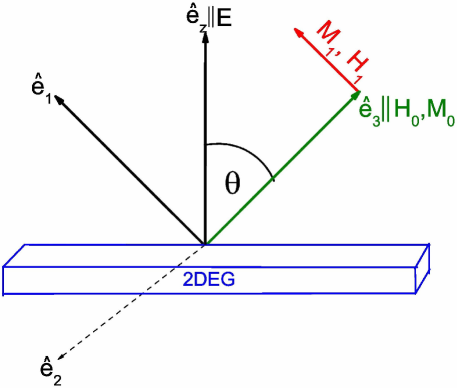
Figure 1: The directions of the magnetic and Rashba fields in relation to the 2DEG plane, the model which we discuss in Section IV. Also, visualization of directions of equilibrium and induced magnetization presented in Eqs. 8-14.

We can calculate $\stackrel{{\scriptstyle\leftrightarrow}}{{\lambda}}$ by applying Eq. (6) to a linear-response problem and comparing the resulting susceptibility with the susceptibility obtained from the Kubo formula. Our linear-response problem is depicted in Fig. 1. We perturb the system with a small magnetic field ${\bf H}_{1}$ perpendicular to the direction of the equilibrium magnetization, which we denote by ${\bf\hat{e}_{3}}$ to distinguish it from the actual direction of the magnetization ${\bf\hat{e}_{M}}$. ${\bf H}_{1}$ is uniform in space and periodic in time, with an angular frequency $\omega$ (this field must not be confused with the static field ${\bf H}_{0}$ which may be present at equilibrium). In response to ${\bf H}_{1}$, the direction of the magnetization becomes time dependent and will be written as

$${\bf\hat{e}_{M}}(t)={\bf\hat{e}_{3}}+{\bf\delta\hat{e}_{M}}(t)\,,$$ (8)

where ${\bf\delta\hat{e}_{M}}$ is a small vector perpendicular to ${\bf\hat{e}_{3}}$, which therefore does not change the normalization of ${\bf\hat{e}_{M}}$ to first order. Adding the external field ${\bf H}_{1}$ to ${\bf H}_{\rm eff}$ and substituting Eq. (8) into Eq. (6), we obtain the equation of motion for ${\bf\delta\hat{e}_{M}}$ to first order in ${\bf H}_{1}$:

$$\frac{\partial{\bf\delta\hat{e}_{M}}}{\partial t}=g({\bf H}_{1}+{\bf H}_{\rm eff,1})\times{\bf\hat{e}_{3}}+\stackrel{{\scriptstyle\leftrightarrow}}{{\lambda}}\cdot\,{\bf\hat{e}_{3}}\times\frac{\partial{\bf\delta\hat{e}_{M}}}{\partial t}\,.$$ (9)

To the same order, the effective field is

$${\bf H}_{\rm eff,1} = -\frac{1}{M_{0}^{2}}\left.\frac{\partial^{2}f({\bf M})}{\partial{\bf\hat{e}_{M}}\partial{\bf\hat{e}_{M}}}\right|_{{\bf\hat{e}_{3}}}\cdot M_{0}{\bf\delta\hat{e}_{M}}$$ (10)

$$= -\stackrel{{\scriptstyle\leftrightarrow}}{{S}}\cdot M_{0}{\bf\delta\hat{e}_{M}}\,,$$

where we have defined the transverse spin stiffness matrix

$$\stackrel{{\scriptstyle\leftrightarrow}}{{S}}\equiv\frac{1}{M_{0}^{2}}\left.\frac{\partial^{2}f({\bf M})}{\partial{\bf\hat{e}_{M}}\partial{\bf\hat{e}_{M}}}\right|_{{\bf\hat{e}_{3}}}\,,$$ (11)

a $2\times 2$ matrix in the plane perpendicular to ${\bf\hat{e}_{3}}$.

Upon taking a Fourier transform with respect to time, the linearized LLG equation can be rewritten as follows:

$$\left[-i\omega(\stackrel{{\scriptstyle\leftrightarrow}}{{1}}+\stackrel{{\scriptstyle\leftrightarrow}}{{\epsilon}}\cdot\stackrel{{\scriptstyle\leftrightarrow}}{{\lambda}})+gM_{0}\stackrel{{\scriptstyle\leftrightarrow}}{{\epsilon}}\cdot\stackrel{{\scriptstyle\leftrightarrow}}{{S}}\right]\cdot{\bf\delta\hat{e}_{M}}=g\stackrel{{\scriptstyle\leftrightarrow}}{{\epsilon}}\cdot\,{\bf H}_{1}\,,$$ (12)

where $\stackrel{{\scriptstyle\leftrightarrow}}{{1}}$ is the $2\times 2$ identity matrix and

$$\stackrel{{\scriptstyle\leftrightarrow}}{{\epsilon}}\equiv\left(\begin{array}[]{cc}0&1\\ -1&0\end{array}\right)\,,$$ (13)

$\stackrel{{\scriptstyle\leftrightarrow}}{{\epsilon}}^{-1}=-\stackrel{{\scriptstyle\leftrightarrow}}{{\epsilon}}$. The transverse spin susceptibility $\stackrel{{\scriptstyle\leftrightarrow}}{{\chi}}$ connects the transverse magnetization ${\bf M}_{1}=M_{0}{\bf\delta\hat{e}_{M}}$ to the external field ${\bf H}_{1}$:

$${\bf M}_{1}(\omega)=\stackrel{{\scriptstyle\leftrightarrow}}{{\chi}}(\omega)\cdot{\bf H}_{1}(\omega)\,.$$ (14)

Comparing this with Eq. (12), we easily obtain

$$\stackrel{{\scriptstyle\leftrightarrow}}{{\chi}}^{-1}(\omega)=\frac{i\omega(\stackrel{{\scriptstyle\leftrightarrow}}{{\epsilon}}-\stackrel{{\scriptstyle\leftrightarrow}}{{\lambda}})}{gM_{0}}+\stackrel{{\scriptstyle\leftrightarrow}}{{S}}\,,$$ (15)

which is the most general form of the anisotropic transverse response, to the first order in frequency. Notice that $\stackrel{{\scriptstyle\leftrightarrow}}{{\chi}}^{-1}(0)=\stackrel{{\scriptstyle\leftrightarrow}}{{S}}$, showing that the transverse stiffness is indeed the inverse of the static spin susceptibility. In an isotropic system, $\stackrel{{\scriptstyle\leftrightarrow}}{{S}}$ vanishes (the free energy does not depend on the direction of the magnetization). If a static external field ${\bf H}_{0}=H_{0}{\bf\hat{e}_{3}}$ is applied to such a system, then the stiffness matrix becomes $\stackrel{{\scriptstyle\leftrightarrow}}{{S}}=(H_{0}/M_{0})\stackrel{{\scriptstyle\leftrightarrow}}{{1}}$. Anisotropies due to SO interactions will show up as additional contributions to $\stackrel{{\scriptstyle\leftrightarrow}}{{S}}$.

Needless to say, the theory described in this section is valid only at low frequencies (in comparison to relevant microscopic energy scales), when the frequency expansion of the inverse susceptibility, such as Eq. (15), can be truncated at the linear term.

III Microscopic theory

A microscopic expression for the homogeneous transverse spin susceptibility is given by the Kubo formula

$$\chi_{ij}(\omega)=\frac{g^{2}}{V}\left[\frac{i}{\hbar}\int_{0}^{\infty}dt\langle[\hat{S}_{i}(t),\hat{S}_{j}(0)]\rangle e^{i(\omega+i0^{+})t}\right]\,,$$ (16)

where $\hat{S}_{i}(t)$ is the Heisenberg operator of the total spin of the system, the angular bracket denotes the equilibrium average, $V$ is the volume of the system, and $i$, $j$ are Cartesian indices in the plane perpendicular to the magnetization (they can take up the values $1$ or $2$). The lengthy expression inside the square brackets in the above equation (i.e., the retarded spin response function) will be abbreviated from now on as $-\langle\langle\hat{S}_{i};\hat{S}_{j}\rangle\rangle_{\omega}$, so we have

$$\chi_{ij}(\omega)=-\frac{g^{2}}{V}\langle\langle\hat{S}_{i};\hat{S}_{j}\rangle\rangle_{\omega}\,.$$ (17)

(The magnetization is related to the average spin by ${\bf M}=-g\langle{\bf\hat{S}}\rangle/V$.) Notice that this expression is dimensionless in three dimensions and has the units of length in two spatial dimensions (in the cgs units).

In view of the fact that Gilbert damping arises ultimately from torques on the individual spins, it is convenient to rewrite Eq. (17) in terms of the time derivatives of ${\bf\hat{S}}$. The time derivative of the spin is conveniently written as the sum of two parts: a free precession term at frequency $\omega_{0}$ about the magnetization axis ${\bf\hat{e}_{3}}$ and a residual torque $\hat{\tau}$ due to the SO interactions:

$${\bf\dot{\hat{S}}}=\omega_{0}{\bf\hat{e}_{3}}\times{\bf\hat{S}}+\mbox{{\boldmath$\hat{\tau}$}}\,.$$ (18)

Here, $\omega_{0}=gH_{0}^{\prime}$, where $H_{0}^{\prime}$ is the projection of the static magnetic field along ${\bf\hat{e}_{3}}$, while $\hat{\tau}$ is a model-dependent torque, which is proportional to the spin-orbit coupling constant.

It is very convenient at this point to rewrite Eq. (17) in terms of the $\langle\langle\mbox{{\boldmath$\hat{\tau}$}};\mbox{{\boldmath$\hat{\tau}$}}\rangle\rangle$ correlation function. The fact that $\hat{\tau}$ explicitly contains the spin-orbit coupling constant $\alpha$ will allow us to calculate the correlator, to order $\alpha^{2}$, without including the spin-orbit interaction in the hamiltonian: this will be a major simplification. Furthermore, this transformation will enable us to connect the Gilbert constant to the spin conductivity, which is particularly helpful for the inclusion of $e-e$ interactions.

To express the spin susceptibility in terms of the $\langle\langle\mbox{{\boldmath$\hat{\tau}$}};\mbox{{\boldmath$\hat{\tau}$}}\rangle\rangle$ correlator we make use of the identity

$$\langle\langle\hat{A};\hat{B}\rangle\rangle_{\omega} = -\frac{\langle\langle\dot{\hat{A}};\hat{B}\rangle\rangle_{\omega}}{i\omega}+\frac{\langle[\hat{A},\hat{B}]\rangle}{\hbar\omega}$$ (19)

$$= +\frac{\langle\langle{\hat{A}};\dot{\hat{B}}\rangle\rangle_{\omega}}{i\omega}+\frac{\langle[\hat{A},\hat{B}]\rangle}{\hbar\omega}\,,$$

where

$$\dot{\hat{A}}=\frac{1}{i\hbar}[\hat{A},\hat{H}]$$ (20)

is the time derivative of $\hat{A}$ and $\hat{H}$ is the unperturbed Hamiltonian.

Combining Eqs. (19) and (18), we easily obtain

$$-i\omega\langle\langle\hat{S}_{i};\hat{S}_{j}\rangle\rangle_{\omega}=\langle\langle\dot{\hat{S}}_{i};\hat{S}_{j}\rangle\rangle_{\omega}-\frac{i}{\hbar}\langle[\hat{S}_{i},\hat{S}_{j}]\rangle$$ (21)

$$= \epsilon_{ij}\langle\hat{S}_{3}\rangle-\omega_{0}\epsilon_{ik}\langle\langle\hat{S}_{k};\hat{S}_{j}\rangle\rangle_{\omega}+\langle\langle\hat{\tau}_{i};\hat{S}_{j}\rangle\rangle_{\omega}\,,$$

where a sum over the repeated index ($k$ in this case) is understood. Solving for $\langle\langle\hat{S}_{i};\hat{S}_{j}\rangle\rangle_{\omega}$, we get

$$\langle\langle\hat{S}_{i};\hat{S}_{j}\rangle\rangle_{\omega}=-\frac{i\omega\delta_{ik}+\omega_{0}\epsilon_{ik}}{\omega^{2}_{0}-\omega^{2}}\left[\epsilon_{kj}\langle\hat{S}_{3}\rangle+\langle\langle\hat{\tau}_{k};\hat{S}_{j}\rangle\rangle_{\omega}\right]\,.$$ (22)

In the absence of the SO coupling, the torque $\hat{\tau}$ vanishes and the second term on the r.h.s. of Eq. (22) is absent. Then the susceptibility is easily found to have the form

$$\chi^{(0)}_{ij}(\omega)=gM_{0}\frac{-i\omega\epsilon_{ij}+\omega_{0}\delta_{ij}}{\omega_{0}^{2}-\omega^{2}}~{}.$$ (23)

Notice that its inverse

$$[\stackrel{{\scriptstyle\leftrightarrow}}{{\chi}}^{(0)}]^{-1}(\omega)=\frac{i\omega\stackrel{{\scriptstyle\leftrightarrow}}{{\epsilon}}+\omega_{0}\stackrel{{\scriptstyle\leftrightarrow}}{{1}}}{gM_{0}}$$ (24)

is in a perfect agreement with Eq. (15), if in the latter we set $\stackrel{{\scriptstyle\leftrightarrow}}{{\lambda}}=0$ and $\stackrel{{\scriptstyle\leftrightarrow}}{{S}}=(\omega_{0}/gM_{0})\stackrel{{\scriptstyle\leftrightarrow}}{{1}}$.

Upon applying again Eq. (19) to $\langle\langle\hat{\tau}_{k};\hat{S}_{j}\rangle\rangle_{\omega}$, we get

$$\langle\langle\hat{\tau}_{k};\hat{S}_{j}\rangle\rangle_{\omega}=\left[\frac{i}{\hbar}\langle[\hat{\tau}_{k},\hat{S}_{l}]\rangle+\langle\langle\hat{\tau}_{k};\hat{\tau}_{l}\rangle\rangle_{\omega}\right]\frac{i\omega\delta_{lj}+\omega_{0}\epsilon_{lj}}{\omega^{2}_{0}-\omega^{2}}\,,$$ (25)

Putting this in Eq. (22) and making use of Eqs. (17) and (23), we arrive after some algebraic manipulations at the following compact formula for the spin susceptibility matrix:

$$\stackrel{{\scriptstyle\leftrightarrow}}{{\chi}}(\omega)=\stackrel{{\scriptstyle\leftrightarrow}}{{\chi}}^{(0)}(\omega)+\stackrel{{\scriptstyle\leftrightarrow}}{{\chi}}^{(0)}(\omega)\cdot\frac{\stackrel{{\scriptstyle\leftrightarrow}}{{\epsilon}}\cdot\stackrel{{\scriptstyle\leftrightarrow}}{{\Gamma}}(\omega)\cdot\stackrel{{\scriptstyle\leftrightarrow}}{{\epsilon}}}{M_{0}^{2}V}\cdot\stackrel{{\scriptstyle\leftrightarrow}}{{\chi}}^{(0)}(\omega)\,,$$ (26)

where the matrix $\stackrel{{\scriptstyle\leftrightarrow}}{{\Gamma}}(\omega)$ is defined as follows:

$$\Gamma_{ij}(\omega)=\langle\langle\hat{\tau}_{i};\hat{\tau}_{j}\rangle\rangle_{\omega}+\frac{i}{\hbar}\langle[\hat{\tau}_{i},\hat{S}_{j}]\rangle\,.$$ (27)

The main dynamical quantity on the r.h.s. here is the torque-torque response function $\langle\langle\hat{\tau}_{i};\hat{\tau}_{j}\rangle\rangle_{\omega}$. The rest is ground-state averages that we will not be interested in.

We can now express the Gilbert damping and stiffness matrices, $\stackrel{{\scriptstyle\leftrightarrow}}{{\lambda}}$ and $\stackrel{{\scriptstyle\leftrightarrow}}{{S}}$, which appear in the phenomenological equation (15), in terms of microscopic response functions. First of all, consider the formal limit of weak SO interactions. In this limit, $\stackrel{{\scriptstyle\leftrightarrow}}{{\Gamma}}$, which is proportional to the square of the SO coupling constant, is assumed to give a small correction to the susceptibility (we will comment below on the conditions of applicability of this regime). Upon inverting Eq. (26) to first order in $\stackrel{{\scriptstyle\leftrightarrow}}{{\Gamma}}$, we obtain

$$\stackrel{{\scriptstyle\leftrightarrow}}{{\chi}}^{-1}(\omega)\simeq[\stackrel{{\scriptstyle\leftrightarrow}}{{\chi}}^{(0)}]^{-1}(\omega)-\frac{\stackrel{{\scriptstyle\leftrightarrow}}{{\epsilon}}\cdot\stackrel{{\scriptstyle\leftrightarrow}}{{\Gamma}}(\omega)\cdot\stackrel{{\scriptstyle\leftrightarrow}}{{\epsilon}}}{M_{0}^{2}V}\,.$$ (28)

Comparing this with Eq. (15), and taking into account Eq. (24), we get

$$\stackrel{{\scriptstyle\leftrightarrow}}{{S}}_{so}=-\frac{\stackrel{{\scriptstyle\leftrightarrow}}{{\epsilon}}\cdot\stackrel{{\scriptstyle\leftrightarrow}}{{\Gamma}}(0)\cdot\stackrel{{\scriptstyle\leftrightarrow}}{{\epsilon}}}{M_{0}^{2}V}$$ (29)

and

$$\stackrel{{\scriptstyle\leftrightarrow}}{{\lambda}}=\frac{g}{M_{0}V}\lim_{\omega\to 0}\left.\Im m\frac{\stackrel{{\scriptstyle\leftrightarrow}}{{\epsilon}}\cdot\stackrel{{\scriptstyle\leftrightarrow}}{{\Gamma}}(\omega)\cdot\stackrel{{\scriptstyle\leftrightarrow}}{{\epsilon}}}{\omega}\right|_{sym}\,,$$ (30)

where the subscript $sym$ denotes the symmetric part of a matrix. In the first of these two equations, $\hat{S}_{so}$ is the SO contribution to the stiffness matrix, i.e., $\stackrel{{\scriptstyle\leftrightarrow}}{{S}}_{so}\equiv\stackrel{{\scriptstyle\leftrightarrow}}{{S}}-(H_{0}^{\prime}/M_{0})\stackrel{{\scriptstyle\leftrightarrow}}{{1}}$, which reflects SO induced magnetic anisotropy. The second equation is the main result at this point. It expresses the Gilbert damping matrix in terms of the zero-frequency slope of the spectrum of the torque-torque response function. Notice that this spectrum has no contribution from the second term on the r.h.s. of Eq. (27), which is purely real (the commutator of two hermitian operators is anti-hermitian). In general, the imaginary part of $\stackrel{{\scriptstyle\leftrightarrow}}{{\epsilon}}\cdot\stackrel{{\scriptstyle\leftrightarrow}}{{\Gamma}}(\omega)\cdot\stackrel{{\scriptstyle\leftrightarrow}}{{\epsilon}}$ will have both symmetric and antisymmetric components: the latter has been interpreted as a Berry curvature correctionQian and Vignale (2002) to the adiabatic spin dynamics [also, see the note below Eq. (7), where we point out that inclusion of the antisymmetric component would lead to a renormalization of the $g$-factor]. The symmetric component is purely diagonal in the limit of weak spin-orbit coupling because in this limit the system is isotropic under rotations about the $3$ axis. (In general, one can still diagonalize the symmetric component of the spectrum by a suitable choice of the axes in the $1-2$ plane – a transformation that does not affect the antisymmetric component. We will not consider this complication here). Thus we conclude that the Gilbert damping matrix is a diagonal matrix of the form

$$\stackrel{{\scriptstyle\leftrightarrow}}{{\lambda}}\equiv\left(\begin{array}[]{cc}\lambda_{1}&0\\ 0&\lambda_{2}\end{array}\right)\,,$$ (31)

where

$$\lambda_{1}=-\frac{g}{M_{0}V}\lim_{\omega\to 0}\Im m\frac{\langle\langle\hat{\tau}_{2};\hat{\tau}_{2}\rangle\rangle_{\omega}}{\omega}$$ (32)

and

$$\lambda_{2}=-\frac{g}{M_{0}V}\lim_{\omega\to 0}\Im m\frac{\langle\langle\hat{\tau}_{1};\hat{\tau}_{1}\rangle\rangle_{\omega}}{\omega}\,.$$ (33)

The above formulas have been derived from a first order expansion in $\stackrel{{\scriptstyle\leftrightarrow}}{{\Gamma}}$, which is justified for $\omega\ll\omega_{0}$ when the spin-orbit interaction is weak. At first sight, however, the approximation seems to break down completely when $\omega\sim\omega_{0}$ (the interesting region of the ferromagnetic resonance) because $\stackrel{{\scriptstyle\leftrightarrow}}{{\chi}}^{(0)}$ has a pole at $\omega=\omega_{0}$. But this conclusion is too hasty. To show this, we first notice that the exact inversion of $\stackrel{{\scriptstyle\leftrightarrow}}{{\chi}}$ from Eq. (26) gives

$$\stackrel{{\scriptstyle\leftrightarrow}}{{\chi}}^{-1}(\omega)=[\stackrel{{\scriptstyle\leftrightarrow}}{{\chi}}^{(0)}]^{-1}(\omega)-\stackrel{{\scriptstyle\leftrightarrow}}{{\Sigma}}(\omega)\,$$ (34)

where the “self-energy” $\stackrel{{\scriptstyle\leftrightarrow}}{{\Sigma}}(\omega)$ is given by

$$\stackrel{{\scriptstyle\leftrightarrow}}{{\Sigma}}(\omega)=\frac{\stackrel{{\scriptstyle\leftrightarrow}}{{\epsilon}}\cdot\stackrel{{\scriptstyle\leftrightarrow}}{{\Gamma}}(\omega)\cdot\stackrel{{\scriptstyle\leftrightarrow}}{{\epsilon}}}{M_{0}^{2}V}\left[\stackrel{{\scriptstyle\leftrightarrow}}{{1}}+\stackrel{{\scriptstyle\leftrightarrow}}{{\chi}}^{(0)}(\omega)\cdot\frac{\stackrel{{\scriptstyle\leftrightarrow}}{{\epsilon}}\cdot\stackrel{{\scriptstyle\leftrightarrow}}{{\Gamma}}(\omega)\cdot\stackrel{{\scriptstyle\leftrightarrow}}{{\epsilon}}}{M_{0}^{2}V}\right]^{-1}\,.\\$$ (35)

For $\omega\ll\omega_{0}$, $\stackrel{{\scriptstyle\leftrightarrow}}{{\chi}}^{(0)}(\omega)$ reduces to $S_{0}^{-1}=\frac{gM_{0}}{\omega_{0}}$, which is just the inverse of the stiffness to zero-th order in the spin-orbit interaction. Then, from the above formulas and making use of Eq. (29) we see that the zero-frequency Gilbert matrix (proportional to $\Im m\stackrel{{\scriptstyle\leftrightarrow}}{{\Sigma}}(\omega)/\omega$) is given by Eq. (30) times a renormalization factor

$$\left(\stackrel{{\scriptstyle\leftrightarrow}}{{1}}-\frac{\stackrel{{\scriptstyle\leftrightarrow}}{{S}}_{so}}{S_{0}}\right)^{-1}~{}.$$ (36)

We will estimate this renormalization below for a specific model, and find it to be very small.

An important observation is that, unlike the function $\stackrel{{\scriptstyle\leftrightarrow}}{{\chi}}^{(0)}(\omega)$, the self-energy is well-behaved at $\omega=\omega_{0}$. Indeed from Eq. (26) we see that $\stackrel{{\scriptstyle\leftrightarrow}}{{\Gamma}}(\omega)$ must vanish at $\omega_{0}$ in order to cancel the pole of $\stackrel{{\scriptstyle\leftrightarrow}}{{\chi}}^{(0)}$ and replace it with a roughly Lorentzian peak at the true ferromagnetic resonance. Furthermore, the rate at which $\stackrel{{\scriptstyle\leftrightarrow}}{{\Gamma}}(\omega)$ vanishes for $\omega$ tending to $\omega_{0}$ must be such that the denominator of Eq. (35), i.e., $\left[\stackrel{{\scriptstyle\leftrightarrow}}{{1}}+\stackrel{{\scriptstyle\leftrightarrow}}{{\chi}}^{(0)}(\omega)\cdot\frac{\stackrel{{\scriptstyle\leftrightarrow}}{{\epsilon}}\cdot\stackrel{{\scriptstyle\leftrightarrow}}{{\Gamma}}(\omega)\cdot\stackrel{{\scriptstyle\leftrightarrow}}{{\epsilon}}}{M_{0}^{2}V}\right]$, must also vanish at $\omega_{0}$ – otherwise the pole at $\omega_{0}$ would survive. (Note: we say that an operator vanishes or has a pole in the sense that its projection along the eigenvector of the ferromagnetic resonance, $(1,i)$ or $(1,-i)$, has a zero or a pole). Therefore $\stackrel{{\scriptstyle\leftrightarrow}}{{\Sigma}}(\omega_{0})$ is finite and amenable to a perturbative treatment in which we retain only the leading term $\stackrel{{\scriptstyle\leftrightarrow}}{{\Sigma}}(\omega)\simeq\frac{\stackrel{{\scriptstyle\leftrightarrow}}{{\epsilon}}\cdot\stackrel{{\scriptstyle\leftrightarrow}}{{\Gamma}}(\omega)\cdot\stackrel{{\scriptstyle\leftrightarrow}}{{\epsilon}}}{M_{0}^{2}V}$. This leads to the more general formula

$$\stackrel{{\scriptstyle\leftrightarrow}}{{\lambda}}(\omega)=\frac{g}{M_{0}V}\left.\Im m\frac{\stackrel{{\scriptstyle\leftrightarrow}}{{\epsilon}}\cdot\stackrel{{\scriptstyle\leftrightarrow}}{{\Gamma}}(\omega)\cdot\stackrel{{\scriptstyle\leftrightarrow}}{{\epsilon}}}{\omega}\right|_{sym}\,,$$ (37)

which is applicable at finite frequency, as well as zero frequency. Furthermore, we will show below that this approximation for $\stackrel{{\scriptstyle\leftrightarrow}}{{\Sigma}}$ generates results that are in perfect agreement, in the non-interacting case, with the direct diagrammatic calculation of the spin susceptibility, even when $\alpha$ is not small.

IV Spin response of a Rashba 2DEG

In this section we introduce a simple model that allows us to calculate the torque-torque response function and hence the Gilbert damping and the static stiffness from first principles. The model is illustrated in Fig. 1 and consists of a two-dimensional electron gas (2DEG) with a linear SO interaction induced by an electric field along the $z$ axis perpendicular to the plane of the electrons, and a magnetic field ${\bf H}=H_{0}{\bf\hat{e}_{3}}$ where the unit vector ${\bf\hat{e}_{3}}$ forms an angle $\Theta$ with the $z$ axis and lies in the $z-x$ plane. The hamiltonian for the model is

$$\hat{H} = \sum_{n}\left[\frac{\hat{p}_{n}^{2}}{2m}+V(\hat{\bf r}_{n})+\omega_{0}{\bf\hat{S}}_{n}\cdot{\bf\hat{e}_{3}}-\frac{\alpha}{\hbar}({\bf\hat{e}_{z}}\times{\bf p})\cdot{\bf\hat{S}}_{n}\right]$$ (38)

$$+ \frac{1}{2}\sum_{n\neq n^{\prime}}\frac{e^{2}}{\epsilon_{b}|{\bf r}_{n}-{\bf r}_{n^{\prime}}|}~{},$$

where $\hat{\bf p}_{n}$, $\hat{\bf r}_{n}$, and ${\bf\hat{S}}_{n}$ are, respectively, the momentum, the position, and the spin operators of the $n$-th electron, $V({\bf r})$ is the random electron-impurity potential, $\alpha$ is the Rashba velocity, which controls the strength of the SO coupling ($\alpha$ is proportional to the electric field in the $z$ direction), $m$ is the effective mass of the electrons and $\epsilon_{b}$ is the background dielectric constant. The explicit form for $\alpha$ in a typical direct gap semiconductor (say GaAs) is

$$\alpha=v_{F}(eEa_{B})\left(\frac{2P^{2}}{3m}\right)\left(\frac{1}{E_{g}^{2}}-\frac{1}{(E_{g}+\Delta_{so})^{2}}\right)\sqrt{2}r_{s}~{},$$ (39)

where $v_{F}$ is the Fermi velocity, $E$ is the magnitude of the electric field in the $z$ direction, $a_{B}$ is the Bohr radius, $P$ is the matrix element of the momentum operator between the conduction and the valence band at the zone center, $E_{g}$ is the gap, $\Delta_{so}$ is the SO splitting of the lowest hole band, and $r_{s}$ is the average distance between the electrons in units of $a_{B}$.

Notice that we have already assumed that the direction of the external magnetic field coincides with the direction of the equilibrium magnetization (${\bf\hat{e}_{3}}$, by definition). This is not generally true in the presence of SO coupling (except for special cases such as $\Theta=0$), but the angle between ${\bf H}_{0}$ and ${\bf M}_{0}$ is of order $\left(\frac{\hbar\alpha k_{F}}{E_{F}}\right)^{2}$ and will be neglected henceforth. The magnitude of the magnetization, neglecting Coulomb interactions, is simply given by $M_{0}=\left(\frac{g\hbar}{2}\right)^{2}N(0)H_{0}$ where $N(0)=\frac{m}{\pi\hbar^{2}}$ is the free-particle density of states in two dimensions.

The SO torque, defined in Eq. (18) is straightforwardly calculated to be

$$\mbox{{\boldmath$\hat{\tau}$}}=\frac{\alpha}{\hbar}\sum_{n}\left[{\bf\hat{e}_{z}}\left(\hat{\bf p}_{n}\cdot{\bf\hat{S}}_{n}\right)-\hat{\bf p}_{n}\hat{S}_{nz}\right]~{}.$$ (40)

In order to facilitate the calculations in the limit of weak SO coupling it is convenient to express the torque in terms of the components $p_{x}$ and $p_{y}$ of the momentum in the plane, as well as the components $S_{1}$, $S_{2}$ and $S_{3}$ of the spin in the coordinate system shown in Fig. 1. This is advantageous when the only significant anisotropy in spin space is caused by the magnetic field in the ${\bf\hat{e}_{3}}$ direction. The result of this rewriting is

$$\left\{\begin{array}[]{l}\hat{\tau}_{1}=\alpha\hbar^{-1}\sum_{n}\left(\hat{S}_{n3}\hat{p}_{nx}-\hat{S}_{n2}\hat{p}_{ny}\sin\Theta\right)\\ \hat{\tau}_{2}=\alpha\hbar^{-1}\sum_{n}\left(\hat{S}_{n3}\hat{p}_{ny}\cos\Theta+\hat{S}_{n1}\hat{p}_{ny}\sin\Theta\right)\\ \hat{\tau}_{3}=\alpha\hbar^{-1}\sum_{n}\left(-\hat{S}_{n1}\hat{p}_{nx}-\hat{S}_{n2}\hat{p}_{ny}\cos\Theta\right)\end{array}\right.$$ (41)

Notice that these equations do not involve $p_{z}$ – not just because our model system is two-dimensional but, more fundamentally, because a motion along the direction of the electric field does not produce spin-orbit coupling.

The commutators $[\hat{\tau}_{i},\hat{S}_{j}]$ that appear in Eq. (27) can also be straightforwardly calculated:

$$-i[\hat{\tau}_{1},\hat{S}_{1}] = \alpha\sum_{n}\left(\hat{S}_{n3}\hat{p}_{ny}\sin\Theta+\hat{S}_{2n}\hat{p}_{nx}\right)$$

$$-i[\hat{\tau}_{2},\hat{S}_{2}] = -\alpha\sum_{n}\left(\hat{S}_{n1}\hat{p}_{ny}\cos\Theta-\hat{S}_{n3}\hat{p}_{ny}\sin\Theta\right)$$

$$-i[\hat{\tau}_{1},\hat{S}_{2}] = -\alpha\sum_{n}\hat{S}_{n1}\hat{p}_{nx}$$

$$-i[\hat{\tau}_{2},\hat{S}_{1}] = \alpha\sum_{n}\hat{S}_{n2}\hat{p}_{ny}\cos\Theta~{}.$$ (42)

Their expectation values in the ground state are of second order in $\alpha$ and are closely related the change in energy of the electron gas due to the SO interaction (i.e. they control the magnetic anisotropy induced by the SO interaction).

The fact that in this model the torque is linear in both spin and momentum, i.e. proportional to the spin-current, allows us to establish an exact connection between Gilbert damping and spin-channel conductivity, defined in terms of spin-current–spin-current response functions. Unfortunately, this relation does not hold in more realistic models of the SO coupling, in which the electric field that is responsible for the SO coupling depends on position rather than being constant. But we will argue in the concluding section that a similar relation, involving a spatially varying SO coupling constant and a local spin conductivity can be justified if certain conditions are met.

IV.1 Isotropic case

IV.1.1 Non-interacting 2DEG

Let us begin with the simplest case in which the magnetic field and the magnetization are parallel to the $z$ axis ($\Theta=0$). The system is invariant for rotations about the $z$ axis, which coincides with the $3$ axis, so we have

$$\langle\langle\hat{\tau}_{1};\hat{\tau}_{1}\rangle\rangle_{\omega} = \langle\langle\hat{\tau}_{2};\hat{\tau}_{2}\rangle\rangle_{\omega}$$ (43)

$$= \frac{\alpha^{2}}{\hbar^{2}}\langle\langle\sum_{n}\hat{S}_{n3}\hat{p}_{nx};\sum_{n}\hat{S}_{n3}\hat{p}_{nx}\rangle\rangle_{\omega}~{}.$$

Let us introduce the longitudinal spin-channel conductivity, $\sigma_{s\parallel}$, as the constant of proportionality between the spin-current $j_{\uparrow}-j_{\downarrow}$ and an electric field $E_{s}$, which acts with opposite signs on the spin up and the spin down components of the electron liquid. $\uparrow$ and $\downarrow$ denote the directions parallel and antiparallel to the magnetic field (the ${\bf\hat{e}_{3}}$ axis). $\sigma_{s\parallel}$ is related to the spin-current spin-current response function by the Kubo formula

$$\Re e\sigma_{s\parallel}(\omega)=-\frac{4e^{2}}{m^{2}{\cal V}}\Im m\frac{\langle\langle\sum_{n}\hat{S}_{n3}\hat{p}_{nx};\sum_{n}\hat{S}_{n3}\hat{p}_{nx}\rangle\rangle_{\omega}}{\hbar^{2}\omega}~{}.$$ (44)

We now discern a simple relationship between the imaginary part of the torque-torque response function and the spin-channel conductivity, namely

$$\left.\frac{1}{{\cal V}}\frac{\Im m\stackrel{{\scriptstyle\leftrightarrow}}{{\Gamma}}(\omega)}{\omega}\right|_{sym}=-\frac{m^{2}\alpha^{2}}{4e^{2}}\Re e\sigma_{s\parallel}(\omega)\stackrel{{\scriptstyle\leftrightarrow}}{{1}}$$ (45)

Substituting this in Eqs. (32–33) we arrive at the following expression for the Gilbert damping constant:

$$\lambda=\lambda_{1}=\lambda_{2}=\frac{m^{2}}{e^{2}}\frac{g\alpha^{2}}{4M_{0}}\Re e\sigma_{s\parallel}(0)~{},$$ (46)

Let us emphasize that the relation between equilibrium magnetization and external field in this model is not affected by SO interactions as long as both spin-orbit split bands are occupied. The e-e interaction, on the other hand, would reduce the value of $\omega_{0}$ required to produce a given $M_{0}$, since part of the magnetization would then arise from the exchange interaction. However what will be needed in the subsequent calculations is not $\omega_{0}$ per se, but the Zeeman splitting that it produces on single particle energy levels. The latter is brought back to the non-interacting value once exchange is included in the single particle energy levels. So it seems permissible to ignore the e-e correction to $\omega_{0}$, as long as we do not include e-e effects in the spectrum of single particle excitations. Finally, it can be shown that the spin-orbit anisotropy stiffness $\stackrel{{\scriptstyle\leftrightarrow}}{{S}}_{so}$ for this model begins with terms of order $(\alpha/v_{F})^{4}$ and is therefore negligible for typical values of $\alpha$ and $v_{F}$.

Having considered all this we can express $\lambda$ in the elegant form

$$\lambda=\frac{\bar{\alpha}^{2}E_{F}\tau}{\hbar p}\frac{\Re e\sigma_{s\parallel}(0)}{\sigma_{D}}~{},$$ (47)

where $\bar{\alpha}$ is the Rashba velocity in units of the Fermi velocity

$$\bar{\alpha}\equiv\frac{\alpha}{v_{F}}~{},$$ (48)

$\sigma_{D}$ is the usual Drude conductivity

$$\sigma_{D}=\frac{ne^{2}\tau}{m}~{},$$ (49)

$\tau$ is the transport scattering time, $E_{F}$ is the Fermi energy, and $p$ is the degree of polarization of the electron gas

$$p=\frac{\hbar\omega_{0}}{2E_{F}}=\frac{2M_{0}}{g\hbar n}~{}.$$ (50)

The next task is the calculation of the spin-channel conductivity. In the absence of Coulomb interaction this can be done even without assuming that $\bar{\alpha}$ is small compared to $p$ and $\hbar/E_{F}\tau$. We supply the details of the calculation in Appendix A. The result is

$$\Re e\sigma_{s\parallel}(0)=\sigma_{D}\cos^{2}\delta\frac{1+\frac{1}{2}(\Omega\tau)^{2}(1+\cos^{2}\delta)}{\cos^{2}\delta+\frac{1}{4}{}(\Omega\tau)^{2}(1+\cos^{2}\delta)^{2}}~{},$$ (51)

where we have defined

$$\Omega\equiv\sqrt{\omega_{0}^{2}+\alpha^{2}k_{F}^{2}}$$ (52)

and

$$\cos\delta\equiv\frac{\omega_{0}}{\Omega}=\frac{p}{\sqrt{p^{2}+\bar{\alpha}^{2}}}~{},$$ (53)

and correspondingly:

$$\sin\delta\equiv\frac{\alpha k_{F}}{\Omega}=\frac{\bar{\alpha}}{\sqrt{p^{2}+\bar{\alpha}^{2}}}~{}.$$ (54)

We have assumed, for simplicity, that the transport scattering time $\tau$ is the same for up- and down-spin electrons. Notice that, in the absence of SO coupling, one recovers $\sigma_{s\parallel}(0)=\sigma_{D}$ as expected since up- and down-spin components are completely decoupled and have the same mobility. If, on the other hand, the external field frequency $\omega_{0}$ is set to zero when $\alpha$ is still finite we get $\sigma_{s\parallel}(0)=0$. Again, this is not surprising in view of the fact that the SO interaction causes a steady precession of the spin in a plane perpendicular to ${\bf p}$, effectively suppressing the average $z$-component of the spin. Putting Eq. (51) back into Eq. (47) we arrive at

$$\lambda_{ni}=p\frac{E_{F}\tau\sin^{2}\delta}{\hbar}\frac{1+\frac{1}{2}(\Omega\tau)^{2}(1+\cos^{2}\delta)}{\cos^{2}\delta+\frac{1}{4}(\Omega\tau)^{2}(1+\cos^{2}\delta)^{2}}~{},$$ (55)

where the subscript $ni$ stands for non-interacting. Notice that this expression vanishes in the limit of zero magnetization, i.e. for $p\to 0$.

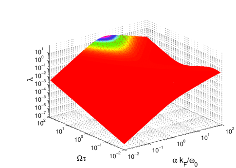
Figure 2: Gilbert damping constant as a function of SO to magnetic field ratio $\alpha k_{F}/\omega_{0}$ and disorder scale $\Omega\tau$. We assumed $n_{2D}=10^{12}cm^{-2}$ and the polarization p=0.1

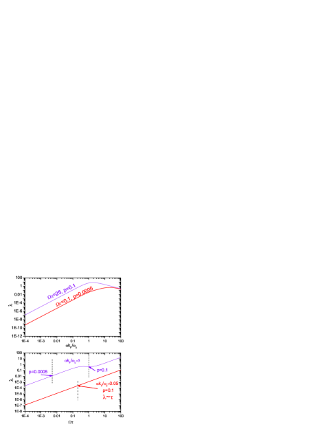
Figure 3: (a) The Gilbert damping constant as a function of SO to magnetic field ratio for two different values of disorder scale $\Omega\tau$ corresponding to the clean and dirty limits. The magnetic field and as a consequence the polarization is fixed, while the strength of spin-orbit interactions and $\tau$ changes so $\Omega\tau=$ const. The curves for $p=0.1$ and $p=0.0005$ and the ratio $\Omega\tau=0.1$ are indistinguishable. (b) The Gilbert damping as a function of disorder scale for two different values of $\alpha k_{F}/\omega_{0}$ corresponding to the strong and weak SO couplings. The magnetic field and so the polarization and the spin orbit coupling strength are fixed. The condition of validity of our calculations $E_{F}\tau\gg 1$ is on the right to the dashed line. The curves for $p=0.1$ and $p=0.0005$ and the ratio $\alpha k_{F}/\omega_{0}=5$ are indistinguishable.

The Gilbert damping constant, as given by Eq. (55) is plotted in Fig. 2 as a function of two parameters: $\Omega\tau$ – measuring the effectiveness of spin precession during an elastic mean free path $\tau$ – and $\alpha k_{F}/\omega_{0}=\bar{\alpha}/p$ the ratio of the SO effective magnetic field to the external magnetic field. Clearly $\Omega\tau\gg 1$ corresponds to the “clean” limit and $\Omega\tau\ll 1$ to the “dirty” limit.

Fig. 3 shows the two-dimensional cross-sections of Fig. 2. In Fig. 3a we see the Gilbert constant plotted as a function of the spin-orbit to polarization ratio for two values of $\Omega\tau$, one in the clean limit and one in the dirty limit. In the weak SO coupling regime ($\alpha k_{F}/\omega_{0}\ll 1$) the Gilbert constant grows as $(\alpha k_{F}/\omega_{0})^{2}$, while for strong SO coupling it saturates and begins to decrease linearly beyond a certain value $\alpha k_{F}/\omega_{0}$. The quadratic increase of $\lambda$ for small $\alpha$ is easily accounted for by the growth of the $\sin^{2}\delta$ factor in Eq. (55) – see Eq. (54). For large $\alpha$, on the other hand, $\sin\delta$ approaches the maximum value of $1$ and $\lambda$ becomes essentially proportional to $\tau$. The decrease in $\lambda$ in this regime reflects the decrease in $\tau$ along a curve on which $\Omega$ grows while $\Omega\tau$ remains constant.

Fig. 3b shows the Gilbert damping as a function of $\Omega\tau$ for two different values of $\alpha k_{F}/\omega_{0}$. For weak SO coupling (lower solid line) the Gilbert damping constant is proportional to $\tau$ in both the clean and dirty limits. This is not surprising given that in this regime the Gilbert damping is essentially proportional to the Drude conductivity. For strong SO coupling, however, we observe an interesting non-monotonic behavior of $\lambda$ (upper solid curve) in the transition region between the dirty regime ($\Omega\tau\ll 1$) and the clean one $\Omega\tau\gg 1$. This region is defined by the inequality $2\cos\delta<\Omega\tau<\sqrt{2}$, and obviously appears only if $\cos\delta$ is sufficiently small, i.e., if the SO coupling is sufficiently strong.

There is a limit, however, on how large the spin-orbit coupling can be made for a given value of $\Omega\tau$. Recall that our treatment of disorder is justified for $E_{F}\tau\gg 1$ and becomes uncontrolled when this inequality is violated. Since $E_{F}\tau=\frac{\Omega\tau}{2p\sqrt{1+(\alpha k_{F}/\omega_{0})^{2}}}$ we see that $\Omega\tau/2p$ must be larger than $\frac{\alpha k_{F}}{\omega_{0}}$ or, equivalently, $\Omega\tau>2\bar{\alpha}$ if $E_{F}\tau\gg 1$ is to be satisfied. In Fig. 3b the regions of validity of this condition, for three different values of $\bar{\alpha}$, extend to the right of the three vertical dashed lines. We see that the non-monotonic behavior for larger $\bar{\alpha}$ occurs well within the region in which our treatment of disorder is justified and can be observed if $\bar{\alpha}$ is much larger than $p$, so that $\cos\delta$ is small.

In a naive microscopic picture the Gilbert damping could be obtained by substituting the D’yakonov-Perel spin relaxation rateMishchenko et al. (2004)

$$\frac{1}{\tau_{s}}=\frac{2\tau(\alpha k_{F})^{2}}{1+(2\tau\alpha k_{F})^{2}}$$ (56)

into the phenomenological Bloch equation for spin dynamics. This results in the formula

$$\lambda\sim\frac{\tau_{s}}{1+(\omega_{0}\tau_{s})^{2}}\,.$$ (57)

which reproduces Eq. (55) either in the weak-SO limit with $\alpha k_{F}\ll 1/\tau,\omega_{0}$ or in the absence of the applied field, $\omega_{0}=0$, where Eq. (56) becomes the correct Bloch spin relaxation rate of the unpolarized Rashba 2DEG Mishchenko et al. (2004). We note, however, that the full structure of Eq. (55) cannot be completely captured by the D’yakonov-Perel spin relaxation rate (56). In particular in the clean limit the combined Eqs. (56) – (57) would lead to the scaling of $\lambda$ as $1/\tau$, which tends to zero, while our Eq. (55) gives scaling of $\lambda$ as $\tau$, which tends to infinity.

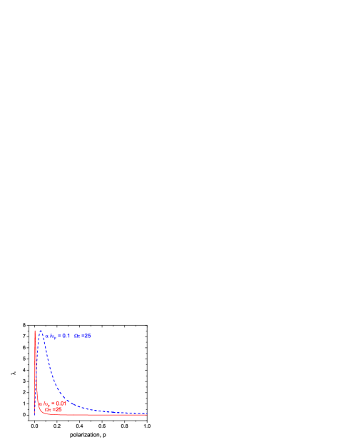
Figure 4: The Gilbert damping constant as a function of polarization for two different values of renormalized spin-orbit coupling $\bar{\alpha}=\alpha/\upsilon_{F}$.

Fig. 4 shows the Gilbert damping as a function of polarization for two different values of spin-orbit coupling. One can see that Gilbert damping increases with $p$ for $p<\bar{\alpha}$ and decreases with further increase of $p$ above $\bar{\alpha}$. Tunable magnetization damping is very desirable since it allows to reduce post-switching magnetization precession S. Ingvarsson and Koch . Fig. 4 shows the possibility of tuning of the Gilbert damping by changing temperature in a polarized 2DEG with spin-orbit interactions.

The $\omega$ dependent spin-channel conductivity, can be obtained through the replacement of $\frac{1}{\tau}$ by $\frac{1}{\tau}-i\omega$ (see also appendix A) and has a form:

$$\Re e\sigma_{s\parallel}(\omega)=\sigma_{D}\frac{\cos^{2}\delta}{1+(\omega\tau)^{2}}$$

$$\times \frac{1+(\Omega\tau)^{2}[\frac{1}{2}\sin^{2}\delta+(\cos\delta+\omega/\Omega)^{2}]}{\cos^{2}\delta+(\Omega\tau)^{2}[\frac{1}{2}\sin^{2}\delta+\cos\delta(\cos\delta+\omega/\Omega)]^{2}}~{},$$

which gives

$$\lambda_{ni}(\omega)=p\frac{\bar{\alpha}^{2}E_{F}\tau}{\hbar(p^{2}+\bar{\alpha}^{2})}\frac{1}{1+(\omega\tau)^{2}}$$

$$\times \frac{1+(\Omega\tau)^{2}[\frac{1}{2}\sin^{2}\delta+(\cos\delta+\omega/\Omega)^{2}]}{\cos^{2}\delta+(\Omega\tau)^{2}[\frac{1}{2}\sin^{2}\delta+\cos\delta(\cos\delta+\omega/\Omega)]^{2}}~{}.$$

These equations reduce to Eqs. (51) and (55) respectively if we set $\omega=0$.

Notice the very different limiting behavior of $\lambda$ as a function of the disorder strength for $\omega=0$ and $\omega$ finite. In the first case, $\lambda$ tends to infinity as the scattering time $\tau$ increases (i.e. for decreasing disorder). At finite $\omega$ however, the Gilbert constant goes to zero for $\tau$ tending to infinity. This is the proper “clean limit”. In the opposite limit of strong disorder, the Gilbert damping decreases monotonically to zero. This is a manifestation of the D’yakonov-Perel effect: in a strongly disordered system the instantaneous axis of spin-precession changes too rapidly to allow an effective loss of spin orientation.

Instead of using the equation of motion to calculate the Gilbert damping, we could evaluate directly the imaginary part of the transverse spin response function. The two approaches are equivalent and the details of the calculations of the transverse spin response function are summarized in Appendix D. We will see in the following, however, that the treatment in terms of the spin-channel conductivities allow us to gain useful intuition for the inclusion of $e-e$ interaction effects.

IV.1.2 Interacting 2DEG

The role of the Coulomb interaction in spin transport was analyzed in detail in Refs. D’Amico and Vignale, 2000, 2002, but only in the absence of SO coupling. In the spin-polarized electron liquid, with identical scattering times for up and down spins and $\alpha=0$ the result is

$$\Re e\sigma_{s\parallel}(0)=\sigma_{D}\frac{1+p^{2}\gamma\tau}{1+\gamma\tau}~{},$$ (60)

where $\gamma$ is the spin-drag coefficient – the rate of momentum transfer due to the Coulomb interaction between up and down spins. The derivation of Eq. (60) is presented for completeness in Appendix B.

Notice that the effect of the spin Coulomb drag vanishes (as expected) when the electron gas is fully spin polarized, i.e. when $p=1$. This is because in this limit there are no minority spin carriers to exert a drag on the majority spin carriers. More generally, the form of Eq. (60) can be understood in terms of the coupling between charge and spin currents in a spin-polarized electron gas. A “spin electric field” $E_{s}=E_{\uparrow}=-E_{\downarrow}$ drives not only a spin current, but also a charge current $j_{c}=p\sigma_{D}E_{s}$ (notice that $\gamma$ does not enter here). The charge-current acts on the spin current as an additional spin electric field $\frac{m\gamma}{ne^{2}}pj_{c}=\gamma\tau p^{2}E_{s}$. The spin current then responds in the usual way (i.e. with the unpolarized spin conductivity $\sigma_{s}|_{p=0}=\frac{\sigma_{D}}{1+\gamma\tau}$) to an enhanced spin electric field $E_{s}(1+\gamma p^{2}\tau)$. This gives Eq. (60).

The low-temperature behavior of $\gamma$ is approximately given by the formula

$$\gamma(T) = \frac{E_{F}}{\hbar}\left(\frac{k_{B}T}{E_{F}}\right)^{2}\frac{\pi r_{s}^{2}}{6(1-p^{2})^{3/2}}$$

$$\times \int_{0}^{1}\frac{dx}{{(\sqrt{x}+\frac{r_{s}}{\sqrt{2(1-p)}})^{2}}\sqrt{1-x}\sqrt{1-ax}}~{},$$

where $a=(1-p)/(1+p)$. For zero polarization, $\gamma$ diverges logarithmically as can be easily by putting $p=0$ under integral in Eq. (IV.1.2). Thus $\gamma$ scales quadratically with temperature for $T/T_{F}\ll 1$, but has a non-monotonic behavior as a function of polarization.

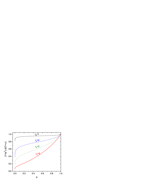
Figure 5: The behavior of renormalization factor $(1+p^{2}\gamma\tau)/(1+\gamma\tau)$ associated with electron-electron interactions as a function of polarization for various $r_{s}$.

The behavior of the spin conductivity renormalization factor $(1+p^{2}\gamma\tau)/(1+\gamma\tau)$ of Eq. (60) is shown in Fig. 5 as a function of $p$ for several values of $r_{s}$, assuming $E_{F}\tau/\hbar=10/r_{s}^{2}$ and $k_{B}T/E_{F}=r_{s}^{2}/10$. We see that the reduction of the spin conductivity and hence of $\lambda$ due to Coulomb interaction is significant for small and intermediate polarizations, especially at larger values of $r_{s}$.

The calculation of the spin drag coefficient in the presence of SO coupling poses, of course, a more difficult problem. However, in view of the fact that the SO energy scale is usually much smaller than the Coulomb energy scale such a detailed calculation is not urgently needed. Coulomb interaction corrections are adequately taken into account by multiplying the non-interacting result of Eq. (55) by the correction factor on the right hand side of E. (60). This gives

$$\lambda=\lambda_{ni}\frac{1+p^{2}\gamma\tau}{1+\gamma\tau}~{}.$$ (62)

Eq. (62) has the interesting property that it scales as $\tau$ for $\gamma p^{2}\tau\gg 1$ and $\gamma\tau\gg 1$ as well as in opposite limit when $\gamma p^{2}\tau\ll 1$ and $\gamma\tau\ll 1$. The $e-e$ interactions plays a role mostly in the regime $1\ll\gamma\tau\ll 1/p^{2}$ which shrinks to zero as $p$ increases. The behavior of Gilbert constant as a function of $\gamma\tau$ and polarization $p$ is presented in Fig. 6 and Fig. 7. For strong polarization the factor $(1+p^{2}\gamma\tau)/(1+\gamma\tau)\sim 1$ and the Gilbert damping scales with a scattering time $\tau$. The situation looks different for a very weak polarization (see solid line in Fig. 7): the Gilbert damping scales as $\tau/(1+\gamma\tau)$ for a weak $e-e$ interactions but for strong $e-e$ interactions it saturates to a constant value proportional to $1/\gamma$.

The dependence of $\lambda$ on polarization is more complicated. This is a consequence of the fact that the spin-Coulomb drag depends on polarization. For weak $e-e$ interaction $\lambda$ increases linearly with $p$ for small $p$ and saturates for large $p$. For strong $e-e$ interactions ($\gamma\tau>1$) $\lambda$ increases linearly with $p$ for small $p$, and increases even faster than $p$ for strong polarization.

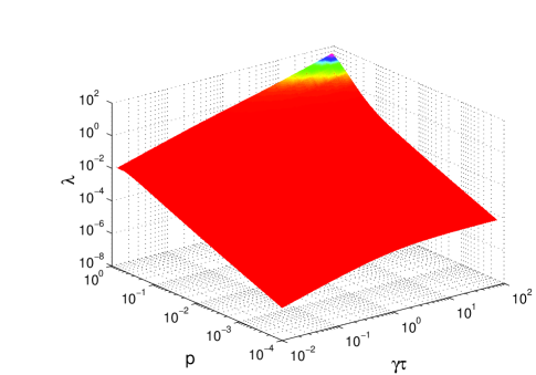
Figure 6: Gilbert damping constant as a function of $\gamma\tau$ and polarizatioon p for $n_{2D}=10^{12}cm^{-2}$ and $m_{eff}=0.067m_{e}$. We chose the limit of weak spin orbit coupling $\alpha k_{F}/\omega_{0}=0.02$ and $T/T_{F}=0.02$.

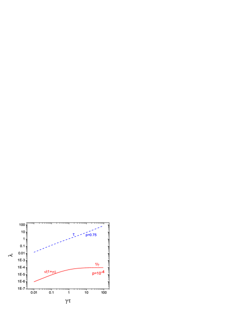
Figure 7: The Gilbert damping constant as a function $\gamma\tau$, the two-dimensional cross-section through the 3D plot presented in Fig.5.

It is also possible to include the frequency dependence of the spin Coulomb drag correction through the replacement of $\frac{1}{\tau}$ by $\frac{1}{\tau}-i\omega$. A straightforward calculation gives

$$\lambda(\omega)=\lambda_{ni}(\omega)\frac{(1+\gamma\tau)(1+p^{2}\gamma\tau)+(\omega\tau)^{2}}{(1+\gamma\tau)^{2}+(\omega\tau)^{2}}~{}.$$ (63)

IV.2 Anisotropic case

Let us now consider the general anisotropic case, in which the direction ${\bf\hat{e}_{3}}$ of the magnetization forms an angle $\Theta$ with the direction ${\bf\hat{e}_{z}}$ of the electric field that generates the SO effective magnetic field. An exact calculation of the torque-torque response function is complicated, even in the noninteracting case, by the lack of rotational symmetry about the ${\bf\hat{e}_{3}}$ axis. However, in the limit of small $\alpha$, the spin degrees of freedom are decoupled from the orbital degrees of freedom and we can take advantage of rotational symmetry about the ${\bf\hat{e}_{3}}$ axis in spin space to simplify the calculation. What happens is that response functions such as $\langle\langle\sum_{n}\hat{S}_{n3}\hat{p}_{nx};\sum_{n}\hat{S}_{n\perp}\hat{p}_{nx}\rangle\rangle_{\omega}$ vanish by symmetry when $\hat{S}_{\perp}$ denotes one of the two transverse components, $\hat{S}_{1}$ or $\hat{S}_{2}$, of the spin operator. On the other hand, the response function $\langle\langle\sum_{n}\hat{S}_{n\perp}\hat{p}_{nx};\sum_{n}\hat{S}_{n\perp}\hat{p}_{nx}\rangle\rangle_{\omega}$ does not depend on which component $\hat{S}_{n\perp}$ we choose to consider.

Going back to Eqs. (32-33) and making use of Eq. (41) we see that, to second order in $\bar{\alpha}$ we have

$$\lambda_{1}=\frac{\bar{\alpha}^{2}E_{F}\tau}{\hbar p}\left[\frac{\Re e\sigma_{s\parallel}(0)}{\sigma_{D}}+\sin^{2}\Theta\frac{\Re e\sigma_{s\perp}(0)}{\sigma_{D}}\right]~{},$$ (64)

and

$$\lambda_{2}=\frac{\bar{\alpha}^{2}E_{F}\tau}{\hbar p}\left[\cos^{2}\Theta\frac{\Re e\sigma_{s\parallel}(0)}{\sigma_{D}}+\sin^{2}\Theta\frac{\Re e\sigma_{s\perp}(0)}{\sigma_{D}}\right]~{},$$ (65)

where the transverse spin-channel conductivity $\sigma_{s\perp}$ is defined, in analogy to Eq. (44) as

$$\Re e\sigma_{s\perp}(\omega)=-\frac{4e^{2}}{m^{2}{\cal V}}\Im m\frac{\langle\langle\sum_{n}\hat{S}_{n\perp}\hat{p}_{nx};\sum_{n}\hat{S}_{n\perp}\hat{p}_{nx}\rangle\rangle_{\omega}}{\hbar^{2}\omega}~{}.$$ (66)

The calculation of $\sigma_{s\perp}$ in the absence of SO coupling and $e-e$ interactions is straightforward and yields

$$\Re e\sigma_{s\perp}(0)=\frac{\sigma_{D}}{1+(\omega_{0}\tau)^{2}}$$ (67)

Notice that this differs from the longitudinal spin-channel conductivity $\sigma_{s\parallel}$, calculated in the same approximation, simply by the factor $[1+(\omega_{0}\tau)^{2}]^{-1}$. This takes into account the non-conservation (precession) of the transverse spin caused by the magnetic field in the ${\bf\hat{e}_{3}}$ direction. Therefore, in the limit of weak SO coupling and no interaction we get

$$\lambda_{1}=\frac{\bar{\alpha}^{2}E_{F}\tau}{\hbar p}\left[1+\frac{\sin^{2}\Theta}{1+(\omega_{0}\tau)^{2}}\right]~{},$$ (68)

and

$$\lambda_{2}=\frac{\bar{\alpha}^{2}E_{F}\tau}{\hbar p}\left[\cos^{2}\Theta+\frac{\sin^{2}\Theta}{1+(\omega_{0}\tau)^{2}}\right]~{}.$$ (69)

The effect of the spin Coulomb drag can be included, at the same level of approximation, by multiplying the two spin-channel conductivities by appropriate renormalization factors. Namely, we use Eq. (60) for $\sigma_{s\parallel}(0)$, and

$$\Re e\sigma_{s\bot}(0)=\sigma_{D}\frac{1+\gamma_{\bot}\tau}{(\omega_{0}\tau)^{2}+(1+\gamma_{\bot}\tau)^{2}}~{},$$ (70)

where $\gamma_{\perp}$ is a transverse-spin analogue of the longitudinal spin Coulomb drag coefficient, as discussed in Appendix C.

An unsatisfactory feature of Eqs. (68) and  (69) is that they are valid only for $\alpha k_{F}\ll\omega_{0}$. Notice however that the angular dependence of the Gilbert constants in these equations reduces to simple angular factors multiplying the isotropic result. This suggests that we take care of the problem simply by multiplying the full isotropic non-interacting result for $\lambda(\omega)$, given by Eq. (55), by the same angular factor. The resulting expressions:

$$\lambda_{1}=\lambda_{ni}\left[\frac{\Re e\sigma_{s\parallel}(0)}{\sigma_{D}}+\sin^{2}\Theta\frac{\Re e\sigma_{s\perp}(0)}{\sigma_{D}}\right]~{},$$ (71)

and

$$\lambda_{2}=\lambda_{ni}\left[\cos^{2}\Theta\frac{\Re e\sigma_{s\parallel}(0)}{\sigma_{D}}+\sin^{2}\Theta\frac{\Re e\sigma_{s\perp}(0)}{\sigma_{D}}\right]~{},$$ (72)

with $\lambda_{ni}$, $\Re e\sigma_{s\parallel}(0)$ and $\Re e\sigma_{s\perp}(0)$ given by Eqs. (55), (60) and (70) respectively, vanish for $\omega_{0}$ tending to zero, and should be reasonable not only for $\alpha k_{F}\ll\omega_{0}$ but also for $\alpha k_{F}\gg\omega_{0}$ provide both energies are small compared to the Fermi energy. Furthermore these formulas can be generalized to finite frequency simply replacing $\lambda_{ni}$ by $\lambda_{ni}(\omega)$ (Eq. (IV.1.1)) and replacing $\frac{1}{\tau}$ by $\frac{1}{\tau}-i\omega$ in the Coulomb renormalization factors.

V Generalizations and conclusion

In this paper we have shown that (1) the Gilbert damping constant for a homogenously magnetized electron gas with SO interactions can be exactly expressed in terms of the torque-torque correlator which comes from SO interactions; (2) In the special case of the Rashba model the Gilbert damping can be expressed in terms of the spin-channel conductivity. Based on this connection, we have discussed the behavior of the Gilbert damping constant in a two-dimensional electron gas with Rashba SO coupling as a function of magnetic field, SO interaction, $e-e$ interaction, and disorder. These calculations, while based on linear response theory, do nevertheless provide the input for the nonlinear LLG equation, provided it is recognized that $\stackrel{{\scriptstyle\leftrightarrow}}{{\lambda}}$ depends on the instantaneous orientation of the magnetization.

It should be clear that point (1) above is completely general, while point (2) depends on a specific feature of the Rashba spin-orbit interaction, namely, the fact that the electric field is independent of position. This poses the question: to what extent is the connection between Gilbert damping and spin conductivity transferrable to general, non-homogeneous, spin-orbit coupled systems?

In this conclusion we argue that the connection is indeed broadly applicable to itinerant-electron ferromagnets, under assumptions similar to those that are used to justify the local density approximation (LDA) in the density functional theory of electronic structure. We recall that in a multi-band all-electrons theory the SO interaction has the form:

$$\hat{H}_{SO}=-\frac{1}{2m^{2}c^{2}}\sum_{n}\left(\hat{\nabla}V({\bf r}_{n})\times\hat{\bf p}_{n}\right)\cdot{\bf\hat{S}}_{n}~{}$$ (73)

where $V({\bf r})$ is the self-consistent Kohn-Sham potential, typically given by the local density approximation. The gradient of $V({\bf r})$ defines a privileged direction at each point in space, which we denote ${\bf\hat{e}_{z}}({\bf r})$. Then the spin-orbit interaction can be recast in the form

$$\hat{H}_{SO}=-\sum_{n}\frac{\alpha({\bf r}_{n})}{\hbar}\left[{\bf\hat{e}_{z}}({\bf r}_{n})\times\hat{\bf p}_{n}\right]\cdot{\bf\hat{S}}_{n}~{},$$ (74)

where $\alpha({\bf r})$ is a position dependent SO coupling constant, which reflects the local magnitude of the electric field seen by the electron, and ${\bf\hat{e}_{z}}({\bf r})$ is the local direction of this field. Another privileged direction is the direction of the local magnetization, which we call ${\bf\hat{e}_{3}}({\bf r})$. Thus we are back to our model hamiltonian (38) (we already remarked that the two-dimensionality of the model is not essential to our treatment) with the crucial difference that $\alpha,{\bf\hat{e}_{z}}$, and ${\bf\hat{e}_{3}}$ are functions of position.

Now in the spirit of the LDA let us assume that the Kohn-Sham potential, its gradient, and the direction of the magnetization are all slowly varying on the appropriate microscopic length scale (e.g., the electron-electron distance, or the size of the unit cell, or the scattering mean free path). Then we can equiparate each small volume element of the system to a homogeneously magnetized electron gas of density $n$ and polarization $p$ pointing in the ${\bf\hat{e}_{3}}$ direction, with a SO coupling constant $\alpha({\bf r})$ and a local anisotropy axis ${\bf\hat{e}_{z}}$. With this identification, all the results obtained in the previous section become immediately applicable to each volume element.

An obvious objection to this procedure is that the electronic density of real materials is not slowly varying on the atomic scale. In spite of this, however, it is well known that the LDA works very well in materials because the exchange correlation potential is controlled by a spherical average of the exchange-correlation hole, which is reasonably close to the spherical hole of the homogeneous electron gas. We believe that a similar averaging may also work for the magnetization dynamics. Then the Gilbert damping would be given by the formulas derived in this paper, only with the appropriate coarse-grained values of $\alpha,{\bf\hat{e}_{z}}$, and ${\bf\hat{e}_{3}}$.

VI Acknowledgements

We thank Allan H. MacDonald and Arne Brataas for enlightening discussions. This work was supported by NSF Grant No. DMR-0313681 and supported in part by the National Science Foundation under Grant No. PHY99-07949.

VII Appendix A: Longitudinal spin-channel conductivity for noninteracting electrons

In the calculations that follow we set $\hbar=1$ for convenience. To obtain the real part of longitudinal spin-channel conductivity we need to calculate $\Im m\frac{\langle\langle\sum_{n}\hat{S}_{n3}\hat{p}_{nx};\sum_{n}\hat{S}_{n3}\hat{p}_{nx}\rangle\rangle_{\omega}}{\omega}$. For a magnetization parallel to the $z$ axis (i.e. $\Theta=0$) the above expression simplifies to $\Im m\frac{\langle\langle\hat{S}_{z}\hat{P}_{x};\hat{S}_{z}\hat{P}_{x}\rangle\rangle_{\omega}}{\omega}$ where $\hat{S}_{z}$ is the $z$ component of the spin operator and $\hat{P}_{x}$ is $x$ component of the total momentum. For non-zero $\omega$ we have to evaluate the following integral:

$$\Im m\frac{\langle\langle\hat{S}_{z}\hat{P}_{x};\hat{S}_{z}\hat{P}_{x}\rangle\rangle_{\omega}}{\omega{\cal V}}=\frac{1}{\omega}\Im m\left\{\int\frac{d\epsilon}{2\pi i}\int\frac{d^{2}p}{(2\pi)^{2}}p_{x}Tr[\hat{S}_{z}\hat{G}(p,\epsilon+\omega)\hat{\Lambda}_{x}(\epsilon)\hat{G}(p,\epsilon)]\right\}\\$$

where

$$G(p,\omega)=\frac{1}{\omega-\epsilon_{p}-\vec{h}_{p}\vec{S}+i/2\tau_{\omega}}$$ (75)

is the disorder-averaged Green’s function near the Fermi level, $\epsilon_{p}$ is the kinetic energy relative to the Fermi level, $\vec{h}_{p}=(\alpha p_{y},-\alpha p_{x},\omega_{0})$ is the effective magnetic field, $\vec{S}=\vec{\sigma}/2$,where $\vec{\sigma}$ is the vector of Pauli matrices and

$$\frac{1}{\tau_{\omega}}\equiv\frac{1}{\tau}{\rm sign}(\omega)~{}.$$ (76)

Using the fact that the integration over energy involves only the states around the Fermi energy, i.e. $\epsilon+\omega>E_{F}$ and $\epsilon<E_{F}$ allows us to integrate over $\epsilon$ and cancel out the $1/\omega$ on the r.h.s. of Eq. (VII). Then one can see that the formula for a non-zero $\omega$ can be obtained from the $\omega=0$ limit with the substituition $1/\tau\to 1/\tau-i\omega$, leading to Eq. (IV.1.1).

In the $\omega=0$ limit $\hat{G}(\epsilon+\omega)$ and $\hat{G}(\omega)$ should be substituted by $\hat{G}(0^{+})$ and $\hat{G}(0^{-})$, respectively. The ladder vertex corrections are found by solving the self-consistent integral equation for $\hat{\Lambda}$. For an electron-impurity potential of the form $U\delta({\bf r})$ this equation is

$$\vec{\Lambda}=\vec{p}S_{z}+U^{2}\int\frac{d^{2}p^{\prime}}{(2\pi)^{2}}\hat{G}(p^{\prime},0^{+})\vec{\Lambda}\hat{G}(p^{\prime},0^{-})$$ (77)

Its solution gives the vertex correction of the following form:

$$\Lambda_{x}=p_{x}S_{z}+\frac{\alpha p_{F}^{2}}{2}\left(\frac{i\omega_{0}-1/\tau}{\Omega^{2}+\omega_{0}^{2}+2i\omega_{0}/\tau}S_{+}+h.c.\right)$$ (78)

where $S_{+}=S_{x}+iS_{y}$ and $U^{2}=1/m\tau$.

The calculation of the spin-channel conductivity in Eq. (VII) without the vertex corrections (a single bubble) gives:

$$\Im m\frac{\langle\langle\hat{S}_{z}\hat{P}_{x};\hat{S}_{z}\hat{P}_{x}\rangle\rangle_{\omega}}{\omega{\cal V}}=-\frac{mn\tau}{4}\left(\frac{\Omega^{2}\tau^{2}cos\delta+1}{\Omega^{2}\tau^{2}+1}\right)$$ (79)

while the final result including the ladder vertex corrections is:

$$\Im m\frac{\langle\langle\hat{S}_{z}\hat{P}_{x};\hat{S}_{z}\hat{P}_{x}\rangle\rangle_{\omega}}{\omega{\cal V}}=\frac{-mn\tau}{4}\frac{\cos^{2}\delta\left[1+\frac{1}{2}\Omega^{2}\tau^{2}(1+\cos^{2}\delta)\right]}{\cos^{2}\delta+\frac{1}{4}\Omega^{2}\tau^{2}(1+\cos^{2}\delta)^{2}}$$

Using Eq. (VII), and the definition of spin channel conductivity we finally obtain the formula Eq. (51) for the real part of longitudinal spin-channel conductivity:

$$\Re e\sigma_{s\parallel}(0)=\sigma_{D}\cos^{2}\delta\frac{1+\frac{1}{2}(\Omega\tau)^{2}(1+\cos^{2}\delta)}{\cos^{2}\delta+\frac{1}{4}(\Omega\tau)^{2}(1+\cos^{2}\delta)^{2}}~{}$$

The single bubble calculation recovers the behavior of the longitudinal spin-conductivity for weak SO interactions: Eqs. (79) and (VII) coincide for $\delta=0$, i.e. fora zero SO coupling. However, for strong spin-orbit interactions the vertex corrections are absolutely necessary. Moreover, only Eq. (VII) gives the correct result for zero magnetic field, i.e. $\Re e\sigma_{s\parallel}(0)=0$.

VIII Appendix B: Longitudinal spin-channel conductivity in the presence of $e-e$ interactions

In the absence of SO interactions the structure of the $2\times 2$ resistivity matrix can be deduced from the equation of motion for electrons with spin $\sigma$ and velocity $\upsilon_{\sigma}$:

$$m^{*}N_{\sigma}\vec{\dot{\upsilon}}_{\sigma}=-eN_{\sigma}\vec{E}_{\sigma}+\vec{F}^{C}_{\sigma\bar{\sigma}}-\frac{m^{*}}{\tau_{\sigma}}N_{\sigma}\vec{\upsilon}_{\sigma}$$ (81)

where $m^{*}$ is the effective mass of the electrons, $\bar{\sigma}\equiv-\sigma$, $F^{C}_{\sigma\bar{\sigma}}$ is the average Coulomb force between electrons of opposite spin orientations, which is proportional to the difference of their drift velocities. The Fourier transformation of Eq. (81) leads to the following formula for the spin current:

$$i\omega\vec{j}_{\sigma}=\frac{-n_{\sigma}e^{2}}{m^{*}}\vec{E}_{\sigma}(\omega)+\left(\frac{n_{\bar{\sigma}}}{n}\gamma+\frac{1}{\tau_{\sigma}}\right)\vec{j}_{\sigma}(\omega)-\frac{n_{\sigma}}{n}\gamma\vec{j}_{\bar{\sigma}}(\omega)~{}.$$

Using Eq. (VIII), we can show that the resistivity tensor has the form:

$$\rho=\begin{pmatrix}\frac{m^{*}}{n_{\uparrow}e^{2}}\left(-i\omega+\frac{1}{\tau_{\uparrow}}+\frac{n_{\downarrow}}{n}\gamma\right)&-\frac{m^{*}}{ne^{2}}\gamma\\ -\frac{m^{*}}{ne^{2}}\gamma&\frac{m^{*}}{n_{\downarrow}e^{2}}\left(-i\omega+\frac{1}{\tau_{\downarrow}}+\frac{n_{\uparrow}}{n}\gamma\right)\end{pmatrix}$$ (83)

Inverting the resistivity matrix we get the following formula for the spin-channel conductivity $\sigma_{s{\|}}$:

$$\sigma_{s\|}(\omega)=\frac{\rho_{\downarrow\downarrow}+\rho_{\uparrow\uparrow}+\rho_{\uparrow\downarrow}+\rho_{\downarrow\uparrow}}{\rho_{\uparrow\uparrow}\rho_{\downarrow\downarrow}-\rho_{\uparrow\downarrow}\rho_{\downarrow\uparrow}}$$ (84)

Substituting the elements of the resistivity matrix into Eq. (84) one obtains:

$$\sigma_{s\|}(\omega)=\sigma_{D}\frac{[\omega^{2}+1/\tau^{2}(1+\gamma\tau p^{2})](\gamma+1/\tau)-\gamma p^{2}\omega^{2}}{(\omega^{2}\tau+1/\tau)[\omega^{2}+(1/\tau+\gamma)^{2}]}$$ (85)

If $\omega=0$, Eq. (85) simplifies to Eq. (60):

$$\Re e\sigma_{s\parallel}(0)=\sigma_{D}\frac{1+p^{2}\gamma\tau}{1+\gamma\tau}~{},$$

For zero polarization the spin and charge channels are decoupled and the inverse of the effective scattering time consists of two contributions, one connected with disorder and second one associated with e-e interactions:

$$\tau^{-1}_{eff}=\tau^{-1}+\gamma$$ (86)

For nonzero polarization the spin and charge channels are mixed and the additional term $\gamma p^{2}\tau$ appears in the numerator.

IX Appendix C: Transverse spin-channel conductivity in the presence of $e-e$ interactions

In this appendix we use the semi-classical approach (similar to the one presented in a previous appendix) to calculate the real part of the transverse spin-channel conductivity. According to Eq. (66):

$$\Re e\sigma_{xx}=\Re e\sigma_{\bot}=-\frac{4e^{2}}{m^{2}{\cal V}}\Im m\frac{\langle\langle\sum_{n}\hat{S}_{nx}\hat{p}_{nx};\sum_{n}\hat{S}_{nx}\hat{p}_{nx}\rangle\rangle_{\omega}}{\hbar^{2}\omega}$$

so we are looking for a spin current response on the perturbation $p_{x}S_{x}$. This perturbation is generated by the SU(2) vector potential $A_{x}S_{x}$ where $S_{x}$ is the $x$-component of the spin operator. As a consequence one can show that the “electric field” that drives the change of spin current does not depend on spin (see Eq. (87) below). We neglect SO interactions in this calculation and work in the circularly polarized basis in which the spin-conductivity is diagonal and has two components $\sigma_{s}^{+}(\omega)$ and $\sigma_{s}^{-}(\omega)$. The diagonal character of the conductivity in this basis is equivalent to the statement that the current of right-handed circularly polarized electrons, $j_{+}$ does not interact with the current of left-handed circularly polarized electrons $j_{-}$. The semiclassical equation of motion for these currents is

$$\frac{e}{V}\sum_{i}\frac{d}{dt}(S_{i\pm}{\upsilon}_{ix})=-\sum_{i}\frac{e^{2}E}{m^{*}}-\sum_{i}\frac{eS_{i\pm}\upsilon_{ix}}{\tau}-\sum_{i}eS_{i\pm}\upsilon_{ix}\gamma_{\bot}$$ (87)

where $S_{\pm}=S_{x}\pm iS_{y}$, $\upsilon_{x}$ is the $x$-component of the velocity and $\gamma_{\bot}$ is in plane spin-Coulomb drag coefficient. The Fourier transformation of Eq. (87) leads to the following formula for the left and right circularly polarized spin current densities:

$$i(\omega\pm\omega_{0})j_{\pm}=-ne^{2}\frac{E}{m^{*}}+\frac{j_{\pm}}{\tau}+j_{\pm}\gamma_{\bot}$$ (88)

where we used the fact that in the absence of SO coupling:

$$\frac{dS_{\pm}}{dt}=-i[S_{\pm},\hat{H}]=\pm i\omega_{0}S_{\pm}$$ (89)

Then the circularly polarized spin conductivities have the form:

$$\sigma_{\pm}=\frac{ne^{2}}{m^{*}}\frac{1}{-(\omega\pm\omega_{0})i+\frac{1}{\tau}+\gamma_{\bot}}$$ (90)

where we assumed that the spin-Coulomb drag coefficient is the same for both circular polarizations. Accordingly, the real parts of spin conductivities have the following form:

$$\Re e\sigma^{s}_{\pm}(\omega)=\frac{ne^{2}}{m^{*}}\frac{\gamma_{\bot}+1/\tau}{(\omega\mp\omega_{0})^{2}+(\gamma_{\bot}+1/\tau)^{2}}$$ (91)

Assuming that $\omega\gg 1/\tau,\gamma,\omega_{0}$ we find the real part of the transverse spin channel conductivity $\sigma^{s}_{\bot}(\omega)$ as follows: Eq. (91):

$$\Re e\sigma^{s}_{\bot}(\omega)=\frac{\Re e\sigma^{s}_{+}(\omega)+\Re e\sigma^{s}_{-}(\omega)}{4}=\frac{ne^{2}}{2m^{*}}\frac{\gamma_{\bot}+1/\tau}{\omega^{2}}~{}.$$ (92)

Eq. (92) separates the disorder and interaction terms. Since we have already included disorder in the phenomenological Eq. (88), it is justified to derive the transverse spin-drag coefficient $\gamma_{\bot}$ by comparing Eq. (92) with the transverse spin-channel conductivity found from Eq. (66). Using two times the identity (19) we can rewrite Eq. (66) in terms of the force-force correlation function:

$$Re\sigma_{\bot}(\omega)=-\frac{4e^{2}}{m^{2}{\cal V}}\Im m\frac{\langle\langle\sum_{n}\hat{S}_{nx}\hat{F}_{nx};\sum_{n}\hat{S}_{nx}\hat{F}_{nx}\rangle\rangle_{\omega}}{\omega^{3}}$$ (93)

Then by comparing Eq. (92) with Eq. (93) we obtain in the clean limit:

$$\gamma_{\bot}(\omega)=-\frac{8}{nm^{*}{\cal V}}\Im m\frac{\langle\langle\sum_{n}\hat{S}_{nx}\hat{F}_{nx};\sum_{n}\hat{S}_{nx}\hat{F}_{nx}\rangle\rangle_{\omega}}{\omega}=$$

$$\frac{1}{2\pi^{2}nm^{*}}\int_{0}^{\infty}dqq^{3}\nu^{2}_{q}\frac{e^{-\beta\omega}-1}{\omega}\int_{0}^{\omega}d\omega^{\prime}\frac{\Im m\chi_{nn}(q,\omega^{\prime})\Im m\chi_{xx}(q,\omega-\omega^{\prime})}{(e^{-\beta\omega^{\prime}}-1)(e^{-\beta(\omega-\omega^{\prime})}-1)}=$$

$$\frac{k_{F}^{4}}{2\pi^{2}nm^{*}}\int_{0}^{\infty}d\bar{q}\bar{q}^{3}\nu^{2}_{\bar{q}}\int_{0}^{\bar{\omega}}\frac{e^{-2\beta E_{F}\bar{\bar{\omega}}}-1}{\bar{\omega}}d\bar{\omega}^{\prime}\frac{\Im m\chi_{nn}(\bar{q},\bar{\omega}^{\prime})\Im m\chi_{xx}(\bar{q},\bar{\omega}-\bar{\omega}^{\prime})}{(e^{-2\beta E_{F}\bar{\omega}^{\prime}}-1)(e^{-2\beta E_{F}(\bar{\omega}-\bar{\omega}^{\prime})}-1)}$$ (94)

where $\bar{q}=q/k_{F}$, $\bar{\omega}=\hbar\omega/2E_{F}$. For small $\bar{\omega}$

$$\nu_{\bar{q}}\Im m\chi_{xx}(\bar{q},\bar{\omega})=-\frac{1}{\sqrt{2}}\frac{\bar{\omega}/\bar{q}}{\sqrt{1-\frac{p^{2}}{\bar{q}^{2}}-\frac{\bar{q}^{2}}{4}}}\frac{r_{s}}{\bar{q}+r_{s}\sqrt{2}}$$ (95)

and $\Im m\chi_{nn}(\bar{q},\bar{\omega})=\Im m\chi_{\uparrow}(\bar{q},\bar{\omega})+\Im m\chi_{\downarrow}(\bar{q},\bar{\omega})$, where

$$\nu_{\bar{q}}\Im m\chi_{\uparrow}(\bar{q},\bar{\omega})=-\frac{1}{\sqrt{2}}\frac{\bar{\omega}/\bar{q}}{\sqrt{1+p-\frac{\bar{q}^{2}}{4}}}\frac{r_{s}}{\bar{q}+r_{s}\sqrt{2}}$$ (96)

and $\Im m\chi_{\downarrow}(\bar{q},\bar{\omega})$ is obtained from the above equation simply by changing the sign of $p$. $\nu_{\bar{q}}$ is the dimensionless screened interaction potential and $r_{s}=\frac{1}{\sqrt{\pi n}a_{B}}$ is the dimensionless Wigner-Seitz radius. In the limit of $T/T_{F}\ll 1$ this formula can be evaluated analytically leading to the following integral on the transverse spin Coulomb drag coefficient:

$$\gamma_{\bot}(0)=\frac{E_{F}}{\hbar}\left(\frac{k_{B}T}{E_{F}}\right)^{2}\frac{\pi r_{s}^{2}}{6}\left[F(r_{s},p)+F(r_{s},-p)\right]$$ (97)

where

$$F(r_{s},p)=\int_{a(p)}^{b(p)}\frac{\bar{q}d\bar{q}}{(\bar{q}+\sqrt{2}r_{s})^{2}}\frac{1}{\sqrt{\left(1-\frac{p^{2}}{\bar{q}^{2}}-\frac{\bar{q}^{2}}{4}\right)\left(1+p-\frac{\bar{q}^{2}}{4}\right)}}~{},$$ (98)

for $b(p)\geq a(p)$ and zero otherwise, and the limits of integration are

$$a(p)\equiv|\sqrt{1+p}-\sqrt{1-p}|~{},~{}~{}~{}~{}~{}~{}~{}~{}~{}b(p)\equiv{\rm min}(\sqrt{1+p}+\sqrt{1-p},2\sqrt{1+p})~{}.$$ (99)

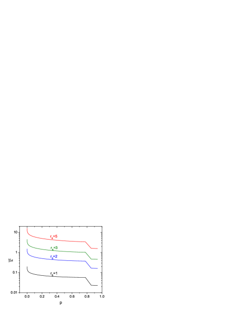
Figure 8: The behavior of $\gamma_{\bot}\tau$ as a function of polarization for various $r_{s}$. We assume $E_{F}\tau/\hbar=10/r_{s}^{2}$ and $k_{B}T/E_{F}=r_{s}^{2}/10$

For zero polarization the transverse spin-Coulomb drag coefficient coincides with the longitudinal one because of the isotropy of the electron gas. The behavior of the transverse spin-Coulomb drag coefficient is presented in Fig. 8 for various values of $r_{s}$. The effect of the electron-electron interactions is stronger for larger $r_{s}$ and therefore $\gamma_{\bot}\tau$ is larger. For a given $r_{s}$, $\gamma_{\bot}$ decreases with increasing polarization and saturates for large polarizations to the value of $\gamma\tau_{\bot}$ corresponding to the value of the $F(x,p)$ integral for $p=1$ (see Eq. (98)). The downward step at polarization $p=0.8$ is due to the fact that the limits of integration for $F(r_{s},-p)$ come together at this value of $p$ and furthermore the integrand has a singularity that causes the integral to drop to zero discontinuously at this point.

X Appendix D: Direct Matsubara calculation of the noninteracting transverse spin response

The Gilbert damping constant is directly related to the imaginary part of the transverse spin susceptibility, which does not depend on the equilibrium parameters (for example magnetization) of the system. It is useful to show that the calculation of the transverse spin susceptibility via the torque-torque correlator and the more direct calculation by Matsubara approach are equivalent. We consider the same Hamiltonian as in Eq. (38). The transverse spin response $\chi_{-+}$ is defined as follows:

$$\chi_{-+}(\mathbf{r},\mathbf{r^{\prime}};t,t^{\prime})=\frac{ig^{2}}{2V}\Theta(t-t^{\prime})\left\langle\left[s_{-}(\mathbf{r},t),s_{+}(\mathbf{r^{\prime}},t^{\prime})\right]\right\rangle\,,$$ (100)

where $\mathbf{s}(\mathbf{r})=\mbox{Tr}[\boldsymbol{\hat{\sigma}}\hat{\rho}(\mathbf{r})/4]$ is the spin density ($s_{\pm}=s_{x}\pm is_{y}$) in terms of the density matrix $\rho_{\alpha\beta}(\mathbf{r})=\Psi^{\dagger}_{\beta}(\mathbf{r})\Psi_{\alpha}(\mathbf{r})$.

It is straightforward to show that the disorder-averaged retarded single-particle Green’s function in the representation of Rashba subbands is given by

$$\hat{G}^{R}(\mathbf{k},\mathbf{k^{\prime}};\omega)=\delta_{\mathbf{k},\mathbf{k^{\prime}}}\hat{U}_{\mathbf{k}}\left(\begin{array}[]{cc}G_{+}^{R}(\mathbf{k},\omega)&0\\ 0&G_{-}^{R}(\mathbf{k},\omega)\end{array}\right)\hat{U}_{\mathbf{k}}\,,$$ (101)

where

$$G_{\pm}^{R}(\mathbf{k},\omega)=\frac{1}{\omega-(\epsilon_{k}\pm\\ \Omega)+i/2\tau}\,,$$ (102)

$\epsilon_{k}=\hbar^{2}k^{2}/2m-\mu$ , and $\hat{U}_{\mathbf{k}}$ are spin-rotation matrices:

$$\hat{U}_{\mathbf{k}}=\left(\begin{array}[]{cc}\cos(\delta/2)&i\sin(\delta/2)e^{-i\varphi_{\mathbf{k}}}\\ -i\sin(\delta/2)e^{i\varphi_{\mathbf{k}}}&-\cos(\delta/2)\end{array}\right)\,,$$ (103)

where

$$\cos\delta\equiv\frac{\omega_{0}}{\Omega}=\frac{p}{\sqrt{p^{2}+\bar{\alpha}^{2}}}~{},$$ (104)

and

$$\Omega\equiv\sqrt{\omega_{0}^{2}+\alpha^{2}k_{F}^{2}}$$ (105)

are defined as in main text. Note that, in general, $\hat{G}^{A}=(\hat{G}^{R})^{\dagger}$, in order to obtain the advanced Green’s function.

We do not assume any a priori hierarchy in the three energy scales $H$, $\alpha k_{F}$, and $1/\tau$, but we consider for simplicity the limit $\epsilon/\epsilon_{F}\ll 1$, where $\epsilon$ is any of the mentioned energy scales. Disregarding terms of order $\epsilon/\epsilon_{F}$, $k$ can be set to $k_{F}$ in the relevant expressions.

It is most convenient to calculate the spin response function in the Matsubara formalism. For a uniform perturbation, one gets in general

$$\chi_{-+}(i\bar{\Omega}_{n})=-\frac{g^{2}T}{2V^{2}}\sum_{\mathbf{k},\mathbf{k^{\prime}};m} G_{\uparrow\uparrow}(\mathbf{k^{\prime}},\mathbf{k};i\omega_{m})$$

$$\times G_{\downarrow\downarrow}(\mathbf{k},\mathbf{k^{\prime}};i\omega_{m}+i\bar{\Omega}_{n})\,,$$ (106)

where $\omega_{m}=2\pi T(m+1/2)$ and $\bar{\Omega}_{n}=2\pi Tn$ are fermionic and bosonic Matsubara frequencies, respectively. $T$ is the absolute temperature and $V$ the total volume of the system. The desired retarded response function is obtained by analytic continuation $i\bar{\Omega}_{n}\to\omega+i0^{+}$.

It is important to take into account vertex corrections when averaging Eq. (106) over disorder. Otherwise, the response would have a low-frequency dissipative component even in the absence of SO interaction, i.e., $\alpha=0$, if the disorder-averaged Green’s functions where inserted in Eq. (106). Namely, we find without vertex corrections:

$$\left.\partial_{\omega}\mbox{Im}\chi_{-+}(\omega)\right|_{\omega=0}=\frac{g^{2}}{V}\frac{m^{\ast}\tau}{8\pi}\left[\frac{1+\cos^{2}\delta}{1+(\Omega\tau)^{2}}+\sin^{2}\delta\right]\,,$$ (107)

which diverges in the clean limit, $\tau\to\infty$, even when there is no SO interaction, i.e., $\delta=0$, and vanishes in the dirty limit, $\tau\to 0$.

Taking into account vertex corrections is conceptually straightforward but technically somewhat tedious. Defining the tensor $\tensor{\Pi}$:

$$\Pi_{\alpha^{\prime}\beta,\alpha\beta^{\prime}}(i\bar{\Omega}_{n})=\sum_{\mathbf{k}\mathbf{k^{\prime}},m} G_{\alpha^{\prime}\beta}(\mathbf{k^{\prime}},\mathbf{k};i\omega_{m})$$

$$\times G_{\alpha\beta^{\prime}}(\mathbf{k},\mathbf{k^{\prime}};i\omega_{m}+i\bar{\Omega}_{n})\,,$$ (108)

whose $\uparrow\uparrow,\downarrow\downarrow$ component determines the response function according to Eq. (106), namely, $\chi_{-+}=-(T/2V)\Pi_{\uparrow\uparrow,\downarrow\downarrow}$,we find by summing the ladder diagrams

$$\Pi_{\alpha^{\prime}\beta,\alpha\beta^{\prime}}(i\bar{\Omega}_{n})=\sum_{m} \Gamma_{\alpha^{\prime}i,j\beta^{\prime}}(i\bar{\Omega}_{n},i\omega_{m})$$

$$\times\Upsilon_{i\beta,\alpha j}(i\bar{\Omega}_{n},i\omega_{m})\,,$$ (109)

where

$$\Upsilon_{\alpha^{\prime}\beta,\alpha\beta^{\prime}}(i\bar{\Omega}_{n},i\omega_{m})=\sum_{\mathbf{k}} G_{\alpha^{\prime}\beta}(\mathbf{k};i\omega_{m})$$

$$\times G_{\alpha\beta^{\prime}}(\mathbf{k};i\omega_{m}+i\bar{\Omega}_{n})\,,$$ (110)

is the $\omega_{m}$ contribution to the $\tensor{\Pi}$ tensor without the vertex corrections and

$$\Gamma_{\alpha^{\prime}\beta,\alpha\beta^{\prime}} (i\bar{\Omega}_{n},i\omega_{m})=\delta_{\alpha^{\prime}\beta}\delta_{\alpha\beta^{\prime}}+\frac{1}{2\pi\nu\tau}$$

$$\times\Gamma_{i\beta,\alpha j}(i\bar{\Omega}_{n},i\omega_{m})\Upsilon_{\alpha^{\prime}i,j\beta^{\prime}}(i\bar{\Omega}_{n},i\omega_{m})$$ (111)

is the recursive relation for the vertex tensor $\tensor{\Gamma}$. $\nu=m^{\ast}/2\pi$ is the density of states per spin. If a tensor $\tensor{A}$ can be decomposed into matrices $\hat{B}$ and $\hat{C}$ by $A_{\alpha^{\prime}\beta,\alpha\beta^{\prime}}=B_{\alpha^{\prime}\beta}C_{\alpha\beta^{\prime}}$, I will write $\tensor{A}=\hat{A}\otimes\hat{B}$. All subscripts in Eqs. (109), (110), and (111) are spin-$1/2$ indices taking values $\uparrow$ and $\downarrow$, and the summation over repeated indices $i$ and $j$ is implied.

In order to calculate the $\tensor{\Pi}$ tensor (109), we first follow the standard procedure of replacing the sum over $m$ by the integral $\int_{C}dz\tanh(z/2T)$ with the contour $C$ around the imaginary axis. The contour is then deformed towards the $\pm\infty$ along the real axis, around the branch cuts at $\mbox{Im}z=0$ and $i\bar{\Omega}_{n}$. Performing integrals over the branch cuts, we get

$$\tensor{\Pi}(\omega)=\int_{-\infty}^{\infty}\frac{d\epsilon}{4\pi iT\xi}\tanh\left(\frac{\epsilon}{2T}\right)\left[\tensor{\chi}^{R,R}(\epsilon,\epsilon+\omega)\right.$$

$$\left.-\tensor{\chi}^{A,R}(\epsilon,\epsilon+\omega)+\tensor{\chi}^{A,R}(\epsilon-\omega,\epsilon)-\tensor{\chi}^{A,A}(\epsilon-\omega,\epsilon)\right]\,,$$ (112)

where

$$\tensor{\chi}^{X,Y} (\epsilon,\epsilon^{\prime})=\tensor{\chi}^{X,Y}_{0}(\epsilon,\epsilon^{\prime})$$

$$+\xi\sum_{\mathbf{k}}\hat{G}^{X}(\mathbf{k},\epsilon)\tensor{\chi}^{X,Y}(\epsilon,\epsilon^{\prime})\hat{G}^{Y}(\mathbf{k},\epsilon^{\prime})$$ (113)

is the recursion relation corresponding to Eq. (111) ($X,Y=A~{}{\rm or}~{}R$ and $\xi^{-1}=2\pi\nu\tau V$) and

$$\tensor{\chi}^{X,Y}_{0}(\epsilon,\epsilon^{\prime})=\xi\sum_{\mathbf{k}}\hat{G}^{X}(\mathbf{k},\epsilon)\otimes\hat{G}^{Y}(\mathbf{k},\epsilon^{\prime})\,.$$ (114)

Since we are interested in dissipation, let us define $2\mbox{Im}\tensor{\Pi}=-i(\tensor{\Pi}-\tensor{\Pi}^{\dagger})$, where $\{{\tensor{\Pi}^{\dagger}}\}_{\alpha^{\prime}\beta,\alpha\beta^{\prime}}=\Pi_{\beta\alpha^{\prime},\beta^{\prime}\alpha}^{\ast}$. We then take the following steps in order to evaluate $\mbox{Im}\tensor{\Pi}$: First, Eq. (113) is iteratively expanded in terms of the disorder-averaged Green’s functions $\hat{G}^{X}$, then the “unrolled” $\tensor{\chi}^{X,Y}$ is substituted into Eq. (112). Differentiating the resulting expression with respect to $\omega$ and taking the imaginary part, the integral can be transformed integrating by parts into $\int d\epsilon\tanh(\epsilon/2T)\partial_{\epsilon}...=-\int d\epsilon\partial_{\epsilon}\tanh(\epsilon/2T)...$, and, assuming low temperatures, we approximate $\partial_{\epsilon}\tanh(\epsilon/2T)\approx 2\delta(\epsilon)$, so that the dissipation is naturally governed by electron-hole pair excitations near the Fermi surface. The infinite summation series is finally “rolled” back into a recursive relation and we obtain the following expression for the spin response:

$$\left.\partial_{\omega}\mbox{Im}\chi_{-+}(\omega)\right|_{\omega=0}= -\frac{g^{2}}{V}\frac{m^{\ast}\tau}{8\pi}$$

$$\times\left(\tensor{\chi}^{R,R}-\tensor{\chi}^{A,R}-\tensor{\chi}^{R,A}+\tensor{\chi}^{A,A}\right)_{\uparrow\uparrow,\downarrow\downarrow}\,,$$ (115)

where all $\tensor{\chi}$’s are now evaluated at $\epsilon,\epsilon^{\prime}=0$.

The problem is thus reduced to calculating $\tensor{\chi}^{X,Y}(0,0)$ using Eqs. (113) and (114). It is still somewhat tedious but now totally straightforward. We first do the angular integration fixing the absolute value of $\mathbf{k}$ in Eq. (114). This averages over the rotation matrices (103). The resulting angle-averaged tensor (114) then decomposes into 6 components: $\hat{1}\otimes\hat{1}$, $\hat{1}\otimes\hat{\sigma}_{z}$, $\hat{\sigma}_{z}\otimes\hat{1}$, $\hat{\sigma}_{z}\otimes\hat{\sigma}_{z}$, $\hat{\sigma}_{+}\otimes\hat{\sigma}_{-}$, and $\hat{\sigma}_{-}\otimes\hat{\sigma}_{+}$ (the last two are solely due to the SO coupling), where $\hat{\sigma}_{\pm}=\hat{\sigma}_{x}\pm i\hat{\sigma}_{y}$. The respective prefactors are given by integrals over the absolute value of momentum near the Fermi energy, which are trivial to evaluate after linearizing the dispersion at the Fermi level. We then make an ansatz that the tensor $\tensor{\chi}^{X,Y}(0,0)$ determined by Eq. (113) can also be expanded in terms of the same 6 components and, after plugging the expanded $\tensor{\chi}^{X,Y}$ (with unknown coefficients) and $\tensor{\chi}^{X,Y}_{0}$ (with calculated coefficients) into Eq. (113), we obtain a linear system of equations for the unknown coefficients that determine $\tensor{\chi}^{X,Y}$. Solving this (with Mathematica), we find a solution (validating the ansatz), and the dissipative part of the spin response is finally given by

$$\left.\partial_{\omega}\mbox{Im}\chi_{-+}(\omega)\right|_{\omega=0}= \frac{g^{2}}{V}\frac{m^{\ast}\tau}{8\pi}\sin^{2}\delta$$

$$\times\frac{1+\frac{1}{2}(\Omega\tau)^{2}(1+\cos^{2}\delta)}{\cos^{2}\delta+\frac{1}{4}(\Omega\tau)^{2}(1+\cos^{2}\delta)^{2}}\,,$$ (116)

Using Eq. (26) and Eq. (30) one can show that Gilbert damping has a following form:

$$\lambda=gM_{0}V\lim_{\omega\rightarrow 0}\frac{\partial_{\omega}\mbox{Im}\chi_{-+}(\omega)}{\chi^{2}_{0}(\omega=0)}=$$

$$p\frac{E_{F}\tau\sin^{2}\delta}{\hbar}\frac{1+\frac{1}{2}(\Omega\tau)^{2}(1+\cos^{2}\delta)}{\cos^{2}\delta+\frac{1}{4}(\Omega\tau)^{2}(1+\cos^{2}\delta)^{2}}~{}$$ (117)

in agreement with Eq. (55).

References

• Gilbert (1955) T. L. Gilbert, Phys. Rev. 100, 1243 (1955).
• Gilbert (2004) T. L. Gilbert, IEEE Trans. Magn. 40, 3443 (2004).
• Lifshitz and Pitaevskii (1980) E. M. Lifshitz and L. P. Pitaevskii, Statistical Physics, Part 2, vol. 9 of Course of Theoretical Physics (Pergamon, Oxford, 1980), 3rd ed.
• Tserkovnyak et al. (2005) Y. Tserkovnyak, A. Brataas, G. E. Bauer, and B. I. Halperin, Rev. Mod. Phys. 77, 1375 (2005).
• Tserkovnyak et al. (2002a) Y. Tserkovnyak, A. Brataas, and G. E. W. Bauer, Phys. Rev. Lett. 88, 117601 (2002a).
• Tserkovnyak et al. (2002b) Y. Tserkovnyak, A. Brataas, and G. E. W. Bauer, Phys. Rev. B 66, 224403 (2002b).
• Heinrich et al. (1967) B. Heinrich, D. Fraitová, and V. Kamberský, Phys. Status Solidi 23, 501 (1967).
• Korenman and Prange (1972) V. Korenman and R. E. Prange, Phys. Rev. B 6, 2769 (1972).
• Lutovinov and Reizer (1979) V. S. Lutovinov and M. U. Reizer, Sov. Phys. JETP 50, 355 (1979).
• Solontsov and Vasil’ev (1993) A. Z. Solontsov and A. N. Vasil’ev, Phys. Lett. A 177, 362 (1993).
• Suhl (1998) H. Suhl, IEEE Trans. Magn. 34, 1834 (1998).
• Heinrich et al. (2002) B. Heinrich, R. Urban, and G. Woltersdorf, IEEE Trans. Magn. 38, 2496 (2002).
• Kuneš and Kamberský (2002) J. Kuneš and V. Kamberský, Phys. Rev. B 65, 212411 (2002).
• Dobin and Victora (2003) A. Y. Dobin and R. H. Victora, Phys. Rev. Lett. 90, 167203 (2003).
• Sinova et al. (2004a) J. Sinova, T. Jungwirth, X. Liu, Y. Sasaki, J. K. Furdyna, W. A. Atkinson, and A. H. MacDonald, Phys. Rev. B 69, 085209 (2004a).
• Tserkovnyak et al. (2004) Y. Tserkovnyak, G. A. Fiete, and B. I. Halperin, Apl. Phys. Lett. 84, 5234 (2004).
• Koopmans et al. (2005) B. Koopmans, J. J. M. Ruigrok, F. Dalla Longa, and W. J. M. de Jonge, Phys. Rev. Lett. 95, 267207 (2005).
• Steiauf and Fähnle (2005) D. Steiauf and M. Fähnle, Phys. Rev. B 72, 064450 (2005).
• (19) Y. Tserkovnyak, H. J. Skadsem, A. Brataas, and G. E. W. Bauer, cond-mat/0512715.
• (20) H. Kohno, G. Tatara, and J. Shibata, cond-mat/0605186.
• Mizukami et al. (2002) S. Mizukami, Y. Ando, and T. Miyazaki, Phys. Rev. B 66, 104413 (2002).
• Ingvarsson et al. (2002) S. Ingvarsson, L. Ritchie, X. Y. Liu, G. Xiao, J. C. Slonczewski, P. L. Trouilloud, and R. H. Koch, Phys. Rev. B 66, 214416 (2002).
• Burkov and Balents (2004) A. A. Burkov and L. Balents, Phys. Rev. B 69, 245312 (2004).
• Murakami et al. (2003) S. Murakami, N. Nagaosa, and S.-C. Zhang, Science 301, 1348 (2003).
• Sinova et al. (2004b) J. Sinova, D. Culcer, Q. Niu, N. A. Sinitsyn, T. Jungwirth, and A. H. MacDonald, Phys. Rev. Lett. 92, 126603 (2004b).
• Kato et al. (2004) Y. K. Kato, R. C. Myers, A. C. Gossard, and D. D. Awschalom, Science 306, 1910 (2004).
• Wunderlich et al. (2005) J. Wunderlich, B. Kaestner, J. Sinova, and T. Jungwirth, Phys. Rev. Lett. 94, 047204 (2005).
• Sih et al. (2006) V. Sih, W. H. Lau, R. C. Myers, V. R. Horowitz, A. C. Gossard, and D. D. Awschalom, Phys. Rev. Lett. 97, 096605 (2006).
• Konig et al. (2006) M. Konig, A. Tschetschetkin, E. M. Hankiewicz, J. Sinova, V. Hock, V. Daumer, M. Schafer, C. R. Becker, H. Buhmann, and L. W. Molenkamp, Phys. Rev. Lett. 96, 076804 (2006).
• D’Amico and Vignale (2000) I. D’Amico and G. Vignale, Phys. Rev. B 62, 4853 (2000).
• D’Amico and Vignale (2002) I. D’Amico and G. Vignale, Phys. Rev. B 65, 85109 (2002).
• Qian and Vignale (2002) Z. Qian and G. Vignale, Phys. Rev. Lett. 88, 056404 (2002).
• Mishchenko et al. (2004) E. G. Mishchenko, A. V. Shytov, and B. I. Halperin, Phys. Rev. Lett. 93, 226602 (2004).
• (34) S. P. P. S. Ingvarsson, G. Xiao and R. H. Koch, eprint cond-mat/0408608.