Statistical-mechanical theory of ultrasonic absorption in molecular liquids

Abstract

We present results of theoretical description of ultrasonic phenomena in molecular liquids. In particular, we are interested in the development of microscopical, i.e., statistical-mechanical framework capable to explain the long living puzzle of the excess ultrasonic absorption in liquids. Typically, ultrasonic wave in a liquid can be generated by applying the periodically alternating external pressure with the angular frequency that corresponds to the ultrasound. If the perturbation introduced by such process is weak – its statistical-mechanical treatment can be done with the use of the linear response theory. We treat the liquid as a system of interacting sites, so that all the response/aftereffect functions as well as the energy dissipation and generalized (wave-vector and frequency dependent) ultrasonic absorption coefficient are obtained in terms of familiar site-site static and time correlation functions such as static structure factors or intermediate scattering functions. To express the site-site intermediate scattering functions we refer to the site-site memory equations in the mode-coupling approximation for the first-order memory kernels, while equilibrium properties such as site-site static structure factors, direct and total correlation functions are deduced from the integral equation theory of molecular liquids known as RISM or one of its generalizations. All the formalism is phrased in a general manner, hence the obtained results are expected to work for arbitrary type of molecular liquid including simple, ionic, polar, and non-polar liquids.

I Introduction

Sound velocity and absorption are important probes of physical and chemical processes taking place in liquid and liquid mixtures Herzfeld59 ; Bhatia67 . Sound velocity reflects density fluctuations occurring in solutions, thereby, it is closely related to the compressibility, which is a response function of the density to the mechanical perturbation, or pressure. The property is probably the best measure for the mechanical stability of solutions. On the other hand, sound absorption probes the energy dissipation caused by a variety of irreversible processes taking place in solutions: for example, structural relaxation of liquids, conformational transition of molecules in solution, and so forth. No wonder why people have employed the method for long time to investigate the structure and dynamics in solutions. There has been enormous amount of experimental data accumulated in the filed of science and technology. More importantly, the method seems to be finding new horizon in different fields of scientific research Shutilov88 ; Povey97 ; Cheeke02 ; Dukhin02 ; Kundu04 , not mentioning about the usage in medicine and pharmacy Hill04 ; Rumack05 ; Attwood81 ; Tolley83 ; Tata93 ; Ishihara93 ; Jeffers95 ; Tachibana98 ; Curra03 ; Wu05 . Especially important among the applications is that to the stability and conformational transition of biomolecules such as protein. The sound velocity and the adiabatic compressibility have already been on duty to clarifying the mechanical stability of protein in solution Gavish83 ; Gekko79 ; Gekko89 ; Gekko91 . At the frontier in the science, sound velocity has been employed to identify the conformational transition from native to denatured states of protein (for the effect of ultrasound on biological molecules and macromolecules see, e.g., Refs. Choi86 ; Choi87 ; Bae96 ; Sakai00 ; Pethrick83 ; Pavlovskaya92 ; Kharakoz89 ; Kharakoz91 ; Kharakoz93 ; Ravichandran91 ; Shin94 ; Chalikian95 ; Kitamura95 ; Karabutov98 ). It won’t be so long before the sound absorption associated with the conformational relaxation is determined by the acoustic measurement. The method seems appropriate to investigate the large scale fluctuation or the collective dynamics characteristic to the macromolecule, because the frequency range of such motion is covered by that of sound wave. However, there exists a high barrier for the method to be overcome in order to be applied to the field. That is the method or theory to analyze the experimental observations.

Traditional ways of interpreting data from acoustic measurements are based on the hydrodynamic and/or the phenomenological theories of relaxation Landau84 ; Richards39 ; Markham51 ; Bauer49 ; Gierer50a ; Teubner79 ; Bhattacharjee81 ; Narasimham90 ; Martynov01 ; Delgado05 exemplified by that of Debye-type and of stretched-exponential-type. Those theories inevitably require phenomenological and/or molecular models for the relaxation, which sometimes are far from reality. One of the most successful theories of the sound absorption is that for water, proposed by Hall more than half a century ago Hall47 ; Hall48 . Hall has assumed that water is an equilibrium mixture of two states: monomers having densely packed structure and hydrogen-bonded clusters which have an ice-like open-packed structure. The equilibrium will shift toward the monomers by acoustic pressure due to the difference in the molar volume between the two components of the mixture. The energy dissipation associated with the relaxation process is probed by the sound absorption. Hall applied the transition state theory to the two-state model in order to explain the sound absorption by liquid water. The treatment should be remarked as the most important contemporary achievement in theories of sound absorption by liquids, because it is the first theory to relate the acoustic process with the microscopic model of the liquid structure.

Unfortunately, the progress seems stopped at the level of Hall as far as the microscopic treatment of the sound absorption is concerned with. The reason is simply because Hall’s theory employs a structural model for the liquid. It means that the theory requires a model for liquid structure for each liquid or solution, and phenomenological or empirical parameters associated with the model, such as the molar volume. The difficulty of constructing a model for liquid structure will be easily understood by taking the water-alcohol mixture as an example. All those are suggesting that the theory of sound absorption is necessary to start from a Hamiltonian level or a molecular interaction, not from structural models of liquid.

One may think it will then be appropriate to employ the molecular dynamics simulation, because the method starts definitely from the Hamiltonian model. However, the problem is formidably difficult for the method, because it touches both the hydrodynamic and thermodynamic limits. Just imagine the typical wave length of the ultrasonic wave, and how many molecules should be involved in a wave packet. But if the simulation is technically feasible, it does not help much, because the analysis of trajectory will require the statistical mechanics of molecular liquids. Without having a method of analysis, the trajectory is just a garbage.

The present paper aims to construct a molecular theory of sound absorption based on the latest development in the statistical mechanics, or the site-site representation of the generalized Langevin theory. The theory combines two elements in the theoretical physics: the reference interaction site model (RISM) and the generalized Langevin equation (GLE). The RISM theory is an integral equation method to describe equilibrium structure of molecular liquids in terms of the site-site pair correlation functions, from which all the thermodynamic quantities can be derived Hirata81 ; Hirata82 ; Hirata83 ; Hirata03 . The theory and its three dimensional generalization have been applied successfully to almost entire spectrum of chemical and physical processes taking place in solution from chemical reactions to the molecular recognition by protein Hirata03 ; Imai05 ; Yoshida06 . Among the applications, the results for the isothermal compressibility of the water-butanol mixture Omelyan03 are of particular interest in conjunction with the present topics, since it is closely related to the mechanical stability of solutions. The theory could have successfully reproduced the concentration and temperature dependence of the compressibility of the solution observed experimentally, and it could have been able to describe the behavior in terms of the liquid structure. In that sense, the theory has already demonstrated its capability to explain the molecular mechanism of sound velocity. However, it is not complete for describing the entire physics of sound propagation, because it is in general accompanied by energy dissipation, or attenuation of sound wave. This is the reason why we employ the GLE theory – a statistical mechanics theory for irreversible processes. In past two decades, we have developed a method which combines RISM and GLE Hirata03 . The method could have described a variety of irreversible processes with great success, including the ion transport Chong98 , dynamics of water Chong99a ; Chong99b , viscosity Yamaguchi01 , dielectric relaxation Yamaguchi03a , translational and rotational dynamics of a molecule in solutions Yamaguchi04b ; Kobryn05 ; Kobryn06 . Especially important in relation with the present topic is the contribution made by Yamaguchi et al. Yamaguchi03b who formulated a theory for ultrasonic vibration potential, or the coupling of acoustic and electrostatic perturbations in polar liquids. This work provides a good guide for the development of a theory of ultrasonic phenomena in liquids.

In the present paper, we propose a theory for sound absorption in molecular liquids based on combination of the RISM theory, the GLE theory, and the linear response theory. Starting from definition of the perturbation Hamiltonian which describes the coupling of the sound wave and a liquid system, we derive an expression for the sound absorption in the most general form. In the choice of parameters for abbreviated description we recognize that the traditionally employed set of fluctuations of local site densities and longitudinal site currents is not enough to serve our purposes in this case and has to be extended by adding fluctuations of the total energy density. The latter is really necessary if one wants to obtain in the expression for ultrasonic absorption coefficient terms related to the thermal conductivity of the system. We then apply the theory to the simplest case of a liquid of spherical molecules and derive expressions in the hydrodynamic limit in order to make contact with the result from classical hydrodynamics.

The paper is organized as follows. In Section II we specify the system, define basic dynamical quantities that we use for its description, and write their equations of motion. In Section III we provide derivation of the perturbation Hamiltonian for the case of not too strong ultrasonic vibrations so that the result of derivation can be used in the theory of linear response. Application of the theory of linear response to our system is described in Section IV, where we calculate linear responses of local particle number, charge and mass densities for the perturbation caused by the propagating ultrasonic wave. All responses are written in terms of familiar static and time correlation functions. A major step to calculate ultrasonic absorption coefficient is made in Section V, where we first derive an expression for the energy dissipation, and then use it to define the generalized, i.e., wave-vector and frequency dependent ultrasonic absorption coefficient in a liquid. For that purpose one may require the knowledge of site-site intermediate scattering functions. Therefore another and rather big portion of the material is dedicated to the problem of their calculation and is put in Sections VI and VII. The remaining part of the paper is about detailed analysis of our findings. In particular, we consider the hydrodynamic limit of our result for the case of one-component simple liquid in order to compare it with the one from the continuous media models Herzfeld59 ; Bhatia67 ; Landau84 . The required steps and their consequences are described in Section VIII. Finally, advances, deficiencies, remedies and open questions of our treatment are summarized in Section IX. Auxiliary material is put into Appendices.

II Definition of the system and variables

Let us give first generic definitions of major quantities for a mixture of $\mathcal{M}$-component classical molecular liquid confined in volume $V$. We suppose that each component consists of $N_{\mu}$ particles (and indices $\mu,\nu=1,\ldots,\mathcal{M}$ are used to label molecular species), hence the total number of particles is $\sum_{\mu}N_{\mu}=N$. According to this, $x_{\mu}=N_{\mu}/N$ should be particle relative concentrations (or molar fractions). Each molecule consists of $\Lambda_{\mu}$ sites (could be atoms) having charges $z_{\mu}^{\alpha}$ and masses $m_{\mu}^{\alpha}$ (and indices $\alpha,\gamma=1,\ldots,\Lambda_{\mu}$ are used to label molecular sites). Time-dependent positions and momenta of individual sites will be denoted then as $\mathbf{r}_{\mu,i}^{\alpha}(t)$ and $\mathbf{p}_{\mu,i}^{\alpha}(t)=m_{\mu}^{\alpha}\mathbf{v}_{\mu,i}^{\alpha}(t)$, respectively, with $\mathbf{v}_{\mu,i}^{\alpha}(t)$ being site velocities.

Let us suppose that the unperturbed system in concern is described by the Hamiltonian $H$, and that the perturbation introduced by the external pressure $P$ is $H^{\prime}$. Microscopic expression for $H$ can be written as the sum of the kinetic $H_{\text{kin}}$ and interaction $H_{\text{int}}$ parts as

$$H = H_{\text{kin}}+H_{\text{int}},$$ (1a)

$$H_{\text{kin}} = \sum_{\mu=1}^{\mathcal{M}}\sum_{i=1}^{N_{\mu}}\sum_{\alpha=1}^{\Lambda_{\mu}}\frac{\left[p_{\mu,i}^{\alpha}(t)\right]^{2}}{2m_{\mu}^{\alpha}},$$ (1b)

$$H_{\text{int}} = \sum_{\mu=1}^{\mathcal{M}}\sum_{i=1}^{N_{\mu}}\sum_{\alpha=1}^{\Lambda_{\mu}}\sum_{\nu=1}^{\mathcal{M}}\sum_{j=1}^{N_{\nu}}\sum_{\gamma=1}^{\Lambda_{\nu}}\phi_{\mu\nu,ij}^{\alpha\gamma}\left(|\mathbf{r}_{\mu\nu,ij}^{\alpha\gamma}(t)|\right),\qquad$$ (1c)

where $\mathbf{r}_{\mu\nu,ij}^{\alpha\gamma}(t)\equiv\mathbf{r}_{\mu,i}^{\alpha}(t)-\mathbf{r}_{\nu,j}^{\gamma}(t)$, and $\phi_{\mu\nu,ij}^{\alpha\gamma}(|\mathbf{r}_{\mu\nu,ij}^{\alpha\gamma}(t)|)$ is potential of interaction between sites, also it is assumed implicitly that if $\nu=\mu$, then $j\not=i$ (in the following, this condition will be indicated by the prime mark next to the summation symbol). At present, a detailed knowledge of structure for $\phi_{\mu\nu,ij}^{\alpha\gamma}(|\mathbf{r}_{\mu\nu,ij}^{\alpha\gamma}(t)|)$ is not required. For simplicity of notations we will denote the triplicate sum by a symbol as follows

$$\sum_{\mu=1}^{\mathcal{M}}\sum_{i=1}^{N_{\mu}}\sum_{\alpha=1}^{\Lambda_{\mu}}\longrightarrow\sum_{\text{\char 172}},\quad\sum_{\nu=1}^{\mathcal{M}}\sum_{j=1}^{N_{\nu}}\sum_{\gamma=1}^{\Lambda_{\nu}}\longrightarrow\sum_{\text{\char 173}}.$$ (2)

Equations of motion for individual site positions and momenta are the Hamilton equations

$$\dot{\mathbf{r}}_{\mu,i}^{\alpha}(t) = \frac{\partial H}{\partial\mathbf{p}_{\mu,i}^{\alpha}(t)},$$ (3a)

$$\dot{\mathbf{p}}_{\mu,i}^{\alpha}(t) = -\frac{\partial H}{\partial\mathbf{r}_{\mu,i}^{\alpha}(t)}.$$ (3b)

They are used to derive microscopic equations of motion for dynamical variables. Microscopic single-particle density and momentum density are defined, respectively, as

$$\rho_{\mu,i}^{\alpha}(\mathbf{r};t) = \delta\left(\mathbf{r}-\mathbf{r}_{\mu,i}^{\alpha}(t)\right),$$ (4a)

$$\mathbf{p}_{\mu,i}^{\alpha}(\mathbf{r};t) = \mathbf{p}_{\mu,i}^{\alpha}(t)\delta\left(\mathbf{r}-\mathbf{r}_{\mu,i}^{\alpha}(t)\right),$$ (4b)

with $\delta(\mathbf{r})$ being the 3d Dirac $\delta$-function. Next we introduce collective variables such as particle number-density $\rho(\mathbf{r};t)$, particle charge-density $\rho_{\text{{c}}}(\mathbf{r};t)$ and particle mass-density $\rho_{\text{{m}}}(\mathbf{r};t)$, for which we will use common designation $\bbrho(\mathbf{r};t)$, so that

$$\bbrho(\mathbf{r};t) = \Big{\{}\rho(\mathbf{r};t),\rho_{\text{{c}}}(\mathbf{r};t),\rho_{\text{{m}}}(\mathbf{r};t)\Big{\}}$$ (5)

$$= \sum_{\text{\char 172}}\rho_{\mu,i}^{\alpha}(\mathbf{r};t)\left\{1,z_{\mu}^{\alpha},m_{\mu}^{\alpha}\right\},$$

$$= \sum_{\text{\char 172}}\rho_{\mu,i}^{\alpha}(\mathbf{r};t)\Upsilon_{\mu}^{\alpha},$$

where $\Upsilon_{\mu}^{\alpha}$ is used to denote the set $\{1,z_{\mu}^{\alpha},m_{\mu}^{\alpha}\}$. For the system in equilibrium $\langle\rho(\mathbf{r};t)\rangle=\rho$, $\langle\rho_{\text{{c}}}(\mathbf{r};t)\rangle=0$ and $\langle\rho_{\text{{m}}}(\mathbf{r};t)\rangle=\rho_{\text{{m}}}$, where $\rho$ is the mean value of the particle number-density and $\rho_{\text{{m}}}$ is unperturbed mass-density. Angular brackets $\langle\ldots\rangle$ denote an appropriate statistical average: for example, the Gibbs canonical ensemble average.

Similarly, the particle number-density current $\mathbf{j}(\mathbf{r};t)$, charge-density current $\mathbf{j}_{\text{\sc c}}(\mathbf{r};t)$, and mass-density current $\mathbf{j}_{\text{\sc m}}(\mathbf{r};t)$, for which we also will use one common designation $\mathbb{j}(\mathbf{r};t)$, are defined as

$$\mathbb{j}(\mathbf{r};t) = \Big{\{}\mathbf{j}(\mathbf{r};t),\mathbf{j}_{\text{\sc c}}(\mathbf{r};t),\mathbf{j}_{\text{\sc m}}(\mathbf{r};t)\Big{\}}$$ (6)

$$= \sum_{\text{\char 172}}\mathbf{p}_{\mu,i}^{\alpha}(\mathbf{r};t)\frac{1}{m_{\mu}^{\alpha}}\Upsilon_{\mu}^{\alpha}.$$

It is worth to note, that $\mathbf{j}_{\text{\sc m}}(\mathbf{r};t)$ is nothing but the momentum-density, i.e., $\mathbf{j}_{\text{\sc{m}}}(\mathbf{r};t)\equiv\mathbf{p}(\mathbf{r};t)$. Its spacial integral is the total momentum of the system $\mathbf{P}$, which is the conserved quantity. By a suitable choice of the reference frame it can always be maid to vanish. In the following, we will assume that for the case of unperturbed system that condition is satisfied.

Energy density $\rho_{\text{{h}}}(\mathbf{r};t)$ can be introduced in a similar way, i.e., that its spatial integral is the total system energy, or the Hamiltonian $H$, and is therefore the conserved quantity. It is convenient to distinguish explicitly contributions from kinetic and interaction parts, so that the microscopic expression for $\rho_{\text{{h}}}(\mathbf{r};t)$ reads Zubarev74

$$\rho_{\text{{h}}}(\mathbf{r};t) = \rho_{\text{{\sc h},kin}}(\mathbf{r};t)+\rho_{\text{{\sc h},int}}(\mathbf{r};t),$$ (7a)

$$\rho_{\text{{\sc h},kin}}(\mathbf{r};t) = \sum_{\text{\char 172}}\frac{\left[p_{\mu,i}^{\alpha}(t)\right]^{2}}{2m_{\mu}^{\alpha}}\rho_{\mu,i}^{\alpha}(\mathbf{r};t),$$ (7b)

$$\rho_{\text{{\sc h},int}}(\mathbf{r};t) = \frac{1}{2}\int\textrm{d}\mathbf{r}^{\prime}\;\sideset{}{{}^{\prime}}{\mathop{\sum_{\text{\char 172,\char 173}}}}\phi_{\mu\nu,ij}^{\alpha\gamma}(|\mathbf{r}-\mathbf{r}^{\prime}|)f_{\mu\nu,ij}^{\alpha\gamma}(\mathbf{r},\mathbf{r}^{\prime};t),$$

where $f_{\mu\nu,ij}^{\alpha\gamma}(\mathbf{r},\mathbf{r}^{\prime};t)$ is a two-particle distribution function. Its general expression depends on many factors of the system and can be obtained, in principle, from the kinetic theory. In our consideration, however, we will use the approximation

$$\rho_{\text{{\sc h},int}}(\mathbf{r};t) \approx \frac{1}{2}\int\textrm{d}\mathbf{r}^{\prime}\sideset{}{{}^{\prime}}{\mathop{\sum_{\text{\char 172,\char 173}}}}\phi_{\mu\nu,ij}^{\alpha\gamma}(|\mathbf{r}-\mathbf{r}^{\prime}|)\makebox[7.00002pt][c]{\text{g}}_{\mu\nu,ij}^{\alpha\gamma}(|\mathbf{r}-\mathbf{r}^{\prime}|)$$ (8)

$${}\times\delta\left(\mathbf{r}-\mathbf{r}_{\mu,i}^{\alpha}(t)\right)\delta\left(\mathbf{r}^{\prime}-\mathbf{r}_{\nu,j}^{\gamma}(t)\right),$$

where $\makebox[7.00002pt][c]{\text{g}}_{\mu\nu,ij}^{\alpha\gamma}(|\mathbf{r}-\mathbf{r}^{\prime}|)$ is the radial distribution function that depends only on the mutual distance between sites.

Equations of motion for dynamical variables $\bbrho(\mathbf{r};t)$, $\mathbb{j}(\mathbf{r};t)$ and $\rho_{\text{\sc h}}(\mathbf{r};t)$ can be obtained with the use of Hamilton equations (3). In the reciprocal space they take the form of algebraic equations, since $\mathbf{k}$-dependent quantities $\bbrho(\mathbf{k};t)$, $\mathbb{j}(\mathbf{k};t)$ and $\rho_{\text{\sc h}}(\mathbf{k};t)$ are spatial 3d-Fourier transforms of their counterparts in the direct space (we use the same notations in both direct and reciprocal spaces and hope there will be no confusion since we distinguish functions by their arguments). In particular, equations of motion for quantities in concern read

$$\dot{\rho}_{\text{{m}}}(\mathbf{k};t) = i\mathbf{k}\cdot\mathbf{p}(\mathbf{k};t),$$ (9a)

$$\dot{\mathbf{p}}(\mathbf{k};t) = i\mathbf{k}:\mathbf{\Pi}(\mathbf{k};t),$$ (9b)

$$\dot{\rho}_{\text{{h}}}(\mathbf{k};t) = i\mathbf{k}\cdot\mathbf{j}_{\text{\sc h}}(\mathbf{k};t)+ih(\mathbf{k};t),$$ (9c)

where $\mathbf{\Pi}(\mathbf{k};t)$ is the Fourier transform of the stress tensor, and $\mathbf{j}_{\text{\sc h}}(\mathbf{k};t)$ and $h(\mathbf{k};t)$ are related with the Fourier transform of the energy current (its kinetic and interaction parts, respectively). For the moment, a detailed knowledge of their structure is not needed.

III The Perturbation Hamiltonian

In this section we are concerned about derivation of the perturbation Hamiltonian. Hence, it is worth to begin from considering the generation of ultrasonic waves and their propagation in a media. A typical type of the ultrasound source in action is displayed in Fig. 1. The sound field in front of a source is represented by means of lines of a constant phase, where the phase of a wave refers to the position of maximum or minimum in a wave. Experimental observations tell Herzfeld59 ; Bhatia67 that ultrasonic waves lose their intensity with penetration depth rapidly. It means that sonic amplitude in area called the far field is negligible. By considering a situation when the piston source oscillations produce the ultrasonic wave of relatively small amplitude, one may expect that the theory of linear response Kubo57a ; Kubo57b can be applied to describe the introduced perturbation almost everywhere in front of a piston starting from the near field and spreading forward to the area beyond the focus.

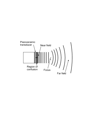
Figure 1: Piston source operating with the diameter (aperture) very much greater than the acoustic wavelength in the medium in contact with the front of the transducer Povey97 . The sound field in front of a piston source is drawn as lines of a constant phase, i.e., the positions of maximum or a minimum in a wave.

When the external pressure is applied to the system, the perturbed part $H^{\prime}$ of the total Hamiltonian $H_{\text{tot}}$ can be related to the work on changing of the deformation tensor $u_{\beta\delta}$ (here indices $\beta$, $\delta$ are used to denote Cartesian coordinates $x$, $y$, $z$). In the linear approximation this tensor is defined as Shutilov88

$$u_{\beta\delta}=\frac{1}{2}\left(\frac{\partial l_{\beta}}{\partial r_{\delta}}+\frac{\partial l_{\delta}}{\partial r_{\beta}}\right),$$ (10)

where $\mathbf{l}$ is the time-dependent displacement due to the periodically applied external pressure (which for definiteness we will think is applied along the $z$-axis of the system), and therefore should be presented as

$$\mathbf{l}\to\mathbf{l}(t)=\mathbf{a}\exp\left\{-i\left(\omega t+\varphi\right)\right\}$$ (11)

with $a=|\mathbf{a}|$, $\omega$ and $\varphi$ being the amplitude, angular frequency, and initial phase, respectively. Assuming that the displacement $\mathbf{l}(t)$ is sufficiently small (in the macroscopic scale), elementary work on changing the deformation tensor can be calculated as the internal stress force times the displacement. Total work is then obtained by integration over the volume of the system:

$$\int\textrm{d}V\;W(\mathbf{r};t)=\int\textrm{d}V\sum_{\beta,\delta}\frac{\partial\left[\boldsymbol{\Pi}(\mathbf{r};t)\right]_{\beta\delta}}{\partial\left[\mathbf{r}\right]_{\delta}}\left[\mathbf{l}(t)\right]_{\beta},$$ (12)

where $W(\mathbf{r};t)$ denotes the work of internal stress forces in unit volume. The density of this work is the density of the energy of elastic deformation and can be regarded as the density of the perturbation Hamiltonian $H^{\prime}(\mathbf{r};t)$. For the following consideration it is convenient to rewrite it as

$$H^{\prime}(\mathbf{r};t)=-M(\mathbf{r};t)E(t),$$ (13a)

where

$$M(\mathbf{r};t) = -\sum_{\beta,\delta}\frac{\partial\left[\boldsymbol{\Pi}(\mathbf{r};t)\right]_{\beta\delta}}{\partial\left[\mathbf{r}\right]_{\delta}}\left[\mathbf{a}\right]_{\beta}$$ (13b)

$$E(t) = \exp\left\{-i\left(\omega t+\varphi\right)\right\}.$$ (13c)

The reason for that will be seen later.

IV Linear responseto the acoustic perturbation

In the theory of linear response Kubo57a ; Kubo57b the total system Hamiltonian $H_{\text{tot}}$ is considered to be a sum of its regular part, say $H$, and perturbation, say $H^{\prime}$. If the density of the perturbed part can be written as $H^{\prime}(\mathbf{r};t)=-M(\mathbf{r};t)E(t)$, then in terms of the spatial Fourier components the time-dependent average linear response of a dynamical quantity $A(t)$ produced by the applied field $E(t)$ is given by

$$\langle A(\mathbf{k};t)\rangle_{\text{\o}}=-\frac{1}{k_{\mathrm{B}}T}\int_{-\infty}^{t}\textrm{d}s\langle\dot{A}(\mathbf{k};t-s)M(-\mathbf{k};0)\rangle E(s),$$ (14)

where $k_{\mathrm{B}}$ is the Boltzmann constant, $T$ is thermodynamic temperature, and the subscript ø is used to indicate the average of a perturbed quantity. An example: $E$ is an electric field and $M$ is the electric dipole moment. Both $M$ and $E$ terms for our case are defined in the previous section.

By imposing fluctuation notations, $\hat{\bbrho}(\mathbf{k};t)=\bbrho(\mathbf{k};t)-\bbrho$, and taking $A(\mathbf{k};t)=\hat{\bbrho}(\mathbf{k};t)$, one obtains

$$\langle\hat{\bbrho}(\mathbf{k};t)\rangle_{\text{\o}}=\frac{\mathrm{e}^{-i\left(\omega t+\varphi\right)}}{k_{\mathrm{B}}T}\\ {}\times\int_{0}^{\infty}\textrm{d}\tau\;\mathrm{e}^{i\omega\tau}\sum_{\beta,\delta}ik_{\delta}a_{\beta}\left\langle\dot{\hat{\bbrho}}(\mathbf{k};\tau)\left[\boldsymbol{\Pi}^{*}(\mathbf{k};0)\right]_{\beta\delta}\right\rangle,$$ (15)

where $*$ means complex conjugation. Integrand in the equation above can be transformed with the use of properties of time-correlation functions Harp70 ; Berne70 ; Berne76 ; Steele87 and equations of motion (9a) and (9b). The result can be written compactly as

$$\langle\hat{\bbrho}(\mathbf{k};t)\rangle_{\text{\o}}=\frac{ia_{k}}{k_{\mathrm{B}}T}\;\mathrm{e}^{-i\left(\omega t+\varphi\right)}D_{\bbrho}(\mathbf{k};\omega)$$ (16)

with $a_{k}=a/k$ and

$$D_{\bbrho}(\mathbf{k};\omega)=\sum_{\mu\nu,\alpha\gamma}m_{\mu}^{\alpha}\Upsilon_{\nu}^{\gamma}\left(N_{\mu}N_{\nu}\right)^{\frac{1}{2}}\\ \times\left\{k^{2}\left[{\text{J}}_{\mu\nu}^{\alpha\gamma}(k)\right]_{zz}+\omega^{2}S_{\mu\nu}^{\alpha\gamma}(k)+i\omega^{3}\tilde{F}_{\mu\nu}^{\alpha\gamma}(k;\omega)\right\},$$ (17)

where $S_{\mu\nu}^{\alpha\gamma}(k)$ is the site-site static structure factor, $\tilde{F}_{\mu\nu}^{\alpha\gamma}(k;\omega)$ is the upper-half Fourier transform of the site-site intermediate scattering function $F_{\mu\nu}^{\alpha\gamma}(\mathbf{k};t)$ with respect to time $t$, and ${\text{J}}_{\mu\nu}^{\alpha\gamma}(k)$ is tensor of site-site static current correlation functions, all of them introduced in the standard way:

$$S_{\mu\nu}^{\alpha\gamma}(k) = \left(N_{\mu}N_{\nu}\right)^{-\frac{1}{2}}\sum_{i,j}\langle\hat{\rho}_{\nu,j}^{\gamma,*}(\mathbf{k};0)\hat{\rho}_{\mu,i}^{\alpha}(\mathbf{k};0)\rangle,$$ (18a)

$$F_{\mu\nu}^{\alpha\gamma}(k;\tau) = \left(N_{\mu}N_{\nu}\right)^{-\frac{1}{2}}\sum_{i,j}\langle\hat{\rho}_{\nu,j}^{\gamma,*}(\mathbf{k};0)\hat{\rho}_{\mu,i}^{\alpha}(\mathbf{k};\tau)\rangle,$$ (18b)

$$\left[{\text{J}}_{\mu\nu}^{\alpha\gamma}(k)\right]_{\beta\delta} = \left(N_{\mu}N_{\nu}\right)^{-\frac{1}{2}}\sum_{i,j}\langle\left[\mathbf{j}_{\nu,j}^{\gamma,*}(\mathbf{k})\right]_{\delta}\left[\mathbf{j}_{\mu,i}^{\alpha}(\mathbf{k})\right]_{\beta}\rangle,\qquad$$ (18c)

and

$$\tilde{F}_{\mu\nu}^{\alpha\gamma}(k;\omega)=\int_{0}^{\infty}\textrm{d}\tau\;\mathrm{e}^{i\omega\tau}F_{\mu\nu}^{\alpha\gamma}(k;\tau).$$ (19)

We also assume for simplicity that the wave-vector $\mathbf{k}$ is taken to be parallel to the $z$-axis, i.e., $\mathbf{k}=(0,0,k)$.

The applied field to the system (in our case the applied pressure) must in general be real, so that the full monochromatic “force” $E(t)$, Eq. (13c), should be the superposition (as well as the displacement (11))

$$\frac{1}{2}\left(\mathrm{e}^{-i\omega t}+\mathrm{e}^{i\omega t}\right)\equiv\cos\left(\omega t+\varphi\right),$$ (20)

and the total response function is the superposition of responses from each component Kubo57a ; Kubo57b ; Berne70 ; Berne76 . It is quite straightforward then to show that

$$\langle\hat{\bbrho}(\mathbf{k};t)\rangle_{\text{\o,total}}\\ =\frac{ia_{k}}{2k_{\mathrm{B}}T}\left\{\mathrm{e}^{-i\left(\omega t+\varphi\right)}D_{\bbrho}(k;\omega)+\mathrm{e}^{i\left(\omega t+\varphi\right)}D_{\bbrho}(k;-\omega)\right\}.$$ (21)

In the following, we will not use the subscript “total” next to the symbol ø by assuming that the quantity in concern indicates already the superposition of responses as has been explained above.

V Energy dissipation

The response of the real system to the external monochromatic perturbation is accompanied by the absorption and propagation of energy. The reason for that is because under the influence of the external perturbation the system changes its state Berne70 . The difference between the energy absorbed and emitted is the energy dissipation. The energy $Q(\mathbf{k};\omega)$ dissipated in the unit of time is the averaged over one period of monochromatic field the time rate of change of the system energy, and for our case can be written as

$$Q(\mathbf{k};\omega)=\frac{\omega}{2\pi}\int_{0}^{\frac{2\pi}{\omega}}\textrm{d}t\left\langle M(\mathbf{k};t)\right\rangle_{\text{\o}}\frac{\partial E(t)}{\partial t}$$ (22)

with $M$ and $E$ having their meaning given by definitions (13). In terms of the linear response it produces

$$Q(\mathbf{k};\omega)=-\frac{\omega^{2}}{4k_{\mathrm{B}}T}\\ \times\int_{0}^{\infty}\textrm{d}\tau\left\{\mathrm{e}^{i\omega\tau}+\mathrm{e}^{-i\omega\tau}\right\}\langle M^{*}(\mathbf{k};0)M(\mathbf{k};\tau)\rangle,$$ (23)

where exponential factors are left being not reduced as in (20) intensionally in order to show the contribution from each term. The expression above is calculated as

$$Q(\mathbf{k};\omega) = \frac{a_{k}^{2}\omega^{6}}{4k_{\mathrm{B}}T}\sum_{\mu\nu,\alpha\gamma}m_{\mu}^{\alpha}m_{\nu}^{\gamma}(N_{\mu}N_{\nu})^{\frac{1}{2}}$$ (24)

$$\times\left\{\tilde{F}_{\mu\nu}^{\alpha\gamma}(\mathbf{k},\omega)+\tilde{F}_{\mu\nu}^{\alpha\gamma}(\mathbf{k},-\omega)\right\},$$

which means that the energy dissipation in the linear response theory for a system like our is determined solely by the site-site intermediate scattering functions of the system alone.

When the sound wave is propagated through the liquid, its intensity decreases with the distance. In particular, the existence of viscosity and thermal conductivity results in the dissipation of energy in sound waves, and the sound is consequently absorbed. The decrease will occur according to a law $\mathrm{e}^{-2\alpha r}$, and the amplitude will decrease as $\mathrm{e}^{-\alpha r}$, where the absorption coefficient $\alpha$ is defined in terms of rate of energy dissipation $Q$ and the density of the energy of the sound wave $\bar{Q}$ as Landau84

$$\alpha=|Q|\Big{/}2c\bar{Q},$$ (25)

where $c$ is the (adiabatic) velocity of sound in the liquid, and $\bar{Q}$ is given by $\bar{Q}=\frac{1}{2}\rho_{\text{{m}}}v_{0}^{2}V$ with $v_{0}$ being velocity of a fluid in the sound wave. Following the definition, let us introduce generalized (wave-vector and frequency dependent) absorption coefficient $\alpha(\mathbf{k};\omega)$ by the relation

$$\alpha(\mathbf{k};\omega)=\frac{|Q(\mathbf{k};\omega)|}{2v_{\scriptscriptstyle S}(\mathbf{k})\bar{Q}(\omega)},$$ (26)

where $v_{\scriptscriptstyle S}(\mathbf{k})$ denotes $\mathbf{k}$-dependent (adiabatic) sound velocity, and we use $\bar{Q}\to\bar{Q}(\omega)=\frac{1}{2}\rho_{\text{{m}}}v_{0}^{2}(\omega)V$, in which $\mathbf{v}_{0}\to\mathbf{v}_{0}(\omega)=\max\left[-\mathbf{a}\,\omega\sin\left(\omega t+\varphi\right)\right]=\mathbf{a}\,\omega$ is the velocity of fluid due to the external perturbation and not due to the thermal motion. When $Q(\mathbf{k};\omega)$ and $\bar{Q}(\omega)$ are substituted into (26) the result is

$$\alpha(\mathbf{k};\omega) = \frac{\omega^{4}}{4k^{2}k_{\mathrm{B}}T\rho_{\text{{m}}}v_{\scriptscriptstyle S}(\mathbf{k})}\sum_{\mu\nu,\alpha\gamma}m_{\mu}^{\alpha}m_{\nu}^{\gamma}(\rho_{\mu}\rho_{\nu})^{\frac{1}{2}}$$ (27)

$$\times\left\{\tilde{F}_{\mu\nu}^{\alpha\gamma}(\mathbf{k},\omega)+\tilde{F}_{\mu\nu}^{\alpha\gamma}(\mathbf{k},-\omega)\right\}.$$

This is the first ever expression for ultrasonic absorption coefficient in liquid obtained from the microscopic, i.e., statistical-mechanical theory. Its frequency dependence is determined by the product of $\omega^{4}$ and site-site dynamic structure factors $\tilde{F}_{\mu\nu}^{\alpha\gamma}(\mathbf{k},\pm\omega)$. Also the result itself is independent of oscillation amplitude $a$ as it should be.

Since the amplitude characteristics are related by linear relations, the exponential law of attenuation with generalized absorption coefficient (which also can be called as the generalized amplitude attenuation or generalized spatial attenuation coefficient) $\alpha(\mathbf{k};\omega)$ is valid for any related acoustic parameter. For example, the generalized damping time coefficient that characterizes the damping of the wave in time is introduced as $\tau(\mathbf{k};\omega)=\left[v_{\scriptscriptstyle S}(\mathbf{k})\alpha(\mathbf{k};\omega)\right]^{-1}$, so that the generalized temporal attenuation coefficient becomes $\theta(\mathbf{k};\omega)=\left[\tau(\mathbf{k};\omega)\right]^{-1}=v_{\scriptscriptstyle S}(\mathbf{k})\alpha(\mathbf{k};\omega)$, and the generalized logarithmic damping decrement becomes $\vartheta=\mathrsfs{T}\theta(\mathbf{k};\omega)$, where $\mathrsfs{T}$ is the period of ultrasonic wave.

We see, then, that the detailed analysis of expression for either $\langle\hat{\bbrho}(\mathbf{k};t)\rangle_{\text{\o}}$, $Q(\mathbf{k};\omega)$, or $\alpha(\mathbf{k};\omega)$ is possible after evaluation of $D_{\bbrho}(k;\omega)$. This is considered in the following sections.

VI TCFs and the site-site memory equation

Frequency/time dependence of $D_{\bbrho}(k;\omega)$, Eq. (17), is determined by the term $m_{\mu}^{\alpha}\Upsilon_{\nu}^{\gamma}\tilde{F}_{\mu\nu}^{\alpha\gamma}(k;\omega)$, i.e., by fluctuations in number-, charge-, and mass-densities of the system. A suitable way to calculate such time-correlation functions is based on the approach by Mori Mori65a ; Mori65b . Although we follow it in this section, we shall not repeat the very details of this method: they can be found either in the original source or in numerous publications after. But definition and handling of a set of the so-called slow variables of the system are given, which is required at least to establish notations.

Let us consider a set of dynamical variables

$$\mathfrak{A}_{{\text{{l}}},{\text{{h}}}}=\Big{\{}\left\{\hat{\rho}_{\mu}^{\alpha}(\mathbf{k};t)\right\},\left\{j_{\mu,{\text{{l}}}}^{\alpha}(\mathbf{k};t)\right\},\hat{\rho}_{\text{{h}}}(\mathbf{k};t)\Big{\}},$$ (28)

i.e., the set consisting of three subsets of fluctuations of site number-densities, longitudinal site current-densities, and fluctuation of energy density, respectively. In the following, it will be desirable to distinguish between these three subsets by assigning them consecutive labels (1), (2), and (3). From the time-/space-inversion symmetry properties of elements of the set $\mathfrak{A}_{{\text{{l}}},{\text{{h}}}}$ one can see that $j_{\mu,{\text{{l}}}}^{\alpha}(\mathbf{k})$ is orthogonal to both $\hat{\rho}_{\mu}^{\alpha}(\mathbf{k})$ and $\hat{\rho}_{\text{{h}}}(\mathbf{k})$, while $\hat{\rho}_{\mu}^{\alpha}(\mathbf{k})$ and $\hat{\rho}_{\text{{h}}}(\mathbf{k})$ are not mutually orthogonal. For the sake of simplicity of future considerations it is advantageous to replace $\hat{\rho}_{\text{{h}}}(\mathbf{k})$ with its renormalized variable $\hat{\rho}_{\text{{e}}}(\mathbf{k})$ defined as

$$\hat{\rho}_{\text{{e}}}(\mathbf{k})=\hat{\rho}_{\text{{h}}}(\mathbf{k})-\sum_{\mu,\nu;\alpha,\gamma}(N_{\mu}N_{\nu})^{-\frac{1}{2}}\\ \times\hat{\rho}_{\mu}^{\alpha}(\mathbf{k})\left[{\text{S}}^{-1}(k)\right]_{\mu\nu}^{\alpha\gamma}\langle\hat{\rho}_{\nu}^{\gamma,*}(\mathbf{k})\hat{\rho}_{\text{{h}}}(\mathbf{k})\rangle,$$ (29)

so that

$$\langle\hat{\rho}_{\nu}^{\gamma,*}(\mathbf{k})\hat{\rho}_{\text{{e}}}(\mathbf{k})\rangle=0.$$ (30)

We will denote the new set of dynamical variables as

$$\mathfrak{A}_{{\text{{l}}},{\text{{e}}}}=\Big{\{}\left\{\hat{\rho}_{\mu}^{\alpha}(\mathbf{k};t)\right\},\left\{j_{\mu,{\text{{l}}}}^{\alpha}(\mathbf{k};t)\right\},\hat{\rho}_{\text{{e}}}(\mathbf{k};t)\Big{\}}.$$ (31)

The microscopic equations of motion for the elements of the set $\mathfrak{A}_{{\text{{l}}},{\text{{e}}}}$ read

$$\dot{\hat{\rho}}_{\mu}^{\alpha}(\mathbf{k};t) = ik\;j_{\mu,{\text{{l}}}}^{\alpha}(\mathbf{k};t),$$ (32a)

$$\dot{j}_{\mu,{\text{{l}}}}^{\alpha}(\mathbf{k};t) = ik\;\Pi_{\mu,zz}^{\alpha}(\mathbf{k};t),$$ (32b)

$$\dot{\hat{\rho}}_{\text{{e}}}(\mathbf{k};t) = ik\;j_{{\text{{e}}},{\text{{l}}}}(\mathbf{k};t)+h(\mathbf{k};t).$$ (32c)

where $\Pi_{\mu,zz}^{\alpha}(\mathbf{k};t)$ and $j_{{\text{{e}}},{\text{{l}}}}(\mathbf{k};t)$ are defined by

$$\Pi_{zz}(\mathbf{k};t) = \sum_{\mu,\alpha}m_{\mu}^{\alpha}\;\Pi_{\mu,zz}^{\alpha}(\mathbf{k};t),$$ (33a)

$$j_{{\text{{e}}},{\text{{l}}}}(\mathbf{k}) = j_{{\text{{h}}},{\text{{l}}}}(\mathbf{k})-\sum_{\mu,\nu;\alpha,\gamma}\left(N_{\mu}N_{\nu}\right)^{-\frac{1}{2}}j_{\mu,{\text{{l}}}}^{\alpha}(\mathbf{k})$$ (33b)

$$\times\left[{\text{S}}^{-1}(k)\right]_{\mu\nu}^{\alpha\gamma}\langle\hat{\rho}_{\nu}^{\gamma,*}(\mathbf{k})\hat{\rho}_{\text{{h}}}(\mathbf{k})\rangle.$$

One can see now that arbitrary elements from different subsets of $\mathfrak{A}_{{\text{{l}}},{\text{{e}}}}$ are initially orthogonal to each other, while elements within a same subset are not. It implies that the matrix of initial TCFs has block-diagonal structure

$${\text{C}}(k)=\left(\begin{array}[]{lll}{\text{C}}_{(1)(1)}(k)&{\text{0}}&{\text{0}}\\ {\text{0}}&{\text{C}}_{(2)(2)}(k)&{\text{0}}\\ {\text{0}}&{\text{0}}&{\text{C}}_{(3)(3)}(k)\\ \end{array}\right),$$ (37)

where 0 are zero-matrices, and ${\text{C}}_{(i)(i)}(k)$ are square submatrices constructed exclusively with the use of elements from $(i)$th subset:

$$\left[{\text{C}}(k)\right]{\text{\scriptsize$\begin{array}[]{cc}\alpha&\gamma\\[-0.90417pt] (1)&(1)\\[-2.41112pt] \mu&\nu\end{array}$}} = \langle\hat{\rho}_{\nu}^{\gamma,*}(\mathbf{k})\hat{\rho}_{\mu}^{\alpha}(\mathbf{k})\rangle,$$ (38d)

$$\left[{\text{C}}(k)\right]{\text{\scriptsize$\begin{array}[]{cc}\alpha&\gamma\\[-0.90417pt] (2)&(2)\\[-2.41112pt] \mu&\nu\end{array}$}} = \langle j_{\nu,{\text{{l}}}}^{\gamma,*}(\mathbf{k})j_{\mu,{\text{{l}}}}^{\alpha}(\mathbf{k})\rangle,$$ (38h)

$$\left[{\text{C}}(k)\right]{\text{\scriptsize$\begin{array}[]{cc}&\\[-0.90417pt] (3)&(3)\\[-2.41112pt] &\end{array}$}} = \langle\hat{\rho}_{\text{{e}}}^{*}(\mathbf{k})\hat{\rho}_{\text{{e}}}(\mathbf{k})\rangle.$$ (38l)

Important property of the block-diagonal matrix is that its inverse has similar block-diagonal structure:

$${\text{C}}^{-1}(k)=\left(\begin{array}[]{lll}{\text{C}}_{(1)(1)}^{-1}(k)&{\text{0}}&{\text{0}}\\ {\text{0}}&{\text{C}}_{(2)(2)}^{-1}(k)&{\text{0}}\\ {\text{0}}&{\text{0}}&{\text{C}}_{(3)(3)}^{-1}(k)\\ \end{array}\right).$$ (42)

That feature will be used later. Meanwhile, one has to note that in the case $t\neq 0$ matrix of TCFs is not necessary block-diagonal. For simplicity of notations, we will denote elements of the entire set $\mathfrak{A}_{{\text{{l}}},{\text{{e}}}}$ at time $t$ by $A_{\lambda}(\mathbf{k};t)$, where $\lambda$ is a composite label of the element of the set. Vector-row formed by these elements and vector-column formed by their complex conjugates will be denoted, respectively, by $\mathbf{A}(\mathbf{k};t)$ and $\mathbf{A}^{*}(\mathbf{k};t)$. Therefore the second-rank tensor of TCFs ${\text{C}}(k;t)$ constructed from elements of the set $\mathfrak{A}_{{\text{{l}}},{\text{{e}}}}$, and its components read, respectively,

$${\text{C}}(k;t) = \langle\mathbf{A}^{*}(\mathbf{k};0)\mathbf{A}(\mathbf{k};t)\rangle,$$ (43a)

$$\left[{\text{C}}(k;t)\right]_{\lambda_{1}\lambda_{2}} = \langle A_{\lambda_{2}}^{*}(\mathbf{k};0)A_{\lambda_{1}}(\mathbf{k};t)\rangle.$$ (43b)

If one has to be more specific, it may be necessary to assign indices $\lambda$ their values which can be $\mu$, $\alpha$, and the subset number $(i)$. For example:

$$\left[{\text{C}}(k;t)\right]{\text{\scriptsize$\begin{array}[]{cc}\alpha&\gamma\\[-0.90417pt] (2)&(1)\\[-2.41112pt] \mu&\nu\end{array}$}} = \langle\hat{\rho}_{\nu}^{\gamma,*}(\mathbf{k})j_{\mu}^{\alpha}(\mathbf{k};t)\rangle,$$ (44d)

$$\left[{\text{C}}(k;t)\right]{\text{\scriptsize$\begin{array}[]{cc}\alpha&\\[-0.90417pt] (1)&(3)\\[-2.41112pt] \mu&\end{array}$}} = \langle\hat{\rho}_{\text{{e}}}^{*}(\mathbf{k})\hat{\rho}_{\mu}^{\alpha}(\mathbf{k};t)\rangle,\quad\text{etc.}$$ (44h)

Thus the problem of evaluation of $\alpha(\mathbf{k};\omega)$ amounts to finding out the solution for time development of TCFs ${\text{C}}_{(1)(1)}(k;t)$.

By introducing the projection operator $\mathrsfs{P}$ whose action on arbitrary variable is described as

$$\mathrsfs{P}\ldots=\sum_{\lambda_{1},\lambda_{2}}\langle A_{\lambda_{1}}^{*}(\mathbf{k})\ldots\rangle\left[{\text{C}}^{-1}(k)\right]_{\lambda_{1}\lambda_{2}}A_{\lambda_{2}}(\mathbf{k}),\quad$$ (45)

and its complementary projection operator $\mathrsfs{Q}=1-\mathrsfs{P}$, one can obtain the so-called memory equation for TCFs $C_{\lambda_{1}\lambda_{2}}(k;t)\equiv\left[{\text{C}}(k;t)\right]_{\lambda_{1}\lambda_{2}}$ in the form Mori65a ; Mori65b ; Balucani94 ; Balucani03

$$\dot{C}_{\lambda_{1}\lambda_{2}}(k;t)=\sum_{\lambda^{\prime}}i\Omega_{\lambda_{1}\lambda^{\prime}}(k)C_{\lambda^{\prime}\lambda_{2}}(k;t)\\ -\sum_{\lambda^{\prime}}\int_{0}^{t}\textrm{d}\tau\;K_{\lambda_{1}\lambda^{\prime}}(k;\tau)C_{\lambda^{\prime}\lambda_{2}}(k;t-\tau),$$ (46)

where $i\Omega_{\lambda_{1}\lambda_{2}}(k)\equiv\left[i\boldsymbol{\Omega}(k)\right]_{\lambda_{1}\lambda_{2}}$ are elements of the so-called frequency matrix given as

$$i\Omega_{\lambda_{1}\lambda_{2}}(k)=\sum_{\lambda^{\prime}}\langle A_{\lambda^{\prime}}^{*}(\mathbf{k})i\mathrsfs{L}A_{\lambda_{1}}(\mathbf{k})\rangle\left[{\text{C}}^{-1}(k)\right]_{\lambda^{\prime}\lambda_{2}},\qquad$$ (47)

$K_{\lambda_{1}\lambda_{2}}(k;t)\equiv\left[{\text{K}}(k;t)\right]_{\lambda_{1}\lambda_{2}}$ are elements of the matrix of the first order memory kernels introduced as

$$K_{\lambda_{1}\lambda_{2}}(k;t)=\sum_{\lambda^{\prime}}\langle\mathfrak{f}_{\lambda^{\prime}}^{*}(\mathbf{k})\mathfrak{f}_{\lambda_{1}}(\mathbf{k};t)\rangle\left[{\text{C}}^{-1}(k)\right]_{\lambda^{\prime}\lambda_{2}},\quad$$ (48)

and $\mathfrak{f}_{\lambda}(\mathbf{k};t)$ are the so-called fluctuating forces defined as

$$\mathfrak{f}_{\lambda}(\mathbf{k};t) = \exp\left\{i\mathrsfs{QL}t\right\}\mathfrak{f}_{\lambda}(\mathbf{k};0)$$ (49)

$$= \mathrm{e}^{i\mathrsfs{QL}t}\left[\dot{A}_{\lambda}(\mathbf{k})-\sum_{\lambda^{\prime}}i\Omega_{\lambda\lambda^{\prime}}(k)A_{\lambda^{\prime}}(\mathbf{k})\right].\qquad$$

In equations above, $\mathrsfs{L}$ is the Liouville operator of the system. Explicit structure of all nonzero elements of matrices (47)–(49) is listed in Appendix A.

Since in our case all dynamical variables are related to specific interacting sites, we shall call the corresponding memory-equations (and subsequently all quantities involved) the site-site memory-equations. Study of dynamic processes in molecular liquids with the use of the site-site memory equations has been under development in last decade in works by Hirata and coworkers (see, e.g., Refs. Chong98 ; Chong99a ; Chong99b ; Yamaguchi01 ; Yamaguchi03a ; Yamaguchi04b ; Kobryn05 ; Kobryn06 ; Yamaguchi03b and references therein). The present treatment is, however, substantially different, and the difference appears in the choice of the set of slow variables: fluctuations of the total energy density are included into the set for the first time. As we shall se later, it is essential in order to reproduce the expression for the so-called classical coefficient of ultrasonic absorption in liquids. Solving equation (46) may give (in principle) the answer about the structure of intermediate scattering functions $F_{\mu\nu}^{\alpha\gamma}(k;t)$ through the finding ${\text{C}}_{(1)(1)}(k;t)$. Its solution in the frequency domain is written briefly as

$$\tilde{{\text{C}}}_{(1)(1)}(k;\omega)=\tilde{{\text{Y}}}{}^{-1}(k;\omega)\tilde{{\text{C}}}_{(1)(1)}(k;0),$$ (50)

where $\tilde{{\text{C}}}_{(1)(1)}(k;0)\equiv{\text{C}}_{(1)(1)}(k)$ is matrix of initial values, and $\tilde{{\text{Y}}}{}^{-1}(k;\omega)$ can be regarded as a sort of propagator since all frequency/time dependence of the solution is determined by this quantity. Required steps to find the formal solution to the site-site memory equation as well as the solution itself as a function of frequency terms and memory kernels is displayed in Appendix B. General expression for $\tilde{{\text{Y}}}(k;\omega)$ is rather lenghty, but if time is long and wave-vector is sufficiently small (in the case of propagation of ultrasonic wave both these conditions are satisfied), cross memory terms can be neglected leading to

$$\tilde{{\text{Y}}}(k;\omega) = \tilde{{\text{K}}}_{(1)(1)}(k;\omega)-{\text{I}}i\omega$$ (51)

$$-i\boldsymbol{\Omega}_{(1)(2)}(k)\left\{\tilde{{\text{K}}}_{(2)(2)}(k;\omega)-{\text{I}}i\omega-i\boldsymbol{\Omega}_{(2)(3)}(k)\left[\tilde{{\text{K}}}_{(3)(3)}(k;\omega)-{\text{I}}i\omega\right]^{-1}i\boldsymbol{\Omega}_{(3)(2)}(k)\right\}^{-1}i\boldsymbol{\Omega}_{(2)(1)}(k).\qquad$$

One can also replace in remaining expressions for memory kernels the evolution operator with complementary projection by an ordinary one, and at the same time evaluate the results at the leading order $k^{2}$. Such operation, however, cannot be justified for the general case, and it makes sense to talk about the final solution to the memory equation if one specifies the model for the memory kernels. Since ultrasonic frequency is sufficiently low, the dynamics of the system should be considered in the long-time limit, i.e., in which the time scale is large enough for fast relaxation processes to be completed. Memory kernel of the ordinary memory equation in that case is usually constructed by the so-called mode-coupling approximation Balucani94 ; Balucani03 . In works by Chong et al. Chong98b ; Chong02 the conventional mode-coupling theory has been extended to the case of molecular liquids based on the interaction-site model. One shall follow this procedure for the numerical evaluation. Albeit, some analytical analysis is possible for the case of the one-component simple liquid in the hydrodynamic limit.

VII Initial values and frequency terms

In order to be solved, either analytically or numerically, site-site memory equation (46) requires information about initial value. Since we are interested in site-site intermediate scattering functions, the initial values of our concern are site-site static structure factors. They can be determined within the frame of the integral equation theory of liquids called RISM, or one of its generalizations (e.g., extended RISM Hirata03 ; Hirata81 ; Hirata82 ; Hirata83 , etc.). It predicts static structure of molecular fluids via the calculation of site-site pair correlation functions. This method has been extensively used and proved to be the powerful tool in the microscopic description of equilibrium qualities of the system. The main equation for mixture can be written in the reciprocal space in matrix notations as

$$\boldsymbol{\rho}{\text{h}}\boldsymbol{\rho}=\boldsymbol{\omega}{\text{c}}\boldsymbol{\omega}+\boldsymbol{\omega}{\text{c}}\boldsymbol{\rho}{\text{h}}\boldsymbol{\rho},$$ (52)

where $\boldsymbol{\rho}$ is diagonal matrix consisting of number densities of each molecular species, while ${\text{h}}\equiv{\text{h}}(k)$, ${\text{c}}\equiv{\text{c}}(k)$ and $\boldsymbol{\omega}\equiv\boldsymbol{\omega}(k)$ are matrices of the Fourier transform of site-site total, direct and intra-molecular correlation functions, respectively. Equations (52) are solved with the closure specified. Typical closures are hyper-netted chain (HNC), mean-spherical approximation (MSA), Percus-Yevick (PY), etc. Hirata03 . Then the matrix of site-site structure factors is given by

$${\text{S}}(k)=\boldsymbol{\rho}^{-1}\boldsymbol{\omega}(k)+\boldsymbol{\rho}{\text{h}}(k).$$ (53)

The static site-site current correlation function can be treated analytically. The expression for arbitrary shape of the molecule has been given recently Yamaguchi04b ; Kobryn05 and reads

$$\displaystyle\left[{\text{J}}_{\text{\sc l}}(k)\right]^{\alpha\gamma}=\frac{k_{\mathrm{B}}T}{M}j_{0}(k\ell^{\alpha\gamma})$$ (54)

$${}+\frac{k_{\mathrm{B}}T}{3}\left[j_{0}(k\ell^{\alpha\gamma})+j_{2}(k\ell^{\alpha\gamma})\right]$$

$$\qquad\qquad\times[\delta\mathbf{r}^{\alpha}]^{\text{\sc t}}\cdot\left[\left(\mathop{{\rm Tr}}\nolimits\,\boldsymbol{\mathtt{I}}^{-1}\right){\text{I}}-\boldsymbol{\mathtt{I}}^{-1}\right]\cdot\delta\mathbf{r}^{\gamma}$$

$${}-\frac{k_{\mathrm{B}}T}{(\ell^{\alpha\gamma})^{2}}j_{2}(k\ell^{\alpha\gamma})[\delta\mathbf{r}^{\alpha}\mathop{\text{\footnotesize\char 54}}\delta\mathbf{r}^{\gamma}]^{\text{\sc t}}\cdot\boldsymbol{\mathtt{I}}^{-1}\cdot[\delta\mathbf{r}^{\alpha}\mathop{\text{\footnotesize\char 54}}\delta\mathbf{r}^{\gamma}],\qquad$$

where $M$ is the total mass of the molecule, $\ell^{\alpha\gamma}$ is the distance between sites, $\delta\mathbf{r}^{\alpha}$ is the vector pointed from the center of mass to the site $\alpha$, $\boldsymbol{\mathtt{I}}$ is matrix of inertia moments of the molecule, I has the same meaning of the diagonal unit matrix; finally, $j_{0}$ and $j_{2}$ are spherical Bessel functions of the first kind of zero and second order, respectively, and symbol $\mathop{\text{\footnotesize\char 54}}$ is used to denote the outer vector product.

Expressions (53) and (54) are crucial in order to calculate the solution (50), linear response terms (17), and frequency terms (47). Actually, calculation of frequency terms $i\boldsymbol{\Omega}_{(1)(2)}(k)$ and $i\boldsymbol{\Omega}_{(2)(1)}(k)$ is rather trivial, while calculation of $i\boldsymbol{\Omega}_{(2)(3)}(k)$ and $i\boldsymbol{\Omega}_{(3)(2)}(k)$ may be difficult. The difficulty is twofold: one is caused by $b_{\mu}^{\alpha}(k)$, and the other by $\langle\hat{\rho}_{\text{{e}}}^{*}(\mathbf{k})\hat{\rho}_{\text{{e}}}(\mathbf{k})\rangle$. In the former case one has to deal with three-body correlation functions, i.e., $\langle\hat{\rho}_{\text{{h}}}^{*}(\mathbf{k})\Pi_{\mu,zz}^{\alpha}(\mathbf{k})\rangle$ and $\langle\hat{\rho}_{\text{{h}}}^{*}(\mathbf{k})\hat{\rho}_{\nu}^{\gamma}(\mathbf{k})\rangle$, while in the latter case it is essentially the problem of calculation of four-body correlation function. It follows from the definition of the microscopic energy density of the system, eqs. (7) and (8), where interaction part involves the two-body distribution function. There is no reliable mechanism in statistical mechanics which is capable to handle this accurately for the general case. Experiments also do not reveal many-body correlations directly (unlike pair correlations) Egelstaff92 . If one does not wish to involve computer simulations, all that leaves quite limited space to maneuver and narrows numbers of choices to just one: approximations. Particular approximations may be case dependent, but fortunately there is one that may work for arbitrary system. It is given by hydrodynamic limit and for most cases can be calculated nearly exactly. Therefore approximation of $b_{\mu}^{\alpha}(k)$ and $\langle\hat{\rho}_{\text{{e}}}^{*}(\mathbf{k})\hat{\rho}_{\text{{e}}}(\mathbf{k})\rangle$ by their hydrodynamic values sounds naturally in view of the slowness of ultrasonic processes and is considered as an effective choice for numerical evaluations.

VIII Relation with hydrodynamics

In order to demonstrate the robustness of our theory, here we examine its hydrodynamic limit. For that purpose we confine ourselves to the case of one-component simple liquid. The expression for the so-called classical ultrasonic absorption coefficient in liquids $\alpha_{\text{\sc cl}}$ derived within the framework of a continuous media theory is well known Herzfeld59 ; Bhatia67 ; Landau84 :

$$\alpha_{\text{\sc cl}}=\frac{\omega^{2}}{2\rho_{\text{{m}}}v_{\scriptscriptstyle S}^{3}}\left\{\left(\frac{4}{3}\eta_{\text{\sc s}}+\eta_{\text{\sc v}}\right)+\lambda_{\text{\sc t}}\left(\frac{1}{C_{\scriptstyle V}}-\frac{1}{C_{\scriptstyle P}}\right)\right\}.\quad$$ (55)

Here $v_{\scriptscriptstyle S}$ is (zero frequency) adiabatic sound velocity in the liquid, $\eta_{\text{\sc s}}$ and $\eta_{\text{\sc v}}$ are phenomenological coefficients of shear and bulk viscosities, respectively, $\lambda_{\text{\sc t}}$ is phenomenological coefficient of its thermal conductivity, and $C_{\scriptstyle V}$ and $C_{\scriptstyle P}$ are specific heat capacities per unit mass of the liquid at constant volume and pressure, respectively.

The starting point to relate our theory and hydrodynamics would be the formal solution to the equation for intermediate scattering function specified by eqs. (50) and (51) in which $\tilde{Y}(k;\omega)$ for one-component simple liquid reduces to

$$\tilde{Y}(k;\omega) = -i\omega$$ (56)

$$-\frac{i\Omega_{12}(k)\,i\Omega_{21}(k)}{\displaystyle-i\omega+\tilde{K}_{22}(k;\omega)-\frac{i\Omega_{23}(k)\,i\Omega_{32}(k)}{\displaystyle-i\omega+\tilde{K}_{33}(k;\omega)}}.\qquad$$

Expressions for the frequency terms in that case read

$$i\Omega_{12}(k) = ik,$$ (57a)

$$i\Omega_{21}(k) = ik\frac{k_{\mathrm{B}}T}{mS(k)},$$ (57b)

$$i\Omega_{23}(k) = \frac{ik}{m}\frac{b(k)}{\langle\hat{\rho}_{\text{{e}}}^{*}(\mathbf{k})\hat{\rho}_{\text{{e}}}(\mathbf{k})\rangle},$$ (57c)

$$i\Omega_{32}(k) = \frac{ikb^{*}(k)}{Nk_{\mathrm{B}}T},$$ (57d)

where $S(k)$ is the static structure factor of the liquid, and

$$b(k)=\langle\hat{\rho}_{\text{{h}}}^{*}(\mathbf{k})\Pi_{zz}(\mathbf{k})\rangle-\frac{k_{\mathrm{B}}T}{S(k)}\langle\hat{\rho}_{\text{{h}}}^{*}(\mathbf{k})\hat{\rho}(\mathbf{k})\rangle.$$ (58)

In the hydrodynamic, i.e., $k\to 0$ limit

$$S(k)|_{k\to 0} = k_{\mathrm{B}}T\rho\chi_{\scriptscriptstyle T},$$ (59)

$$b(k)|_{k\to 0} = k_{\mathrm{B}}T^{2}V\frac{\beta_{\scriptscriptstyle P}}{\chi_{\scriptscriptstyle T}},$$ (60)

$$\langle\hat{\rho}_{\text{{e}}}^{*}(\mathbf{k})\hat{\rho}_{\text{{e}}}(\mathbf{k})\rangle|_{k\to 0} = k_{\mathrm{B}}T^{2}Nc_{\scriptscriptstyle V},$$ (61)

where $\chi_{\scriptscriptstyle S,T}$ and $\beta_{\scriptscriptstyle P}$ are adiabatic/isothermal compressibility and isobaric thermal expansion coefficients, respectively, defined in thermodynamics as

$$\chi_{\scriptscriptstyle S,T} = -\frac{1}{V}\left(\frac{\partial V}{\partial P}\right)_{S,T},$$ (62)

$$\beta_{\scriptscriptstyle P} = \frac{1}{V}\left(\frac{\partial V}{\partial T}\right)_{P},$$ (63)

and $c_{\scriptscriptstyle P,V}$ is specific heat capacity per particle at constant pressure/volume. To complete the treatment of frequency terms one may also need the thermodynamic definition of adiabatic/isothermal sound velocity $v_{\scriptscriptstyle S,T}$, i.e.,

$$v^{2}_{\scriptscriptstyle S,T} = \left(\frac{\partial P}{\partial\rho_{\text{{m}}}}\right)_{S,T}=\frac{1}{\rho_{\text{{m}}}\chi_{\scriptscriptstyle S,T}},$$ (64)

and thermodynamic expression that relates heat capacities at constant pressure and volume, i.e.,

$$c_{\scriptscriptstyle P}-c_{\scriptscriptstyle V}=\frac{T\beta^{2}_{\scriptscriptstyle P}}{\rho\chi_{\scriptscriptstyle T}}.$$ (65)

With all that in mind, the corresponding products of frequency terms result in

$$i\Omega_{12}(k)i\Omega_{21}(k)|_{k\to 0} = -k^{2}\frac{v_{\scriptscriptstyle S}^{2}}{\gamma},$$ (66a)

$$i\Omega_{23}(k)i\Omega_{32}(k)|_{k\to 0} = -k^{2}v_{\scriptscriptstyle S}^{2}\left(1-\frac{1}{\gamma}\right),$$ (66b)

where $\gamma=c_{\scriptscriptstyle P}/c_{\scriptscriptstyle V}=\chi_{\scriptscriptstyle T}/\chi_{\scriptscriptstyle S}$.

Remaining memory kernels $\tilde{K}_{22}(k;\omega)$ and $\tilde{K}_{22}(k;\omega)$ should be treated as follows. It is known Balucani94 ; Balucani03 that generalized longitudinal viscosity, shear viscosity, and thermal conductivity coefficients, respectively, can be written in terms of familiar TCFs as

$$\eta_{\text{\sc l}}(\mathbf{k};t) \propto \frac{1}{k_{\mathrm{B}}TV}\langle\Pi_{zz}^{*}(\mathbf{k};0)\Pi_{zz}(\mathbf{k};t)\rangle,$$ (67a)

$$\eta_{\text{\sc s}}(\mathbf{k};t) \propto \frac{1}{k_{\mathrm{B}}TV}\langle\Pi_{zx}^{*}(\mathbf{k};0)\Pi_{zx}(\mathbf{k};t)\rangle,$$ (67b)

$$\lambda_{\text{\sc t}}(\mathbf{k};t) \propto \frac{1}{k_{\mathrm{B}}T^{2}V}\langle j_{{\text{{e}}},{\text{{l}}}}^{*}(\mathbf{k};0)j_{{\text{{e}}},{\text{{l}}}}(\mathbf{k};t)\rangle.$$ (67c)

These expressions usually are complemented by the definition of the generalized bulk viscosity coefficient $$\eta_{\text{\sc v}}(\mathbf{k};t)$$ as

$$\eta_{\text{\sc l}}(\mathbf{k};t)=\frac{4}{3}\eta_{\text{\sc s}}(\mathbf{k};t)+\eta_{\text{\sc v}}(\mathbf{k};t).$$ (67d)

The proportionality sign in (67a)–(67c) can be replaced by the equality sign after specifying the convention used to identify the scalar product of two dynamical quantities, say $A$ and $B$, with their time-correlation function. The standard correspondence $(A,B)=\langle A^{*}B\rangle-\langle A^{*}\rangle\langle B\rangle$ is due to Mori Mori65a and has to be used if both $A$ and $B$ have nonzero averages. This is precisely happening in the case for $\eta_{\text{\sc l}}(\mathbf{k};t)$, since Balucani94 $\langle\Pi_{zz}(\mathbf{k})\rangle|_{k\to 0}=(2\pi)^{3}\delta(\mathbf{k})\rho k_{\mathrm{B}}T$. Changing from the continuous to the discrete reciprocal space, the correct definition for $\eta_{\text{\sc l}}(\mathbf{k};t)$ is obtained as

$$\eta_{\text{\sc l}}(\mathbf{k};t)|_{k\to 0} = \frac{1}{k_{\mathrm{B}}TV}\langle[\Pi_{zz}^{*}(\mathbf{k}\to 0)-PV]$$ (68)

$$\times\mathrm{e}^{i\mathrsfs{L}t}[\Pi_{zz}(\mathbf{k}\to 0)-PV]\rangle,$$

while both $\eta_{\text{\sc s}}(\mathbf{k};t)$ and $\lambda_{\text{\sc t}}(\mathbf{k};t)$ do not require correction since $\langle\Pi_{zx}(\mathbf{k})\rangle|_{k\to 0}=0$ by definition and $\langle j_{{\text{{e}}},{\text{{l}}}}(\mathbf{k})\rangle|_{k\to 0}=0$ by the convention used in this paper (that was discussed in Section II). Relations of generalized transport coefficients $\mathscr{T}(\mathbf{k};t)\equiv\{\eta_{\text{\sc l}}(\mathbf{k};t),\eta_{\text{\sc s}}(\mathbf{k};t),\eta_{\text{\sc v}}(\mathbf{k};t),\lambda_{\text{\sc t}}(\mathbf{k};t)\}$ with ordinary hydrodynamic longitudinal, shear, and bulk viscosities, and thermal conductivity $\mathscr{T}\equiv\{\eta_{\text{\sc l}},\eta_{\text{\sc s}},\eta_{\text{\sc v}},\lambda_{\text{\sc t}}\}$, respectively, read

$$\mathscr{T} = \int_{0}^{\infty}\textrm{d}t\;\lim_{k\to 0}\mathscr{T}(\mathbf{k};t),$$ (69a)

$$\eta_{\text{\sc l}} = \frac{4}{3}\eta_{\text{\sc s}}+\eta_{\text{\sc v}}.$$ (69b)

Hence, in the hydrodynamic limit memory kernels are identified as

$$\tilde{K}_{22}(k;\omega)|_{k\to 0,\omega\to 0} = k^{2}\nu_{\text{\sc l}},$$ (70a)

$$\tilde{K}_{33}(k;\omega)|_{k\to 0,\omega\to 0} = k^{2}D_{\text{\sc t}}\gamma,$$ (70b)

where $\nu_{\text{\sc l}}=\eta_{\text{\sc l}}/\rho_{\text{{m}}}$ is the longitudinal kinematic viscosity, and $D_{\text{\sc t}}=\lambda_{\text{\sc t}}/\rho c_{\scriptscriptstyle P}$ is the thermal diffusivity.

When expressions (66) and (70) are substituted into (56), the solution for $\tilde{F}(\mathbf{k};\omega)$ in the hydrodynamic limit is obtained as

$$\tilde{F}(\mathbf{k};\omega)|_{\text{hyd}}=F(\mathbf{k};0)|_{\text{hyd}}\\ \times\left[-i\omega+\frac{k^{2}v_{\scriptscriptstyle S}^{2}/\gamma}{-i\omega+k^{2}\nu_{\text{\sc l}}+\frac{\displaystyle k^{2}v_{\scriptscriptstyle S}^{2}\left(1-1/\gamma\right)}{\displaystyle-i\omega+k^{2}D_{\text{\sc t}}\gamma}}\right]^{-1},$$ (71)

where $F(\mathbf{k};0)|_{\text{hyd}}\equiv S(k)|_{k\to 0}$ and is given by Eq. (59). By using that to calculate $Q(\mathbf{k};\omega)|_{\text{hyd}}$ and saving the only leading order contributions, the generalized ultrasonic absorption coefficient in the hydrodynamic limit is obtained as

$$\alpha(k;\omega)|_{\text{hyd}}=\frac{\omega^{2}}{2\rho_{\text{{m}}}v_{\scriptscriptstyle S}^{3}}\left\{\eta_{\text{{l}}}+m\lambda_{\text{\sc t}}\left(\frac{1}{c_{\scriptscriptstyle V}}-\frac{1}{c_{\scriptscriptstyle P}}\right)\!\right\}.$$ (72)

Taking into account the difference in definitions of $C_{\scriptstyle P}$, $C_{\scriptstyle V}$ and $c_{\scriptscriptstyle P}$, $c_{\scriptscriptstyle V}$, one can see that it completely coincides with $\alpha_{\text{\sc cl}}$ given by Eq. (55), which means that our theory is hydrodynamically consistent. And the importance of fluctuations of the total energy density $\hat{\rho}_{\text{{h}}}(\mathbf{k};t)$ in the set of slow variables $\mathfrak{A}_{{\text{{l}}},{\text{{h}}}}$ now is revealed: it would be impossible to obtain the classical ultrasonic absorption coefficient with contribution from thermal processes if $\hat{\rho}_{\text{{h}}}(\mathbf{k};t)$ is not considered explicitly.

IX Summary

In this work we presented a statistical-mechanical theory for treatment of such ultrasonic processes as propagation and absorption of ultrasound in molecular liquids. In particular, we demonstrated the way to calculate generalized, i.e., wave-vector and frequency dependent ultrasonic absorption coefficient $\alpha(\mathbf{k};\omega)$. The suggested description is a combination of the linear response theory by Kubo Kubo57a ; Kubo57b and the memory equation formalism by Mori Mori65a ; Mori65b extended to the case of molecular liquids based on the interaction site model Hirata03 . Our result is the first one obtained from the microscopic theory, and reflects all the general peculiarities of ultrasonic propagation and absorption in liquids known from the phenomenological description. According to classification by Dukhin and Goetz Dukhin02 , these peculiarities can be sorted in several different mechanisms.

The viscous mechanism is hydrodynamic in nature. It is related to the shear waves generated by particles or groups of particles oscillating in the acoustic pressure field. The shear waves appear due to the difference in densities in the vicinity of particles and next nearest medium. For example: in terms of Fig. 1, lines of constant phase may be thought as positions of maximum compression, while places in between them – as positions of dilations. As a result, the liquid layers in the particle vicinity slide relative to each other, and the non-stationary sliding motion of the liquid near the particle is referred to as the shear wave. The viscous mechanism is considered to be the most important for acoustics since it causes losses of acoustic energy due to the shear friction. In our work, viscosity related contribution into absorption coefficients is controlled mostly by the memory kernel (76t), whose hydrodynamic limit expression is proportional to the standard time-autocorrelation function of the stress tensor (68) and is therefore associated with generalized longitudinal viscosity.

The thermal mechanism is thermodynamic in nature and is related to the temperature gradients in the vicinity of particles and next nearest medium. The temperature gradients are due to the thermodynamic coupling between pressure and temperature. There is variety of experiments telling that dissipation of acoustic energy caused by thermal losses is much smaller than one caused by the viscous mechanism if it is the case of liquids and solutions, but not liquid metals Herzfeld59 ; Bhatia67 . However it may be dominant for colloidal systems with soft particles including emulsion and/or latex droplets Dukhin02 . Although the latter systems are not a subject of our consideration, the thermal mechanism of ultrasonic losses in our description is included explicitly. One of consequences of this inclusion is the presence of thermal conductivity coefficient of a liquid in the hydrodynamic limiting expression of its ultrasonic absorption coefficient. The required condition for this is the consideration of fluctuations of the total energy density (7) as one of parameters of abbreviated description forming the set (28). It is worth to note that in the limit of small wave-numbers two major components of ultrasonic absorption – viscous and thermal – are additive, eqs. (55) or (72), while in general they cannot be separated from each other. The concept of a combined mechanistic in nature viscous and thermodynamic in nature thermal treatment of ultrasonic absorption process in a liquid can be realized only in microscopic description of the problem as it was demonstrated in our paper.

The electrokinetic mechanism describes interaction of ultrasound with the double layer of particles/molecules. Oscillation of the charged particle in the acoustic field leads to generation of an alternating electric field, and consequently to an alternating electric current. This mechanism is used in electro-acoustic measurements. In the interaction site model of molecular liquids individual sites are usually atoms or atomic groups of the molecule and therefore often have an electric charge. Hence, in our theory most of the types of electrostatic interaction are included through the system Hamiltonian, and most of the types of interaction of ultrasound with double layer are taken into account through the formalism of the linear response. In particular, the response of charge-density fluctuations is described by eq. (21) and provides the basis for calculation of ultrasonic vibration potential generated in the system.

The short wave-number limit considered at the end of our paper demonstrated hydrodynamic consistency of our calculations in a sense that we were able to accurately reproduce the result for ultrasonic absorption coefficient known from continuous media theories and called therefore the classical absorption coefficient. On the other hand, use of hydrodynamic limit for some frequency terms and the memory kernels, as described in Sections VII and VIII, is rather a necessity steamed from the fact that the requirement of analytical handling of many-body correlation functions at finite wave-numbers represents a considerable challenge. For all other quantities one shall be able to use their microscopic expressions.

We expect our theory of ultrasonic absorption to work for most of the types of molecular liquids, including simple, non-polar, polar and ionic. The validity of this expectation has to be tested by applying the presented formalism to some real systems and evaluating their ultrasonic absorption coefficients numerically. It could very well be a subject for another paper.

Appendix A Matrix elements of the site-site memory equation

Nonzero elements of the site-site frequency matrix $i\boldsymbol{\Omega}(k)$ read

$$\left[i\boldsymbol{\Omega}(k)\right]{\text{\scriptsize$\begin{array}[]{cc}\alpha&\gamma\\[-0.90417pt] (1)&(2)\\[-2.41112pt] \mu&\nu\end{array}$}} =\sum_{\nu^{\prime},\gamma^{\prime}}\langle{j}_{\nu^{\prime},{\text{{l}}}}^{\gamma^{\prime},*}(\mathbf{k})\dot{\hat{\rho}}_{\mu}^{\alpha}(\mathbf{k})\rangle\left[{\text{C}}^{-1}(k)\right]{\text{\scriptsize$\begin{array}[]{cc}\gamma^{\prime}&\gamma\\[-0.90417pt] (2)&(2)\\[-2.41112pt] \nu^{\prime}&\nu\end{array}$}} = ik\sum_{\nu^{\prime},\gamma^{\prime}}(N_{\nu^{\prime}}N_{\nu})^{-\frac{1}{2}}\langle{j}_{\nu^{\prime},{\text{{l}}}}^{\gamma^{\prime},*}(\mathbf{k})j_{\mu,{\text{{l}}}}^{\alpha}(\mathbf{k})\rangle\left[{\text{J}}^{-1}_{\text{{l}}}(k)\right]_{\nu^{\prime}\nu}^{\gamma^{\prime}\gamma},$$ (73g)

$$\left[i\boldsymbol{\Omega}(k)\right]{\text{\scriptsize$\begin{array}[]{cc}\alpha&\gamma\\[-0.90417pt] (2)&(1)\\[-2.41112pt] \mu&\nu\end{array}$}} =\sum_{\nu^{\prime},\gamma^{\prime}}\langle\hat{\rho}_{\nu^{\prime}}^{\gamma^{\prime},*}(\mathbf{k})\dot{j}_{\mu,{\text{{l}}}}^{\alpha}(\mathbf{k})\rangle\left[{\text{C}}^{-1}(k)\right]{\text{\scriptsize$\begin{array}[]{cc}\gamma^{\prime}&\gamma\\[-0.90417pt] (1)&(1)\\[-2.41112pt] \nu^{\prime}&\nu\end{array}$}} = ik\sum_{\nu^{\prime},\gamma^{\prime}}(N_{\nu^{\prime}}N_{\nu})^{-\frac{1}{2}}\langle{j}_{\nu^{\prime},{\text{{l}}}}^{\gamma^{\prime},*}(\mathbf{k})j_{\mu,{\text{{l}}}}^{\alpha}(\mathbf{k})\rangle\left[{\text{S}}^{-1}(k)\right]_{\nu^{\prime}\nu}^{\gamma^{\prime}\gamma},$$ (73n)

$$\left[i\boldsymbol{\Omega}(k)\right]{\text{\scriptsize$\begin{array}[]{cc}\alpha&\\[-0.90417pt] (2)&(3)\\[-2.41112pt] \mu&\end{array}$}} =\langle\hat{\rho}_{\text{{e}}}^{*}(\mathbf{k})\dot{j}_{\mu,{\text{{l}}}}^{\alpha}(\mathbf{k})\rangle\left[{\text{C}}^{-1}(k)\right]{\text{\scriptsize$\begin{array}[]{cc}&\\[-0.90417pt] (3)&(3)\\[-2.41112pt] &\end{array}$}} = ik\;b_{\mu}^{\alpha}(k)/\langle\hat{\rho}_{\text{{e}}}^{*}(\mathbf{k})\hat{\rho}_{\text{{e}}}(\mathbf{k})\rangle,$$ (73u)

$$\left[i\boldsymbol{\Omega}(k)\right]{\text{\scriptsize$\begin{array}[]{cc}&\gamma\\[-0.90417pt] (3)&(2)\\[-2.41112pt] &\nu\end{array}$}} =\sum_{\nu^{\prime},\gamma^{\prime}}\langle{j}_{\nu^{\prime},{\text{{l}}}}^{\gamma^{\prime},*}(\mathbf{k})\dot{\hat{\rho}}_{\text{{e}}}(\mathbf{k})\rangle\left[{\text{C}}^{-1}(k)\right]{\text{\scriptsize$\begin{array}[]{cc}\gamma^{\prime}&\gamma\\[-0.90417pt] (2)&(2)\\[-2.41112pt] \nu^{\prime}&\nu\end{array}$}} = ik\sum_{\nu^{\prime},\gamma^{\prime}}(N_{\nu^{\prime}}N_{\nu})^{-\frac{1}{2}}{b_{\nu^{\prime}}^{\gamma^{\prime},*}(k)}\left[{\text{J}}^{-1}_{\text{{l}}}(k)\right]_{\nu^{\prime}\nu}^{\gamma^{\prime}\gamma},$$ (73ab)

where

$$b_{\mu}^{\alpha}(k)=\langle\hat{\rho}_{\text{{h}}}^{*}(\mathbf{k})\Pi_{\mu,zz}^{\alpha}(\mathbf{k})\rangle-\sum_{\nu_{1},\nu_{2};\gamma_{1},\gamma_{2}}\left(\frac{N_{\mu}}{N_{\nu_{1}}}\right)^{\frac{1}{2}}\langle\hat{\rho}_{\text{{h}}}^{*}(\mathbf{k})\hat{\rho}_{\nu_{1}}^{\gamma_{1}}(\mathbf{k})\rangle\left[{\text{S}}^{-1}(k)\right]_{\nu_{1}\nu_{2}}^{\gamma_{1}\gamma_{2}}\left[{\text{J}}_{\text{{l}}}(\mathbf{k})\right]_{\mu\nu_{2}}^{\alpha\gamma_{2}}.$$ (74)

Nonzero elements of the site-site vector of fluctuating forces ${\text{f}}(\mathbf{k})$ at initial time $t=0$ are then obtained in the form

$$\left[{\text{f}}(\mathbf{k})\right]{\text{\scriptsize$\begin{array}[]{c}\alpha\\[-0.90417pt] (1)\\[-2.41112pt] \mu\end{array}$}} =ik\left[j_{\mu,{\text{{l}}}}^{\alpha}(\mathbf{k})-\sum_{\nu,\nu^{\prime};\gamma,\gamma^{\prime}}\left(\frac{N_{\mu}}{N_{\nu}}\right)^{\frac{1}{2}}\left[{\text{J}}_{\text{{l}}}(k)\right]_{\mu\nu^{\prime}}^{\alpha\gamma^{\prime}}\left[{\text{J}}^{-1}_{\text{{l}}}(k)\right]_{\nu^{\prime}\nu}^{\gamma^{\prime}\gamma}j_{\nu,{\text{{l}}}}^{\gamma}(\mathbf{k})\right] \equiv ik\;\bar{j}_{\mu,{\text{{l}}}}^{\alpha}(\mathbf{k}),$$ (75d)

$$\left[{\text{f}}(\mathbf{k})\right]{\text{\scriptsize$\begin{array}[]{c}\alpha\\[-0.90417pt] (2)\\[-2.41112pt] \mu\end{array}$}} =ik\left[\Pi_{\mu,zz}^{\alpha}(\mathbf{k})-\sum_{\nu,\nu^{\prime};\gamma,\gamma^{\prime}}\left(\frac{N_{\mu}}{N_{\nu}}\right)^{\frac{1}{2}}\left[{\text{J}}_{\text{{l}}}(k)\right]_{\mu\nu^{\prime}}^{\alpha\gamma^{\prime}}\left[{\text{S}}^{-1}(k)\right]_{\nu^{\prime}\nu}^{\gamma^{\prime}\gamma}\hat{\rho}_{\nu}^{\gamma}(\mathbf{k})-\frac{b_{\mu}^{\alpha}(k)\hat{\rho}_{\text{{e}}}(\mathbf{k})}{\langle\hat{\rho}_{\text{{e}}}^{*}(\mathbf{k})\hat{\rho}_{\text{{e}}}(\mathbf{k})\rangle}\right] \equiv ik\;\bar{\Pi}_{\mu,zz}^{\alpha}(\mathbf{k}),$$ (75h)

$$\left[{\text{f}}(\mathbf{k})\right]{\text{\scriptsize$\begin{array}[]{c}\\[-0.90417pt] (3)\\[-2.41112pt] \end{array}$}} =ik\left[j_{{\text{{e}}},{\text{{l}}}}(\mathbf{k})-\sum_{\nu,\nu^{\prime};\gamma,\gamma^{\prime}}(N_{\nu^{\prime}}N_{\nu})^{-\frac{1}{2}}{b_{\nu^{\prime}}^{\gamma^{\prime},*}(k)}\left[{\text{J}}^{-1}_{\text{{l}}}(k)\right]_{\nu^{\prime}\nu}^{\gamma^{\prime}\gamma}j_{\nu,{\text{{l}}}}^{\gamma}(\mathbf{k})\right]+h(\mathbf{k}) \equiv ik\;\bar{j}_{{\text{{e}}},{\text{{l}}}}(\mathbf{k}).$$ (75k)

In terms of elements of a set of dynamical variables $\mathfrak{A}_{{\text{{l}}},{\text{{e}}}}$, Eq. (31), site-site frequency matrix $i\boldsymbol{\Omega}(k)$, eqs. (73), and site-site vector of fluctuating forces ${\text{f}}(\mathbf{k})$, eqs. (75), elements of the matrix of the first order site-site memory kernels ${\text{K}}(k;t)$ are expresses as

$$\left[{\text{K}}(k;t)\right]{\text{\scriptsize$\begin{array}[]{cc}\alpha&\gamma\\[-0.90417pt] (1)&(1)\\[-2.41112pt] \mu&\nu\end{array}$}} =k^{2}\sum_{\nu^{\prime},\gamma^{\prime}}\left(N_{\nu}N_{\nu^{\prime}}\right)^{-\frac{1}{2}}\langle\bar{j}_{\nu^{\prime},{\text{{l}}}}^{\gamma^{\prime},*}(\mathbf{k})\mathrm{e}^{i\mathrsfs{QL}t}\bar{j}_{\mu,{\text{{l}}}}^{\alpha}(\mathbf{k})\rangle\left[{\text{S}}^{-1}(k)\right]_{\nu^{\prime}\nu}^{\gamma^{\prime}\gamma},$$ (76d)

$$\left[{\text{K}}(k;t)\right]{\text{\scriptsize$\begin{array}[]{cc}\alpha&\gamma\\[-0.90417pt] (1)&(2)\\[-2.41112pt] \mu&\nu\end{array}$}} =k^{2}\sum_{\nu^{\prime},\gamma^{\prime}}\left(N_{\nu}N_{\nu^{\prime}}\right)^{-\frac{1}{2}}\langle\bar{\Pi}_{\nu^{\prime},zz}^{\gamma^{\prime},*}(\mathbf{k})\mathrm{e}^{i\mathrsfs{QL}t}\bar{j}_{\mu,{\text{{l}}}}^{\alpha}(\mathbf{k})\rangle\left[{\text{J}}^{-1}_{\text{{l}}}(k)\right]_{\nu^{\prime}\nu}^{\gamma^{\prime}\gamma},$$ (76h)

$$\left[{\text{K}}(k;t)\right]{\text{\scriptsize$\begin{array}[]{cc}\alpha&\\[-0.90417pt] (1)&(3)\\[-2.41112pt] \mu&\end{array}$}} =k^{2}\langle\bar{j}_{{\text{{e}}},{\text{{l}}}}^{*}(\mathbf{k})\mathrm{e}^{i\mathrsfs{QL}t}\bar{j}_{\mu,{\text{{l}}}}^{\alpha}(\mathbf{k})\rangle\Big{/}\langle\hat{\rho}_{\text{{e}}}^{*}(\mathbf{k})\hat{\rho}_{\text{{e}}}(\mathbf{k})\rangle,$$ (76l)

$$\left[{\text{K}}(k;t)\right]{\text{\scriptsize$\begin{array}[]{cc}\alpha&\gamma\\[-0.90417pt] (2)&(1)\\[-2.41112pt] \mu&\nu\end{array}$}} =k^{2}\sum_{\nu^{\prime},\gamma^{\prime}}\left(N_{\nu}N_{\nu^{\prime}}\right)^{-\frac{1}{2}}\langle\bar{j}_{\nu^{\prime},{\text{{l}}}}^{\gamma^{\prime},*}(\mathbf{k})\mathrm{e}^{i\mathrsfs{QL}t}\bar{\Pi}_{\mu,zz}^{\alpha}(\mathbf{k})\rangle\left[{\text{S}}^{-1}(k)\right]_{\nu^{\prime}\nu}^{\gamma^{\prime}\gamma},$$ (76p)

$$\left[{\text{K}}(k;t)\right]{\text{\scriptsize$\begin{array}[]{cc}\alpha&\gamma\\[-0.90417pt] (2)&(2)\\[-2.41112pt] \mu&\nu\end{array}$}} =k^{2}\sum_{\nu^{\prime},\gamma^{\prime}}\left(N_{\nu}N_{\nu^{\prime}}\right)^{-\frac{1}{2}}\langle\bar{\Pi}_{\nu^{\prime},zz}^{\gamma^{\prime},*}(\mathbf{k})\mathrm{e}^{i\mathrsfs{QL}t}\bar{\Pi}_{\mu,zz}^{\alpha}(\mathbf{k})\rangle\left[{\text{J}}^{-1}_{\text{{l}}}(k)\right]_{\nu^{\prime}\nu}^{\gamma^{\prime}\gamma},$$ (76t)

$$\left[{\text{K}}(k;t)\right]{\text{\scriptsize$\begin{array}[]{cc}\alpha&\\[-0.90417pt] (2)&(3)\\[-2.41112pt] \mu&\end{array}$}} =k^{2}\langle\bar{j}_{{\text{{e}}},{\text{{l}}}}^{*}(\mathbf{k})\mathrm{e}^{i\mathrsfs{QL}t}\bar{\Pi}_{\mu,zz}^{\alpha}(\mathbf{k})\rangle\Big{/}\langle\hat{\rho}_{\text{{e}}}^{*}(\mathbf{k})\hat{\rho}_{\text{{e}}}(\mathbf{k})\rangle,$$ (76x)

$$\left[{\text{K}}(k;t)\right]{\text{\scriptsize$\begin{array}[]{cc}&\gamma\\[-0.90417pt] (3)&(1)\\[-2.41112pt] &\nu\end{array}$}} =k^{2}\sum_{\nu^{\prime},\gamma^{\prime}}\left(N_{\nu}N_{\nu^{\prime}}\right)^{-\frac{1}{2}}\langle\bar{j}_{\nu^{\prime},{\text{{l}}}}^{\gamma^{\prime},*}(\mathbf{k})\mathrm{e}^{i\mathrsfs{QL}t}\bar{j}_{{\text{{e}}},{\text{{l}}}}(\mathbf{k})\rangle\left[{\text{S}}^{-1}(k)\right]_{\nu^{\prime}\nu}^{\gamma^{\prime}\gamma},$$ (76ab)

$$\left[{\text{K}}(k;t)\right]{\text{\scriptsize$\begin{array}[]{cc}&\gamma\\[-0.90417pt] (3)&(2)\\[-2.41112pt] &\nu\end{array}$}} =k^{2}\sum_{\nu^{\prime},\gamma^{\prime}}\left(N_{\nu}N_{\nu^{\prime}}\right)^{-\frac{1}{2}}\langle\bar{\Pi}_{\nu^{\prime},zz}^{\gamma^{\prime},*}(\mathbf{k})\mathrm{e}^{i\mathrsfs{QL}t}\bar{j}_{{\text{{e}}},{\text{{l}}}}(\mathbf{k})\rangle\left[{\text{J}}^{-1}_{\text{{l}}}(k)\right]_{\nu^{\prime}\nu}^{\gamma^{\prime}\gamma},$$ (76af)

$$\left[{\text{K}}(k;t)\right]{\text{\scriptsize$\begin{array}[]{cc}&\\[-0.90417pt] (3)&(3)\\[-2.41112pt] &\end{array}$}} =k^{2}\langle\bar{j}_{{\text{{e}}},{\text{{l}}}}^{*}(\mathbf{k})\mathrm{e}^{i\mathrsfs{QL}t}\bar{j}_{{\text{{e}}},{\text{{l}}}}(\mathbf{k})\rangle\Big{/}\langle\hat{\rho}_{\text{{e}}}^{*}(\mathbf{k})\hat{\rho}_{\text{{e}}}(\mathbf{k})\rangle.$$ (76aj)

Appendix B Formal solution
to the memory equation

We are interested in finding an expression for intermediate scattering functions $F_{\mu\nu}^{\alpha\gamma}(k;t)$, i.e., ${\text{C}}_{(1)(1)}(k;t)$ if it is in matrix notations. It is convenient to do calculations in the reciprocal space, after applying to the memory equation the upper-half Fourier transform. There will we three type of equations for $\tilde{{\text{C}}}_{(1)(1)}(k;\omega)$:

$$-i\omega\tilde{{\text{C}}}_{(1)(1)}(k;\omega)={\text{C}}_{(1)(1)}(k;0)$$ (77a)

$$+i\boldsymbol{\Omega}_{(1)(2)}(k)\tilde{{\text{C}}}_{(2)(1)}(k;\omega)$$

$$-\tilde{{\text{K}}}_{(1)(1)}(k;\omega)\tilde{{\text{C}}}_{(1)(1)}(k;\omega)$$

$$-\tilde{{\text{K}}}_{(1)(2)}(k;\omega)\tilde{{\text{C}}}_{(2)(1)}(k;\omega)$$

$$-\tilde{{\text{K}}}_{(1)(3)}(k;\omega)\tilde{{\text{C}}}_{(3)(1)}(k;\omega),$$

$$-i\omega\tilde{{\text{C}}}_{(2)(1)}(k;\omega)=i\boldsymbol{\Omega}_{(2)(1)}(k)\tilde{{\text{C}}}_{(1)(1)}(k;\omega)$$ (77b)

$$+i\boldsymbol{\Omega}_{(2)(3)}(k)\tilde{{\text{C}}}_{(3)(1)}(k;\omega)$$

$$-\tilde{{\text{K}}}_{(2)(1)}(k;\omega)\tilde{{\text{C}}}_{(1)(1)}(k;\omega)$$

$$-\tilde{{\text{K}}}_{(2)(2)}(k;\omega)\tilde{{\text{C}}}_{(2)(1)}(k;\omega)$$

$$-\tilde{{\text{K}}}_{(2)(3)}(k;\omega)\tilde{{\text{C}}}_{(3)(1)}(k;\omega),$$

$$-i\omega\tilde{{\text{C}}}_{(3)(1)}(k;\omega)=i\boldsymbol{\Omega}_{(3)(2)}(k)\tilde{{\text{C}}}_{(2)(1)}(k;\omega)$$ (77c)

$$-\tilde{{\text{K}}}_{(3)(1)}(k;\omega)\tilde{{\text{C}}}_{(1)(1)}(k;\omega)$$

$$-\tilde{{\text{K}}}_{(3)(2)}(k;\omega)\tilde{{\text{C}}}_{(2)(1)}(k;\omega)$$

$$-\tilde{{\text{K}}}_{(3)(3)}(k;\omega)\tilde{{\text{C}}}_{(3)(1)}(k;\omega).$$

By substituning into (77a) expression for $\tilde{{\text{C}}}_{(2)(1)}(k;\omega)$ from (77b) and expression for $\tilde{{\text{C}}}_{(3)(1)}(k;\omega)$ from (77c), the formal solution for $\tilde{{\text{C}}}_{(1)(1)}(k;\omega)$ can be written as

$$\tilde{{\text{C}}}_{(1)(1)}(k;\omega)=\left[\tilde{{\text{Y}}}(k;\omega)\right]^{-1}\tilde{{\text{C}}}_{(1)(1)}(k;0),$$ (78)

where matrix $\tilde{{\text{Y}}}(k;\omega)$ has the form

$$\displaystyle\tilde{{\text{Y}}}(k;\omega)=\tilde{{\text{K}}}_{(1)(1)}(k;\omega)-{\text{I}}i\omega-\tilde{{\text{K}}}_{(1)(3)}(k;\omega)\left[\tilde{{\text{K}}}_{(3)(3)}(k;\omega)-{\text{I}}i\omega\right]^{-1}\tilde{{\text{K}}}_{(3)(1)}(k;\omega)$$ (79)

$$-\left\{i\boldsymbol{\Omega}_{(1)(2)}(k)-\tilde{{\text{K}}}_{(1)(2)}(k;\omega)-\tilde{{\text{K}}}_{(1)(3)}(k;\omega)\left[\tilde{{\text{K}}}_{(3)(3)}(k;\omega)-{\text{I}}i\omega\right]^{-1}\left[i\boldsymbol{\Omega}_{(3)(2)}(k)-\tilde{{\text{K}}}_{(3)(2)}(k;\omega)\right]\right\}$$

$$\times\left\{\tilde{{\text{K}}}_{(2)(2)}(k;\omega)-{\text{I}}i\omega-\left[i\boldsymbol{\Omega}_{(2)(3)}(k)-\tilde{{\text{K}}}_{(2)(3)}(k;\omega)\right]\left[\tilde{{\text{K}}}_{(3)(3)}(k;\omega)-{\text{I}}i\omega\right]^{-1}\left[i\boldsymbol{\Omega}_{(3)(2)}(k)-\tilde{{\text{K}}}_{(3)(2)}(k;\omega)\right]\right\}^{-1}$$

$$\times\left\{i\boldsymbol{\Omega}_{(2)(1)}(k)-\tilde{{\text{K}}}_{(2)(1)}(k;\omega)-\left[i\boldsymbol{\Omega}_{(2)(3)}(k)-\tilde{{\text{K}}}_{(2)(3)}(k;\omega)\right]\left[\tilde{{\text{K}}}_{(3)(3)}(k;\omega)-{\text{I}}i\omega\right]^{-1}\tilde{{\text{K}}}_{(3)(1)}(k;\omega)\right\}.$$

References

- (1) K. F. Herzfeld and T. A. Litovitz, Absorption and Dispersion of Ultrasonic Waves. In Pure and Applied Physics: a Series of Monographs and Textbooks, Vol. 7 (Academic Press, New York, 1959).
- (2) A. B. Bhatia, Ultrasonic Absorption: an Introduction to the Theory of Sound Absorption and Dispersion in Gases, Liquids and Solids. In Monographs on the Physics and Chemistry of Materials (Clarendon Press, Oxford, 1967) [Reprinted by Dover Publications, New York, 1985].
- (3) V. A. Shutilov, Fundamental Physics of Ultrasound (Gordon and Breach, London, 1988).
- (4) M. J. W. Povey, Ultrasonic Techniques for Fluids Characterization (Academic Press, New York, 1997).
- (5) J. D. N. Cheeke, Fundamentals and Applications of Ultrasonic Waves. In CRC Series in Pure and Applied Physics, Editor-in-Chief D. Basu (CRC Press, Boca Raton, 2002).
- (6) A. S. Dukhin and P. J. Goetz, Ultrasound for Characterizing Colloids: Particle Sizing, Zeta Potential, Rheology. In series Studies in Interface Science, Vol. 15, series editors D. Möbius and R. Miller (Elsevier, Amsterdam, 2002).
- (7) Ultrasonic Nondestructive Evaluation: Engineering and Biological Material Characterization. Edited by T. Kundu (CRC Press, Boca Raton, 2004).
- (8) Physical Principles of Medical Ultrasonics, 2nd ed. Editors C. R. Hill, J. C. Bamber, and G. R. ter Haar (Wiley, Chichester, 2004).
- (9) Diagnostic Ultrasound, 3rd ed. Editors C. Rumack, S. Wilson, J. W. Charboneau, and J.-A. Johnson (Elsevier Mosby, St. Louis, 2005).
- (10) D. Attwood, L. Johansen, J. A. Tolley, and J. Rassing, Int. J. Pharm. 9, 285 (1981).
- (11) J. A. Tolley and J. Rassing, Int. J. Pharm. 14, 223 (1983).
- (12) D. B. Tata, G. Hann, and F. Dunn, Ultrasonics 31, 447 (1993).
- (13) K. Ishihara, J. Acoust. Soc. Am. 94, 1176 (1993).
- (14) R. J. Jeffers, J. Acoust. Soc. Am. 98, 2380 (1995).
- (15) K. Tachibana and T. Uchida, J. Acoust. Soc. Am. 103, 2941 (1998).
- (16) F. P. Curra and L. A. Crum, Acoust. Sci. Tech. 24, 343 (2003).
- (17) J. Wu, J. Pepe, and M. Rincon, J. Acoust. Soc. Am. 117, 2473 (2005).
- (18) B. Gavish, E. Gratton, and C. J. Hardy, Proc. Nat. Acad. Sci. 80, 750 (1983).
- (19) K. Gekko and H. Noguchi, J. Phys. Chem. 83, 2706 (1979).
- (20) K. Gekko and Y. Hasegawa, J. Phys. Chem. 93, 426 (1989).
- (21) K. Gekko and K. Yamanagi, J. Agric. Food Chem. 39, 57 (1991).
- (22) P. K. Choi, J. R. Bae, and K. Takagi, J. Acoust. Soc. Am. 80, 1844 (1986).
- (23) P. K. Choi, J. R. Bae, and K. Takagi, Jpn. J. Appl. Phys. Part 1 26 Suppl., 32 (1996).
- (24) J.-R. Bae, Jpn. J. Appl. Phys. Part 1 35, 2934 (1996).
- (25) H. Sakai, K. Imai, M. Tanaka, M. Sonoyama, and S. Mitaku, Jpn. J. Appl. Phys. Part 1 39, 2948 (2000).
- (26) R. A. Pethrcik, Prog. Polym. Sci. 9, 197 (1983).
- (27) G. E. Pavlovskaya, D. J. McClements, and M. J. W. Povey, Food Hydrocolloids 6, 253 (1992).
- (28) D. P. Kharakoz, Biophys. Chem. 34, 115 (1989).
- (29) D. P. Kharakoz, J. Phys. Chem. 95, 5634 (1991).
- (30) D. P. Kharakoz and A. P. Sarvazyan, Biopolymers 33, 11 (1993).
- (31) G. Ravichandran, S. Adilakshmi, A. S. Rao, and T. K. Nambinarayanan, Acustica 75, 224 (1991).
- (32) D. O. Shin, E. J. Kim, and S. W. Yoon, J. Acoust. Soc. Am. 96, 3347 (1994).
- (33) T. V. Chalikian, V. S. Gindikin, and K. J. Breslauer, J. Mol. Biol. 250, 291 (1995).
- (34) H. Kitamura, B. Sigel, J. Machi, E. J. Feleppa, J. Sokilmelgar, A. Kalisz, and J. Justin, Ultrasound in Medicine and Biology 21, 827 (1995).
- (35) A. A. Karabutov and N. B. Podymova, J. Acoust. Soc. Am. 103, 3039 (1998).
- (36) L. D. Landau and E. M. Lifshitz, Fluid Mechanics. In Landau and Lifshitz Course of Theoretical Physics, Vol. 6 (Pergamon Press, Oxford, 1984).
- (37) W. T. Richards, Rev. Mod. Phys. 11, 36 (1939).
- (38) J. J. Markham, R. T. Beyer, and R. B. Lindsay, Rev. Mod. Phys. 23, 353 (1951).
- (39) E. Bauer, Proc. Phys. Soc. 62A, 141 (1949).
- (40) A. Gierer and K. Wirtz, Phys. Rev. 79, 906 (1950).
- (41) M. Teubner, J. Phys. Chem. 83, 2917 (1979).
- (42) J. K. Bhattacharjee and R. A. Ferrell, Phys. Rev. A 24, 1643 (1981).
- (43) A. V. Narasimham, Acustica 71, 233 (1990).
- (44) G. A. Martynov, Theor. Math. Phys. 129, 1428 (2001).
- (45) A. V. Delgado, E. González-Caballero, R. J. Hunter, L. K. Koopal, and J. Lyklema, Pure Appl. Chem. 77, 1753 (2005).
- (46) L. Hall, Phys. Rev. 71, 318 (1947).
- (47) L. Hall, Phys. Rev. 73, 775 (1948).
- (48) F. Hirata and P. J. Rossky, Chem. Phys. Lett. 83, 329 (1981).
- (49) F. Hirata, B. M. Pettitt, and P. J. Rossky, J. Chem. Phys. 77, 509 (1982).
- (50) F. Hirata, P. J. Rossky, and B. M. Pettitt, J. Chem. Phys. 78, 4133 (1983).
- (51) Molecular Theory of Solvation, edited by F. Hirata. In series Understanding Chemical Reactivity, Vol. 24, series editor P. G. Mezey (Kluwer, Dordrecht, 2003).
- (52) T. Imai, R. Hiraoka, A. Kovalenko, and F. Hirata, J. Am. Chem. Soc. 127, 15334 (2005).
- (53) N. Yoshida, S. Phongphanphanee, Y. Maruyama, T. Imai, and F. Hirata, J. Am. Chem. Soc. 128, 12042 (2006).
- (54) I. Omelyan, A. Kovalenko, and F. Hirata, J. Theor. Comput. Chem. 2, 193 (2003).
- (55) S.-H. Chong and F. Hirata, J. Chem. Phys. 108, 7339 (1998).
- (56) S.-H. Chong and F. Hirata, J. Chem. Phys. 111, 3083 (1999).
- (57) S.-H. Chong and F. Hirata, J. Chem. Phys. 111, 3095 (1999).
- (58) T. Yamaguchi and F. Hirata, J. Chem. Phys. 115, 9340 (2001).
- (59) T. Yamaguchi, S.-H. Chong, and F. Hirata, Mol. Phys. 101, 1211 (2003).
- (60) T. Yamaguchi, S.-H. Chong, and F. Hirata, J. Mol. Liq. 112, 117 (2004).
- (61) A. E. Kobryn, T. Yamaguchi, and F. Hirata, J. Chem. Phys. 122, 184511 (2005).
- (62) A. E. Kobryn, T. Yamaguchi, and F. Hirata, J. Mol. Liq. 125, 14 (2006).
- (63) T. Yamaguchi, T. Matsuoka, and S. Koda, J. Chem. Phys. 119, 4437 (2003).
- (64) D. N. Zubarev, Nonequilibrium Statistical Thermodynamics (Consultant Bureau, New York, 1974).
- (65) R. Kubo, J. Phys. Soc. Jpn. 12, 570 (1957).
- (66) R. Kubo, M. Yokota, and S. Nakajima, J. Phys. Soc. Jpn. 12, 1203 (1957).
- (67) G. D. Harp and B. J. Berne, Phys. Rev. A 2, 975 (1970).
- (68) B. J. Berne and G. D. Harp, On the calculation of time correlation functions. In Advances in Chemical Physics, Vol. XVII, p. 63-227. Edited by I. Prigogine and S. Rice (Intercsience Publishers, New York, 1970).
- (69) B. J. Berne and R. Pecora, Dynamic Light Scattering. With Applications to Chemistry, Biology, and Physics (John Wiley & Sons, New York, 1976) [Reprinted by Dover Publications, New York, 2000].
- (70) W. A. Steele, Mol. Phys. 61, 1031 (1987).
- (71) H. Mori, Prog. Theor. Phys. 33, 423 (1965).
- (72) H. Mori, Prog. Theor. Phys. 34, 399 (1965).
- (73) U. Balucani and M. Zoppi, Dynamics of the Liquid State. In Oxford Series on Neutron Scattering in Condensed Matter, Vol. 10 (Clarendon Press, Oxford, 1994).
- (74) U. Balucani, M. H. Lee, and V. Tognetti, Phys. Rep. 373, 409 (2003).
- (75) S.-H. Chong and F. Hirata, Phys. Rev. E 58, 6188 (1998).
- (76) S.-H. Chong and W. Götze, Phys. Rev. E 65, 41503 (2002).
- (77) P. A. Egelstaff, An Introduction to the Liquid State, 2nd ed. In Oxford Series on Neutron Scattering in Condensed Matter, Vol. 7 (Clarendon Press, Oxford, 1992).