Random matrix analysis of network Laplacians
Sarika Jalan (a) and Jayendra N. Bandyopadhyay (b)
Max-Planck-Institut für Physik Komplexer Systeme, Nöthnitzerstr. 38, D-01187 Dresden, Germany
Abstract
We analyze eigenvalues fluctuations of the Laplacian of various networks under the random matrix theory framework. Analyses of random networks, scale-free networks and small-world networks show that nearest neighbor spacing distribution of the Laplacian of these networks follow Gaussian orthogonal ensemble statistics of random matrix theory. Furthermore, we study nearest neighbor spacing distribution as a function of the random connections and find that transition to the Gaussian orthogonal ensemble statistics occurs at the small-world transition.
Keywords : Network, graph Laplacian, random matrix theory
PACS numbers: 89.75.Hc,64.60.Cn,89.20.-a
e-mail address: (a) sarika@pks.mpg.de, (b) jayendra@pks.mpg.de
1 Introduction
In order to understand complex world around us network theory has been getting fast recognition. The main concept here is to define complex systems in terms of networks of many interacting units. Few examples of such systems are interacting molecules in living cell, nerve cells in brain, computers in Internet communication, social networks of interacting people, airport networks with flight connections, etc [1, 2, 3, 4]. To understand these networks simple models are introduced; these model networks are based on some simple principles, and capture essential features of real systems. Mathematically networks are investigated under the framework of graph theory. In the graph theoretical terminology, units are called nodes and interactions are called edges [5].
Random graph model of Erdös and Rényi (ER) assumes that interaction between the nodes are random [6]. Recently, with the availability of large maps of real world networks, it has been observed that the random graph model is not appropriate for studying real world networks. Hence many new models have been introduced. Barabási-Albert’s scale-free (SF) model [7] and Watts-Strogatz’s small-world (SW) model [8] are the most recognized ones, and have contributed immensely in understanding the evolution and behavior of the real systems having network structures. SF model captures the degree distribution behavior of real world networks and SW model deals with the clustering coefficient and diameter. Following these two new models came an outbreak in the field of networks. These works have focused on the following aspects: (1) direct studies of the real-world networks and measuring their various structural properties such as degree distribution, diameter, clustering coefficient, etc., (2) proposing new random graph models motivated by these studies, and (3) computer simulations of the new models and measuring their properties [2].
Barabási et.al. investigations of the various real world systems show that they are scale-free, which means that the degree distribution , fraction of nodes that have number of connections with other nodes, decays as power law, i.e. , where depends on the topology of the networks. The scale-free nature of networks suggests that there exist few nodes with very high degree. Some other analysis, by Newman and others, of real-world networks show that complex networks have community or module structures [9, 10]. According to these studies, there exists few nodes with very high betweenness which are responsible to connect the different communities. This direction of looking at the networks focuses on the importance of nodes based on its position in the network. On the other hand, ER and SW models emphasize on the random connections in the networks; in ER model any two nodes are connected with probability . One of the most interesting characteristics of ER model was sudden emergence of various global properties; most important one being emergence of giant cluster. For a , while number of nodes in the graph remain constant, giant cluster emerges through a phase transition. Further, Watts-Strogatz model shows the small-world transition with fine tuning of the number of random connections.
Apart from the above mentioned investigations which focus on direct measurements of structural properties of networks, there exists a vast literature demonstrating that properties of networks or graphs could be well characterized by the spectrum of associated adjacency () and Laplacian () matrix [11]. For an unweighted graph, adjacency matrix is defined in following way : , if and nodes are connected and zero otherwise. Laplacian of graph has been defined in the various ways (depending upon the normalization) in the literature. We follow definition used in [12];
| (1) |
where denotes the degree of node . For undirected networks, adjacency and Laplacian both are symmetric matrices and consequently have real eigenvalues [13]. Eigenvalues of graph are called graph spectra and they give informations about some basic topological properties of the underlying network. During last twenty years several important applications of the spectral graph theory in physics and chemistry problems have been discovered [11, 14]. For example liquid flowing through a system of communicating pipes are described by a system of linear differential equations. The corresponding matrix appears to be the Laplacian of the underlying graph. Speed of convergence of the liquid flowing process towards an equilibrium state is measured by the second smallest eigenvalue of [14]. Second smallest eigenvalue of is also called the algebraic connectivity of a graph and is used to understand behavior of dynamical processes on the underlying networks [15]. Particularly, Laplacian spectra of networks have been investigated enormously to understand synchronization of coupled dynamics on networks [15, 16, 17], for example recently extremal eigenvalues of the Laplacian have been shown to have high influence on the synchronizability of the network [18]. Similarly, multiplicities of eigenvalues, particularly at 0 and 1, have direct relations with the properties of graphs [19, 20].
Following our recent works, where we used random matrix theory (RMT) to study spectral properties of adjacency matrix of various networks [21], in this paper we investigate spectral properties of Laplacians of networks under RMT framework. Particularly we study nearest neighbor spacing distribution (NNSD) of Laplacian matrix of various model networks, namely scale-free, small world and random networks. We find that inspite of spectral densities of different model networks are different, their eigenvalue fluctuations are same and follow Gaussian orthogonal ensemble (GOE) distribution of RMT. We attribute this universality to the presence of the similar amount of randomness in all these networks, and show that randomness in the network connections can be quantified by the Brody parameter coming from RMT. Furthermore, there exists one to one correlation between the diameter of the network and the eigenvalues fluctuations of the Laplacian matrix. By changing number of connections in the network we get transition to the GOE distribution. As Erdös and Rényi observed that with the fine tuning of network parameter all nodes get connected with a sudden transition; under the RMT framework our analysis suggests transition to some kind of spreading of randomness over the whole network.
Note that in this paper we consider normalized Laplacians, though for the RMT analysis form of Laplacians does not matter, because unfolding, a method to separate out system dependent part from the eigenvalues to study their universal behavior, removes scaling effects caused by the normalization factor. We consider normalized Laplacians because eigenvalues properties of this form of Laplacian are extensively investigated [22, 23, 24, 25, 26]. They have been found to be an excellent candidate as a concise fingerprint of internet-like graphs [24] and graphs for the cancer cells [25]. Furthermore for some applications, such as graph partitioning, this normalized form is preferred over other forms of Laplacian [26, 20].
The paper is organized as follows: after this introductory section, in Sec. 2, we describe some techniques of RMT which we have used in our analysis. In Sec. 3, we analyze the NNSD of Laplacian for various networks, namely small-world, scale-free and random networks. In section 4 we study the effect of random connections on the level statistics. In this section we show the one to one correlation between GOE transition and small-world behavior. Finally, in Sec. 5, we summarize and discuss about some possible future directions.
2 Random matrix statistics
RMT was proposed by Wigner to explain the statistical properties of nuclear spectra [27]. Later this theory had successfully been applied in the study of different complex systems such as disordered systems, quantum chaotic systems where RMT tells whether corresponding classical system is regular or chaotic or a mixture of both, spectra of large complex atoms, etc [28]. RMT is also shown to be of great interest in understanding the statistical structure of the empirical cross-correlation matrices appearing in the study of multivariate time series. The classical complex systems where RMT has been successfully applied are stock market (cross-correlation matrix is formed by using the time series of price fluctuations of different stock) [29]; brain (matrix is constructed by using EEG data at different locations) [30]; patterns of atmospheric variability (cross-correlations matrix is generated by using temporal variation of various atmospheric parameters) [31], etc.
We study eigenvalues fluctuations of the Laplacian of the networks. The eigenvalues fluctuations are generally obtained from the nearest neighbor spacing distribution (NNSD) of the eigenvalues. The NNSD follows two universal properties depending upon the underlying correlations among the eigenvalues. For correlated eigenvalues, the NNSD follows Wigner-Dyson formula of Gaussian orthogonal ensemble (GOE) statistics of RMT; whereas, the NNSD follows Poisson statistics of RMT for uncorrelated eigenvalues.
Here we briefly describe some aspects of RMT which we have used in our network analysis. We denote the eigenvalues of network Laplacian by , where is the size of the network and . In order to get universal properties of the fluctuations of the eigenvalues, it is customary in RMT to unfold the eigenvalues by a transformation , where is the averaged integrated eigenvalue density [27]. Since we do not have any analytical form for , we numerically unfold the spectrum by polynomial curve fitting. After the unfolding, the average spacing will be unity, independent of the system. Using the unfolded spectra, we calculate the spacing as . The NNSD is defined as the probability distribution of these ’s. In case of Poisson statistics, ; whereas for GOE
| (2) |
For the intermediate cases, the spacing distribution is described by Brody distribution [32]:
| (3) |
where
| (4) |
This is a semiempirical formula characterized by the parameter . As goes from to , the Brody distribution smoothly changes from Poisson to GOE. We fit the spacing distributions of different networks by Brody distribution . This fitting gives an estimation of , and consequently identifies whether the spacing distribution of a given network is Poisson or GOE or intermediate of these two.
3 Laplacian matrix spectrum of complex networks
Following we present the ensemble averaged spectral density and spacing distribution of random, scale-free and small-world networks.
3.1 Random network
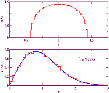
First we consider random network generated by using Erdös and Rényi algorithm. We take nodes and make random connections between pairs of nodes with probability . This method yields a connected network with average degree . Note that for very small value of one gets several unconnected components. Here, the choice of is such that it should be high enough () to give large connected component typically spanning all nodes [33]; and since most of real world networks are very sparse [2], is small enough to have a sparse network. Laplacian is constructed using Eq. (1). Because of the normalized form, the eigenvalues would always be within and . Figure 1(a) plots the spectral density of the Laplacian. Note that the distribution is averaged over 10 realizations of the network. The spectral density follows Wigner-Dyson semicircular distribution [34]. To get the spacing behaviors, first the eigenvalues are unfolded by using the technique described in Sec. 2. This method yields the eigenvalues with constant spectral density on the average. These unfolded eigenvalues are used to calculate NNSD. The same procedure is repeated for an ensemble of the networks generated for different random realizations. Figure 1(b) plots ensemble average of NNSD. By fitting this ensemble averaged NNSD with the Brody formula given in Eq. (3) we get an estimation of the Brody parameter . This value of Brody parameter clearly indicates the GOE behavior of the NNSD [Eq. (2)].
3.2 Scale-free network
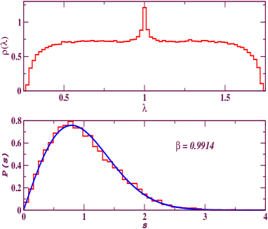
Figure 2 plots the spectral density and the nearest neighbor spacing distribution of the Laplacian of scale-free network. Scale-free network is generated by using the model of Barabási et al. [7]. Starting with a small number, of the nodes, a new node with connections is added at each time step. This new node connects with node with the probability (preferential attachment), where is the degree of the node . After time steps the model leads to a network with nodes and connections. This model leads to a scale-free network, i.e., the probability that a node has degree decays as a power law, , where is a constant and for the type of probability law that we have used . Other forms for the probability are possible which give different values of and we find results similar to the ones reported here. Density distribution of the network has a very uniform distribution for almost all eigenvalues except for few lowest and highest ones. There is a slight peak around which corresponds to the peak at for the adjacency matrix ([21]). To calculate NNSD, we follow same procedure as described in the previous section. Fig. 2(b) shows that spacing distribution of this scale-free network follow GOE very closely .
3.3 Small-world network
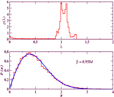
Figure 3 is plotted for small-world network. Small-world networks are constructed using the following algorithm by Watts and Strogatz [8]. Starting with a one-dimension ring lattice of nodes in which every node is connected to its nearest neighbors, we randomly rewire each connection of the lattice with the probability such that self-loop and multiple connections are excluded. Thus gives a regular network and gives a random network. The typical small world behavior is observed around . We take and average degree . Spectral density of this network is complicated with several peaks. One peak is at which corresponds to the peak for the spectra of adjacency matrix. For different values of the exact positions of other peaks may vary but overall form of spectral density remains similar. Fig. 3b) shows that spacing distribution of small world network follows GOE very closely .
Figs. 1(b), 2(b) and 3b) show that spacing distribution of all the three networks follow GOE very closely . Since spectral density of random network is very close to the semicircular, and in RMT literature semicircular distributions are extensively studied and are shown to give GOE statistics of the spacings, we expected that NNSD of random networks would follow as well. But for scale-free network and small-world network, density distributions have very different forms, still NNSD of these networks follow GOE statistics. This is a very interesting result. Following RMT these results imply that even though the spectral density of the scale-free and small-world network differ than the spectral density of the random network, but the correlations among the eigenvalues are strong enough to yield GOE statistics.
4 Transition to GOE statistics and small-world behavior
All the above networks have some amount of random connections in them. In this section we discuss the networks which are regular and analyze the spectral properties as we go from regular network to the random one. Starting with a ring lattice of nodes and average degree , we then randomize some connections with probability , and observe the change in the spectral density and NNSD of the network as a function of . For the original ring lattice, the underlying adjacency matrix would be a band matrix with entries one in the band, except diagonal elements which would be zero. Corresponding Laplacian would be a band matrix as well, with off-diagonal elements (from Eq. (1)), where being the degree of each node, and diagonal elements . As a result of rewiring, few randomly selected pairs of nodes get connected, yielding few nonzero entries outside to the band of the corresponding Laplacian, while making few band elements zero. For a completely random network, the corresponding Laplacian would have non zero random entries.
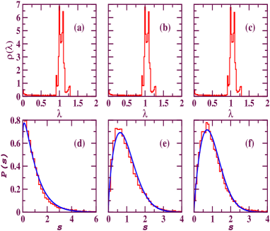
Following we discuss the spectral behavior of Laplacian matrix as number of random connections in the underlying network is increased. Figures 4 (a) and (d) plot density distribution and NNSD for the case. At this value of there is as few as one random rewiring in the regular lattice. These figures shows that spectral density of the lattice is complicated without having any known form; and its spacing distribution closely follows Poisson statistics . We then increase the value of and randomize a fraction of the edges. For this value of , the spectral density and the spacing distribution are plotted respectively in Figure 4 (b) and (e). These figures reveal that for this small value of , density distribution of the network does not show any noticeable change, whereas spacing distribution shows different property (corresponding to the ). As is further increased to the spectral density hardly shows any change but interestingly spacing distribution shows significantly different property than the Poisson statistics. Now the spacing distribution looks more like the intermediate between Poisson and GOE. By fitting the spacing distribution corresponding to this value with the Brody formula, we estimate the Brody parameter as . As marked change in the Brody parameter for very small change in the random connections in the network (corresponding to , Fig. 4 (d)), we had expected that the Brody parameter will reach asymptotically to unity as we increase . But the surprising finding is that the onset of transition from Poisson to GOE occurs at very small value of (Figs. 4 (e) and (f)), and is related with the SW properties of the networks. We calculate the network diameters and clustering coefficients for these values of , which are listed below:
(a) 0.89463 (b) 0.33368 (c) 0.20131
Table 1 shows that for (b) and (c), the average length of the network is as small as the corresponding random network (, and clustering coefficient is as high as the regular lattice (), which are the properties of small-world networks. Values of reveals that Poisson to GOE () transition and small-world transition takes place for the similar value of .
5 Conclusions
In summary, we study eigenvalues spacing distribution of Laplacian of the model networks studied extensively in the literature. They follow universal GOE statistics. From RMT analogy it tells that there exists correlations between the eigenvalues of the network arising from certain symmetries in the interactions. We attribute this universality to the similar amount of randomness in the model networks, which may arise naturally, in order to capture the real world network properties. We study the effect of the randomness in the network connections on the eigenvalues fluctuations of network Laplacian, and use Brody parameter to quantify this randomness. These studies reveal that there is a direct relation between the random connections and the Brody parameter. For the regular network (with the average degree greater then some value) we get Poisson distribution, as we make random rewiring of the connections the spacing distribution start deviating from the Poisson statistics, first it shows intermediate of Poisson and GOE statistics and for sufficiently large number of random connections it show almost GOE statistics (). According to the interpretation of RMT, at this value of , eigenvalues are as much correlated as for the completely random networks. Furthermore we find that this transition to GOE statistics happens at the onset of the small world behavior.
Universal RMT results shown by the networks suggest that they can be modeled as a random matrix chosen from GOE of RMT. Eigenvalues fluctuations following GOE statistics argue that there exists some kind of spreading over the randomness in the whole network, which may be essential for robustness of the system. According to many recent studies, randomness in the connections is one of the most important and desirable ingredients for the proper functionality or the efficient performance of the system having underlying network structure. For instance, information processing in the brain is considered to be highly influenced by random connections among different modular structure [35]. Our analysis suggests that randomness in the complex networks can be studied under the RMT framework. Furthermore, Laplacian spectra have been investigated to understand various dynamical processes on networks [16, 17, 18] as well, hence the RMT analysis of network Laplacians could also be important in view of these demonstrations of the relations between spectral properties and dynamical processes.
Following RMT analysis of adjacency matrices of networks introduced in our previous work [21], we investigate random matrix properties of network Laplacians. In this paper we only concentrate on the spacing distribution of the eigenvalues of the Laplacian, which explains short range correlations among the eigenvalues. Further investigations would involve more sensitive analysis like statistics to understand the long range correlations [36].
6 Acknowledgments
SJ acknowledges Prof. Jürgen Jost for discussing the importance of normalized Laplacians and a very enlighting 2006 summer course in Max-Planck-Institut für Mathematik in den Naturwissenschaften, Leipzig.
References
- [1] S. H. Strogatz, Nature 410, 268 (2001).
- [2] R. Albert and A.-L. Barabási, Rev. Mod. Phys. 74, 47 (2002) and reference therein.
- [3] S. Boccaletti, V. Latora, Y. Moreno, M. Chavez, D.-U. Hwang, Phys. Rep. 424, 175 (2006).
- [4] L. da. F. Costa, F. A. Rodrigues, G. Travieso and P. Villas Boas, Advances in Physics 56, 167 (2007).
- [5] Béla Bollobás, Random Graphs (Second edition, Cambridge Univ. Press, 2001).
- [6] P. Erdös and A. Rényi, Publ. Math. Inst. Hungar. Acad. Sci. 5 17 (1960).
- [7] A.-L. Barabási and R. Albert, Science 286, 509 (1999).
- [8] D. J. Watts and S. H. Strogatz, Nature 440, 393 (1998).
- [9] M. Girvan and M. E. J. Newman, Proc. Natl. Acad. Sci. USA 99, 7821-7826 (2002); A. Clauset, M. E. J. Newman, and C. Moore, Phys. Rev. E 70, 066111 (2004); M. E. J. Newman, Social Networks 27, 39-54 (2005); M. E. J. Newman, Proc. Natl. Acad. Sci. USA 103, 8577-8582 (2006).
- [10] R. Guimerá and L. A. N. Amaral, Nature 433, 895 (2005).
- [11] D. M. Cvetković, M. Doob and H. Sachs, Spectra of Graphs : theory and applications, (Academic Press, 3rd Revised edition, 1997).
- [12] F. R. K. Chung, Spectral Graph Theory, Number 92, AMS (1997).
- [13] Relation between the spectra of and is known only in the case of -regular (degree of each node of the network being equal, ) graphs. In this very special case, , where is a unit matrix, and hence , where and are the eigenvalues spectra of and respectively. For this case, and are linearly related, and therefore the statistical propertes of their spectra would be same. If the degree of nodes are not same, as usually happens in complex networks, then relation between the eigenvalues of and is not known.
- [14] M. Doob in Handbook of Graph Theory, edited by J. L. Gross and J. Yellen (Chapman & Hall/CRC, 2004).
- [15] L. M. Pecora and T. L. Carroll, Phys. Rev. Lett. 80, 2109 (1998); A. E. Motter, Y.-C. Lai and F. C. Hopensteadt, ibid. 91, 014010 (2003); C. Zhou, A. E. Motter and J. Kurths, ibid. 96, 034101 (2006).
- [16] F. M. Atay, T. Biyikoglu, and J. Jost, IEEE Trans. Circuits and Systems I 53, 92, (2006); Physica D 224, 35 (2006).
- [17] P. N. McGraw and M. Menzinger, Phys. Rev. E 75, 027104 (2007).
- [18] D.-H. Kim and A. D. Motter, Phys. Rev. Lett. 98, 248701 (2007).
- [19] R. Grone, R. Merris and V. S. Sunder, SIAM J. Matrix Analysis and Appl. 11, 218 (1990).
- [20] A. Banerjee and J. Jost, Theory in Biosciences 126, 15, (2007).
- [21] J. N. Bandyopadhyay and S. Jalan, Phys. Rev. E, 76, 026109 (2007).
- [22] F. Chung and R. M. Richardson, Quantum Graphs and their Applications, edited by B. Berkolaiko et. al. (Contemporary Math., AMS, Providence, RI, 2006).
- [23] P. Zhu and R. Wilson, in Lecture notes in computer science, Vol. 3691, page 371 (Springer Berlin, 2005); D. Kim and B. Kahng, eprint:arXiv:cond-mat/0703055.
- [24] D. Vukadinovi, P. Huang, T. Erlebach, in Lecture Notes in Computer Science, Vol. 234, page 83 (Springer Berlin, 2002).
- [25] C. Demir, S. H. Gultekin and B. Yener in Proc. of 4th Conference on Modeling and Simulation in Biology, Medicine and Biomedical Engineering (Linkoping, Sweden, May 2005).
- [26] J. Huang, MPI-KYB Technical Report No. 144, available at http://www.cs.uwaterloo.ca/ j9huang/Research/comview.pdf.
- [27] M. L. Mehta, Random Matrices, 2nd ed. (Academic Press, New York, 1991).
- [28] T. Guhr, A. Muller-Groeling and H.A. Weidenmuller, Phys. Rep. 299, 189 (1998).
- [29] V. Pleron, P. Gopikrishnan, B. Rosenow, L. A. N. Amaral, and H. E. Stanley, Phys. Rev. Lett. 83, 1471 (1999).
- [30] P. Seba, Phys. Rev. Lett. 91, 198104 (2003).
- [31] M. S. Santhanam and P. K. Patra, Phys. Rev. E 64,016102 (2001).
- [32] T. A. Brody, Lett. Nuovo Cimento 7, 482 (1973).
- [33] Before this critical value of , one gets several disconnected components. Laplacian matrix of a network having several disconnected components can be written as Kronecker or direct sum of the Laplacian matrices of the disconnected components, i.e., , where is the number of disconnected components. In this case, even if the NNSD of the individual components follows GOE, but in general the NNSD of does not follow GOE property.
- [34] F. Chung, L. Lu and V. Vu, Proc Nat. Acad. Science 100, 6313 (2003).
- [35] J. D. Cohen and F. Tong, Science, 293, 2405 (2001).
- [36] S. Jalan, J. N. Bandyopadhyay and M. S. Santhanam (under preparation).