Marginal intermediate statistics in the excited spectra of E$\otimes(b_{1}+b_{2})$ Jahn-Teller system

Abstract

The long-range spectral density correlations (spectral rigidities $\bar{\Delta}_{3}(\bar{n})$ and related spectral compressibilities) of the $E\otimes(b_{1}+b_{2})$ Jahn-Teller model are found strongly nonuniversal with respect to the Hamiltonian parameters and inhomogeneous with respect to the choice of a partial energy segment. However, the partial spectral rigidities exhibit common features: an anomalous linear part for small $\bar{n}$ and a saturation for large $\bar{n}$. The spectral compressibilities found for the partial spectral segments and averaged over a whole relevant part of the spectrum cumulate close to a well-defined limit pertaining to the semi-Poisson statistics. This is in accordance with similar tendencies revealed in the short-range averaged statistical characteristics of this model investigated in our previous paper (Majerníková and Shpyrko Phys. Rev. E73 057202). These features document an inhomogeneous and nonuniversal weakening of level repulsions and nonuniversality of level fluctuations on both long and short energy scales. The nonuniversality and inhomogeneity of the statistical characteristics correspond to a similar behaviour of the chaoticity parameter (a fraction of the chaotic phase space of the trajectories) found for the corresponding semiclassical Hamiltonian. We ascribe the nonuniversal and inhomogeneous nonintegrability behaviour to the changing degree of the brokening of the rotation symmetry when changing parameters of our effectively two-dimensional model. It results in a random distribution of the respective localized wave functions at all scales up to the size of an available state space. The multifractal behaviour of the wave functions is implied from the analysis of their (averaged) fractal dimensions which range up to $1.5\pm 0.1$ (for $\bar{D}_{2}$). This might imply the concept of the chaos-assisted tunnelling between the regions of reduced degree of stochasticity through regions of high degree of stochasticity. It supports the analogy with the two-dimensional Anderson model with marginal-asymptotically far metal-insulator transition. The features found allow us to classify the present model as a member of the class with a multifractal eigenfunction statistics characteristic for the spectra with weakened level repulsion similar to the Anderson model close to the metal-insulator transition.

1 Introduction

Investigations of a wide class of complex Hamiltonians show a coexistence of ordered and more disconnected chaotic dynamic regions in their phase space in a semiclassical limit [2]. Respective parameters, fractions of the regular and chaotic regions of the phase space were used for the evaluation of statistical characteristics of the related quantum spectra. Namely, explicit formulae for the nearest-neighbour level spacing distributions [3] and the averaged level number variances or the $\Delta_{3}$ statistics [4, 5] were illustrated by a model of two coupled quartic oscillators. The level repulsion at small level spacings was shown to be reduced by the fractionating of the chaotic region which substantially complicated related numerical calculations (level spacing distributions). Discrepancies between the numerical data and the analytical formulae for the above mentioned short-range and also the middle and long-range fluctuation statistics were ascribed especially to quantum effects like the tunnelling between regular regions through chaotic barriers and the quantum interference effects. Finally, the chaos-assisted tunneling approach to the calculation of the level repulsion implied the correct behaviour of the level spacing distributions in the limit of small level separations [6]. This kind of tunnelling was shown to be connected with the fractal dimension of a two-dimensional phase space due to a hierarchical phase space structure of a chaotic system [7].

In this paper, we try to show that one of the systems which exhibit fluctuation properties typical for a transition region between order and chaos with varying (nonuniversal) degree of nonintegrability is the $E\otimes(b_{1}+b_{2})$ Jahn-Teller (JT) model. The model is represented by two degenerate electron levels coupled to two phonon (vibron) modes via two different interaction strengths. Unitary diagonalization of the Hamiltonian in the electron space transforms the system onto two highly nonlinearly coupled quantum oscillators in two dimensions.

In a recent paper [1], we have initiated the study of the statistical evidence of quantum chaotic patterns emerging in this model. We have shown that the (short-range) statistics of the nearest-neighbour level spacings (NNS) in the range of interaction parameters apart from the particular symmetry cases (E$\otimes$e JT and exciton model) is nonuniversal and tends to a well-defined limit close to the semi-Poisson law $P(S)=4S\exp(-2S)$. This intermediate statistics between the Poisson (uncorrelated levels) and the Wigner-Dyson distribution of a correlated fully chaotic level system was found within the frame of random matrix theory as a critical distribution in the metal-insulator transition region in the Anderson model of disorder [8, 9] as well as in several models with not fully developed chaotic dynamics by Bogomolny [10]. Namely, the semi-Poisson distribution of the level spacings in the plasma model was ascribed to the screening (restriction to a finite number of nearest neighbours) of the logarithmic pair interaction potential. Statistical methods for energy levels and eigenfunctions of disordered systems were reviewed by several authors [11].

In section 2, we shall concentrate on the complementary item of the long-range statistics for the excited spectra of the $E\otimes(b_{1}+b_{2})$ JT model with broken rotation symmetry. It comprises the spectral rigidity measure of correlations of the level density on scales large when compared to the mean level spacings. Among possible variants of this measure one can cite the $\bar{\Delta}_{3}$ statistics of Dyson and Mehta [8, 9, 12, 13]. Namely, the $\Delta_{3}$ value is defined as a (random) quantity which for a given energy interval $[-L,L]$ around the value $E_{0}$ gives the deviation of the least-square linear fit line from the staircase function $N(E)$ of the number of levels with energy below $E$:

$$\Delta_{3}(L)={\textrm{min}}_{A,B}\left\{\frac{1}{2L}\int\limits_{-L}^{L}[N(E)-AE-B]^{2}\mathrm{d}E\right\}$$ (1)

(here the energy is shifted so that the interval is centered around $0$; the minimalization is performed with respect to parameters $A,B$). The average of this measure over ensemble $\bar{\Delta_{3}}$ is the quantity of the present interest. The $\bar{\Delta_{3}}$ measure and the correlation function of the level number $\Sigma_{2}(\bar{n})\equiv\langle\delta^{2}N\rangle=\langle N^{2}\rangle-\langle N\rangle^{2}$ (fluctuations of the level number in an energy band of a width $E$, $\bar{n}\equiv\langle N\rangle$ is the length of the energy interval measured by the mean number of the levels inside) are related straightforward as $\bar{\Delta_{3}}(\bar{n})=\frac{2}{\bar{n}^{4}}\int_{0}^{\bar{n}}\left(\bar{n}^{3}-2\bar{n}^{2}r+r^{3}\right)\Sigma_{2}(r)\mathrm{d}r$ [14]. The use of the $\bar{\Delta_{3}}$-statistics instead of the level number fluctuations $\Sigma_{2}$ is justified by the fact that its variance is suppressed when compared to that of $\langle\delta^{2}N\rangle$ [12].

The random matrix theory (RMT) predicts the scaling of this measure as $\log\bar{n}$ (or $\log E$) for the domain of fully developed chaos, meanwhile for the completely uncorrelated sequences of levels a linear scaling $\sim\bar{n}$ is expected [10, 15].

For the Poisson ensemble of an uncorrelated sequence of levels one has $\Sigma_{2}(r)=r$ and $\bar{\Delta}_{3}(\bar{n})=\bar{n}/15$. The number variance $\Sigma_{2}(\bar{n})$ was calculated for a set of ensembles within RMT supposed to model the behaviour of Anderson type systems [15, 16]. Its asymptotic form was shown to be similar to the uncorrelated case but with the coefficient (level compressibility) $\chi<1$, $\Sigma_{2}(\bar{n})\sim\chi\bar{n}$ for large $\bar{n}$. The value $\chi>0$ at weakened level repulsion (compared to the metallic limit) refers to the fractal nature of wave functions. Restricting to the nearest neighbour interactions of the logarithmic pair potential in the Coulomb plasma model Bogomolny et al [10] found the value of the compressibility $\chi=1/2$ which should hold for the models with the semi-Poisson statistics.

In section 3, we discuss a completing semiclassical concept of the degree of chaoticity, i.e., of the phase space fraction occupied by the chaotic trajectories $\mu$ for different segments of the spectra and interaction parameters. A broad region of $\mu$ from increasing to maximum values in the low and middle parts of the spectra to the decreasing again values in the upper parts of the spectra occurs, strongly depending on the parameters and location of the spectral segment. These results confirm the nonuniversality and varying nonintegrability properties as obtained in section 2.

In section 4, an independent quantitative statistical analysis of quantum chaotic patterns of long-range type is provided by the fractal properties of the eigenfunctions: the set of fractal dimensions $D_{q}$ is defined by the scaling properties of the inverse participation ratios $I_{q}(n)$ related to the eigensolution of the state $n$ of a Hamiltonian as $I_{q}(n)=\sum\limits_{r}|\Psi_{n}(r)|^{2q}$. For the sake of application to the excited states of our electron-vibron model (defined in section 2) it is suitable to use the spectral representation where the relevant substrate is the space spanned by the vibron (phonon) Fock states $n$ [17]

$$I_{q}(n)\equiv\sum_{i}|C_{in}|^{2q}.$$ (2)

Here, $C_{in}\equiv\langle\Phi_{i}|\chi_{n}\rangle$; $\chi_{n}(Q_{1},Q_{2})$ are the exact (numerically calculated for the present model) vibron wavefunctions in the space of coordinates $Q_{1}$ and $Q_{2}$; the base set $\Phi_{i}$ is chosen as the set of vibron Fock states - excited states $i$ of the unperturbed two-dimensional harmonic oscillator, namely, $i$ is a compound index denoting the direct product of the excited states $s$ and $t$ of the vibrons $1$ and $2$: $|i\rangle\equiv|s\rangle_{1}\otimes|t\rangle_{2}\sim b_{1}^{{\dagger}s}b_{2}^{{\dagger}t}|0\rangle_{1}\otimes|0\rangle_{2}$.

The scaling with the fractal dimension $D_{q}$ in the spectral representation assumes that one explores the probabilities $P_{i,L}(n)=\sum_{s\in i}P_{s}(n)=\sum_{s}C_{s\in i,n}^{2}$, where the sum is taken over the states inside the cube $i$ of dimension $2$ comprising $l^{2}$ base Fock states and $L$ denotes the number of these cubes ($L\sim 1/l^{2}$). Then,

$$I_{q,L}(n)\propto\sum_{i}^{L}P_{i,L}^{q}(n)\propto L^{-D_{q}(q-1)}\,,$$ (3)

where the information dimension $D_{1}$ is understood as usual in the limit $q\to 1$ as the scaling factor of $\exp(-\sum P_{i}\log P_{i})\propto L^{D_{1}}$. A common assertion found by Kravtsov and Muttalib [18] states that the critical statistics in certain class of systems including Anderson model at M-I transition is in an intimate relation with the weakly overlapping (implying multifractality) wavefunctions.

2 $\bar{\Delta}_{3}$ statistics as a measure of spectral rigidity of the E$\otimes(b_{1}+b_{2})$ Jahn-Teller model

The E$\otimes(b_{1}+b_{2})$ JT model is defined by the Hamiltonian

$$\hat{H}=\Omega(b_{1}^{{\dagger}}b_{1}+b_{2}^{{\dagger}}b_{2}+1)I+\alpha(b_{1}^{{\dagger}}+b_{1})\sigma_{z}-\beta(b_{2}^{{\dagger}}+b_{2})\sigma_{x}$$ (4)

described, e.g., in our previous papers [1, 17, 19]. In short, the local spinless double degenerate electron level is linearly coupled to two intramolecular vibron (phonon) modes of the frequency $\Omega$ by different coupling constants $\alpha\neq\beta$. The pseudospin notation with $2\times 2$ Pauli matrices $\sigma_{x}$, $\sigma_{z}$ and unit matrix $I$ refers to the two-level electron system. The operators $b_{i}$, $b_{i}^{{\dagger}}$ satisfy boson commutation rules $[b_{i},b_{j}^{{\dagger}}]=\delta_{ij}$ and define the vibron coordinates $Q_{i}=\langle b_{i}^{{\dagger}}+b_{i}\rangle$, $i=1,2$. The interaction term $\propto\alpha$ removes the degeneracy of the electron levels and the term $\propto\beta$ mediates the vibron-assisted electron tunnelling between the levels (the class of exciton models differs from the present one by the absence of the vibron-2 assistance in the tunnelling term $\sim\beta$). Two cases of special symmetry comprise the rotation symmetric E$\otimes$e JT model ($\alpha=\beta$) and the polaron model with $\beta=0$ or $\alpha=0$. Introducing nonequal coupling constants the model above generalizes the common E$\otimes$e Jahn-Teller model. The interest for such a generalization has various sources, in particular: (a) different coupling constants are likely to be caused by a spatial anisotropy in a crystal plane; (b) two vibron modes need not have necessary the same frequencies. In this case, the Hamiltonian can be appropriately rescaled to the present model with equal frequencies but different coupling strengths (in what follows we set $\Omega=1$); and, last but not least, (c) the generalized JT system with broken rotational symmetry presents more rich variety of generic chaotic properties than its simpler prototype. As it was shown [1, 17] it stands closer to the generic models of quantum chaotic behaviour.

In the following we use the vibron eigenfunctions of the transformed Hamiltonian $\tilde{H}\equiv U\hat{H}U^{-1}$ [17, 19]

$$\tilde{H}=\Omega(\sum_{i=1,2}b_{i}^{{\dagger}}b_{i}+1)+\alpha(b_{1}^{{\dagger}}+b_{1})-p\beta(b_{2}^{{\dagger}}+b_{2})R_{ph}\,$$ (5)

exactly diagonalized in the electron subspace by the Fulton-Gouterman (FG) unitary operator $U=\frac{1}{\sqrt{2}}\left(\matrix{1\ ,\ R_{ph}\cr 1\ ,\ -R_{ph}}\right),$ where $R_{ph}=\exp(i\pi b_{1}^{{\dagger}}b_{1})$ is the vibron reflection operator imposing high nonlinearity in the system and the parity $p=\pm 1$. It is easy to see that in the FG representation the parities $p=\pm 1$ are exactly mirror images of each other and can be mapped one onto another by a mere change of the sign in the definition of the phonon-2 displacements ($\hat{Q_{2}}\to-\hat{Q_{2}}$), thus the system remains doubly degenerated and the parity does not have any impact on the properties of the spectrum; in what follows we choose $p=+1$.

In the representation of radial coordinates in the plane $Q_{1}\times Q_{2}$, $Q_{1}=r\cos\phi,\ Q_{2}=r\sin\phi$ the transformed Hamiltonian (5) yields [17]

$$\tilde{H}=-\frac{1}{2r}\frac{\partial}{\partial r}\left(r\frac{\partial}{\partial r}\right)+\frac{1}{2}r^{2}-\frac{1}{2r^{2}}\cdot\frac{\partial^{2}}{\partial\phi^{2}}$$

$$+\sqrt{2}\alpha r(\cos\phi-\sin\phi R_{ph})I+p\sqrt{2}(\alpha-\beta)r\sin\phi R_{ph}\,.$$ (6)

The reflection operator $R_{ph}$ in radial coordinates acts as $R_{ph}(r,\phi)f(r,\phi)=f(r,\pi-\phi)$ on some $f(r,\phi)$. An example of the numerical eigenfunction to the transformed Hamiltonian (5) in the space $Q_{1}\times Q_{2}$ is shown in figure 1. Let us note the apparent fractal nature of the space distribution of the state amplitude. The Hamiltonian (6) commutes with the operator of the angular momentum $\hat{J}=i(b_{1}b_{2}^{{\dagger}}-b_{1}^{{\dagger}}b_{2})-\sigma_{y}/2$ if $\alpha=\beta$. Thus, the eigenfunctions of the symmetric model can be chosen each to pertain to a state with a good quantum number $|j|=1/2,3/2,\dots$ [17].

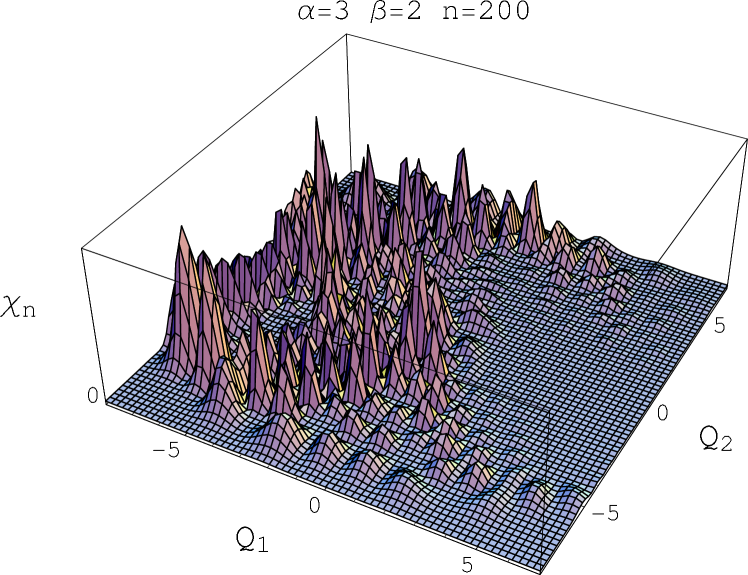
Figure 1: Example of the wavefunction $\chi_{n}(Q_{1},Q_{2})$ for $\alpha=3$, $\beta=2$ and $n=200$.

The last term in (6) breaks the rotational symmetry and involves interactions of the basis states with different $j$. Hence, a wavefunction of the full Hamiltonian is now distributed over a range of values of the angular momentum (figure 2). An analogy to the two-dimensional Anderson model of disorder can be traced if the base functions with definite $j$ are considered as ’pseudosites’ over which the wavefunction is spread. Similarly as in the Anderson model, the properties of the model are determined by the relative strengths of the intersite (different $j$) and the onsite interactions. The microscopic reason for this analogy is the assistance of phonons-2 in transitions between the levels (6) which allows for the emerging of the pseudolattice. To our opinion, it is just these transitions with changing symmetry ($R_{ph}$) which ensured the similarity of the results for NNS distribution [1] to the Anderson model close to the M-I transition (marginal in two-dimensions). Traces of quantum chaos cause the sequence of these coefficients to be distributed in a random fashion with varying $n$ thus supporting the analogy to the Anderson model with a priori given random coefficients.

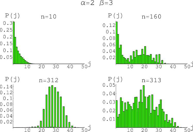
Figure 2: Examples of distributions of wavefunctions over $j$-space for $\alpha=2,\beta=3$. Evidently, the states exhibit different extent of localization.

Calculating the angular part of the matrix elements of the symmetry breaking term in (6) between the states of harmonic oscillator the selection rules can be obtained which assert that the element with definite $j$ is directly connected to the elements with $j^{\prime}=j+2,j-2$ (cf.especially figure 2 with $n=312$ where only every odd ‘pseudosite’ $j$ is populated). This reminds us of an analogy with the ‘daisy models’ of random matrix ensembles [20] with dropping every second term which were shown to lead directly to the semi-Poisson distribution of NNS. The natural ’length’ of our pseudolattice (for a given interval of energy) is thus the maximal number of allowed values of angular momentum for a given n (level number), that is $L\sim\sqrt{n}$ (a state with main quantum number $n_{r}=0,1,\dots$ of a two-dimensional harmonic oscillator is $n_{r}+1$ times degenerated with auxiliary quantum number ranging between $0$ and $n_{r}$, hence $n\sim n_{r}^{2}$). Thus, the analogy to the Anderson type models with M-I transition whose intrinsic characteristics is the length $L$ of a system appears now more pronounced.

In order to calculate the long-range averaged characteristics of the energy spectra of (5) we numerically diagonalized the Hamiltonian matrix in the representation of the base Fock states of the vibrons $1$ and $2$. Taking $N_{1}$ and $N_{2}$ base Fock states for each vibron we introduced an appropriate ordering of sites [21] so that a state vector turned to be a vector with $N_{1}\cdot N_{2}$ elements. Numerical determination of high energy states produces an inevitable error because of truncating the base space. Varying the numbers of the base states we investigated the convergence of the results. For practical purposes we limited ourselves by the base size $N_{1}\times N_{2}=75\times 75$ from whence about 1100-1200 states appeared to be trusty (giving the convergence up to 0.1$\times$(characteristic level spacing)). This number of energy levels was used in the following calculations. Thus, the obtained spectrum needs to be unfolded in order to ensure its homogeneity (that is normalized so that the local averaged level spacing is unity). To do so it is necessary to fit the ’staircase’ $N(E)$ (or the corresponding level density $\rho(E)=\sum_{i}\delta(E-E_{i})$) by a reasonably chosen smooth function. Different choices of the latter are possible. The calculations below used the unfolding by fitting the level density by a third-order spline polynomial (after smoothing the data via Gaussian smoothing with the smoothing constant $0.3$) in the domain of interest, that is for level numbers $100-1200$. In this interval the level density of our two-vibron system grows almost linearly with the energy (we note by passing that this behaviour is in a qualitative accordance with the semiclassical Weyl formula giving generically a linear growth of the level density for a two-vibron system), so that such fitting turns to be more than satisfactory. We performed sample calculations with an increasing order of polynomials, and using other algorithms of producing the smoothed level density $\rho_{sm}$ as well (in particular, varying the parameters of the Gaussian smoothing and using the smoothing via moving average/median); the results appeared indistinguishable within statistical errors.

In order to compile a statistical ensemble out of the (deterministic) quantum problem one has to perform averaging of the numerical quantities of interest over different parts of the spectrum taken as members of this ensemble. We included into the statistical analysis the energy intervals centered at different starting values ranging between 100-1100 levels which corresponded to the energy values between $(-10)$ and $(-5)$ and between $25$ and $30$ depending on the values of ($\alpha,\beta$). However, as it follows from the results below, the ensemble averaged properties can show a bias (sensitivity to the starting point in the energy range), therefore this procedure must be followed with maximal care. To improve the statistics we also followed the standard procedure of collecting statistical data from small intervals in the space of parameters $(\alpha,\beta)$. To be exact, for a given point of interest $(\alpha_{0},\beta_{0})$ we collected the energy values from the square $(\alpha_{0},\beta_{0})\pm 0.25$ in the parameter space with the step $0.1$. (The exception of this rule was collecting the data for the points where $\alpha_{0}=\beta_{0}$. There, this restriction was followed for choosing the neighboring parameters for the sampling). From figure 4 it follows that indeed the averaged statistical data present a slight bias when taking different energy intervals. Therefore we presented the results in figure 4 separately in two energy bins for lower (100-600) and higher (600-1100) levels. It is worth noting that the nonsymmetric parameter values ($\alpha\neq\beta$) appear to present more robust statistics with respect to the energy interval than the symmetric ones ($\alpha=\beta$). The same conclusion was already drawn from the investigation of the short-range statistics [1, 17] where we showed that the spectral properties of the nonsymmetric JT models were more homogeneous with respect to the choice of the energy interval. Taking smaller energy bins than those of figure 4 however did not change much the appearance of the corresponding figures.

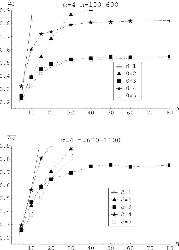
Figure 3: Spectral rigidities ($\bar{\Delta}_{3}$-statistics) in different segments of the spectra for the E$\otimes(b_{1}+b_{2})$ JT model. The slopes are linear for $\bar{n}$ at least up to 15 and tend to nonuniversal saturation values $\bar{\Delta}_{3max}(\beta)$ for large $\bar{n}$.

In figure 3, the samples of the long-range spectral correlations $\bar{\Delta_{3}}$ of the $U$-transformed Hamiltonian (5) (unfolded in a fashion described above) are presented for several sets of interaction parameters. It is seen that the spectral rigidity shows up serious deviations from the Poisson behaviour as well as from the logarithmic dependence expected in the frame of RMT. For large $\bar{n}$ it supposedly tends to a saturation, and a characteristic linear domain is evident for small $\bar{n}$ (up to $\bar{n}\sim 15$).

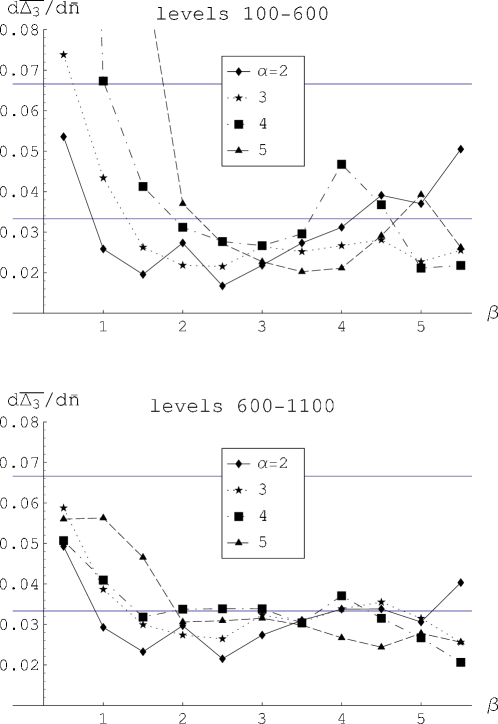
Figure 4: Slopes $\mathrm{d}\bar{\Delta}_{3}(\bar{n})/\mathrm{d}\bar{n}_{|\bar{n}=0}$ (’level compressibilities’) of the long-range statistical measure for different model parameters $(\alpha,\beta)$ for different parts of the spectra. The grid lines indicate the Poisson line (1/15) and the marginal semi-Poisson limit ($\chi=0.5/15\simeq 0.033$). The dispersion of the probability distributions pertaining to the displayed mean values is $\sim 0.01$. The pictures show a strong dependence on the position of the fragment within the spectra.

In figures 4 and 5, we plot the level compressibilities (slopes $\mathrm{d}\bar{\Delta}_{3}(\bar{n})/\mathrm{d}{\bar{n}}_{|\bar{n}=0}$ of the $\bar{\Delta}_{3}$ curves) for a range of parameters $\alpha,\beta$. The slopes in figures 4a, 4b were calculated from averaging over 500 levels in the ranges 100-600 and 600-1100, respectively. Taking lower levels would bring us below the ’diabatic line’ where the system feels only one potential well of the ’effective potential’ (see [19, 17] for a detailed discussion). It is seen from figure 4 that results for different intervals of energy show differences, but, nevertheless, similar tendencies. Apart from the cases close to the special symmetries ($\alpha=\beta$ and $\alpha\ll\beta$, $\alpha\gg\beta$) the slopes show a markable accumulation close to the value $\chi=0.5/15$ (the horizontal grid line at 0.033) indicating the semi-Poisson limit. This limit is more pronounced at higher levels (interval 600-1100), where even the points corresponding to the symmetric cases $\alpha=\beta$ are close to this line. For lower energy interval (levels 100-600) this universality is seen less, although all $\bar{\Delta_{3}}$ curves points are far from both Poisson and RMT limits. For lower energies there is also a more pronounced difference between symmetric and nonsymmetric models: meanwhile the nonsymmetric values of parameters still tend to the semi-Poisson limit, the symmetric points however show essential deviation from this limit towards the Poisson case.

In figure 3, the $\bar{\Delta}_{3}$ curves for $\beta=2,4$ for $\alpha=3$ (scaled by $\Omega=1$) averaged over the whole relevant extent of the spectra (up to the level $n=1100$) are situated very close one to another, i.e. they are getting close to a limit with the minimal slope.

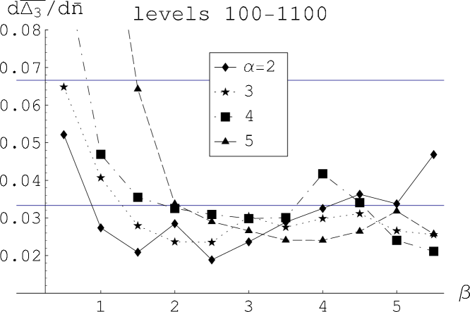
Figure 5: The cumulative slopes $\mathrm{d}\bar{\Delta}_{3}(\bar{n})/\mathrm{d}\bar{n}_{|\bar{n}=0}$ averaged over the relevant extent of the spectra. Large deviation of the points $\alpha=4$, $\beta>4$ from the suggested marginal line is explained by their relative proximity to the symmetric point $\alpha=\beta=4$.

The said marginality also emerged in the statistics of NNS [1]. We have shown that the dispersions $\sigma^{2}$ of NNS distributions in the range of parameters far from the mentioned special symmetry cases tend to a limit $\sigma^{2}\simeq 0.5$ characteristic for the M-I transition of the Anderson model.

3 Quasiclassical description in the phase space

It is interesting to discuss the mapping between the exposed results and the semiclassical description of the same system. The search for the quantum chaotic patterns historically meant looking for quantum correspondence to the chaotic behaviour of the classical trajectories. First of all it is to be noted that the passage to the (semi)classical description in a two- or many-level electron-phonon system can be performed in several fashions. The most straightforward ”semiclassical” description of the quantum JT problem is obtained if we pass to the real Bloch variables made of pseudospin Pauli matrices:

$$x(t):=\langle\sigma_{x}\rangle_{t}\quad y(t):=\langle\sigma_{y}\rangle_{t}\quad z(t):=\langle\sigma_{z}\rangle_{t}$$ (7)

and perform the appropriate decoupling of the oscillatory (phonon) and electron variables in the initial Hamiltonian (4) within the framework of the Born-Oppenheimer approximation: $\langle\hat{Q_{1}}\hat{\sigma_{x}}\rangle\to\langle\hat{Q_{1}}\rangle(t)x(t)$ etc. Another way of passing to the semiclassical description follows from the form of the Hamiltonian (5) where the electron degrees of freedom are exactly eliminated at the cost of the strongly nonlinear coupling of the phonon degrees of freedom. The semiclassical decoupling then means the decoupling of the vibrons 1 and 2. The classical equations of motions in this variant are implied by the following classical Hamiltonian as a function of the coordinates $\gamma_{i}$ and respective momenta $\pi_{i}$:

$$H(\gamma_{1},\pi_{1},\gamma_{2},\pi_{2})=\frac{1}{2}\left[\pi_{1}^{2}+\pi_{2}^{2}+\gamma_{1}^{2}+\gamma_{2}^{2}\right]+\alpha\gamma_{1}\mp\beta\gamma_{2}\exp\left(-2(\gamma_{1}^{2}+\pi_{1}^{2})\right)$$ (8)

The trivial linear stability analysis shows that the stationary point $(\gamma_{1},\gamma_{2},\pi_{1}=\pi_{2}=0)$ is unstable unless $\alpha\gg\beta$, $\alpha\ll\beta$ or unless the parameters ($\alpha,\beta$) are located in the small domain near the point $\alpha=\beta=0$. The crucial characteristics of interest is however the chaoticity of the phase space, in particular, its fraction $\mu$ occupied by the chaotic trajectories. The formulae which relate this quantity to the parameters of the statistics of quantum levels for both short- and long-range statistics are widely known [3, 4, 5]. We investigated the chaoticity of the trajectories implied by the Hamiltonian (8) and performed rough estimations of the ’chaoticity parameter’ $\mu$ for different energies. We studied the sensitivity of the classical equations of motion to the initial conditions checking whether two initially neighboring trajectories diverge in the course of time (that is studying the Lyapunov index [4, 5, 22]). The fraction of the chaotic trajectories at given energy $E$ was then estimated by taking at random the initial points respecting $H(\gamma_{1},\pi_{1},\gamma_{2},\pi_{2})=E$. The detailed quantitative presentation of this work is to be given elsewhere; for the sake of the present contribution we just mention the results briefly. The classical phase space in the energy range corresponding to the energies of quantum levels used (that is up to $E\sim 30$) appears to be pronouncedly chaotic. The fraction of chaotic levels increases rapidly with the increase of energy and reaches its maximum $\mu\sim 0.90-0.99$ for the energies typically $E\sim 10$ which roughly corresponds to the lower energy bin of figure 4 (levels 100-600). With further increasing energy the value of $\mu$ then slowly decreases. Its estimations for $E$ between 20-30 range from $0.3$ to $0.75$ strongly depending on the parameters $\alpha$ and $\beta$. This latter energy interval approximately corresponds to the higher energy bin of figure 4b. We note once again the more pronounced universality of the quantum characteristics at the upper bin (figure 4b) which appears to correspond to the moderate values of the degree of the classical chaoticity. The quantitative conclusions for this item is however a challenge for a separate study.

In any case, the above results confirm the nonuniversal degree of the classical nonintegrability demonstrated by the dependence of the chaoticity parameter $\mu$ on the model parameters $\alpha$ and $\beta$ and on the location of the energy segment in the spectra. Moreover, the linear dependence of the spectral rigidities in certain parts of the spectra implies a strong suppression of the level repulsions because of the presence of regions with various degree of chaoticity and related chaos-assisted tunneling between the regions of small degree of chaoticity. Analogous nonuniversal behaviour of the level compressibilities presented in figure 4 indicates a cumulation of most of their values in the chaotic region $(0,0.033)$ close to the semi-Poisson values $0.5/15$ depending on the spectral segment where the chaoticity parameter is correspondingly reduced.

4 Fractal dimensions and multifractality of the JT-excited wavefunctions

An independent quantitative analysis of the properties of the E$\otimes(b_{1}+b_{2})$ excited spectra can be obtained by exploring the scaling of the inverse participation ratio (2) and (3) in the spectral representation of Fock states and following calculation of related fractal dimensions. In figure 6, we give the samples of the scaling of $\log I_{2,L}(n)$ (from equation (3)) for several successive states as functions of the box size $l$ ($L\sim 1/l^{2}$) comprising $l^{2}$ Fock states. The linear slope in the log-log coordinates stretches up to the box sizes 8$\times$8 which indicates the existence of a well determined quantity $D_{2}$ for each level, although the generalized fractal dimensions show slight level-to-level fluctuations.

Figure 6: Examples of scaling of the inverse participation ratio $I_{2l}(n)$ as a function of the box size $l$ in the box-counting algorithm as the illustration of the reliability of the scaling (3) for our model. Different shapes of symbols correspond to the values for different levels $n$: diamonds for $n=153$, stars for $n=157$, squares for $n=161$. The domain of linear slopes (proportional to the fractal dimensions $D_{2}$) extends up to the box sizes $\sim 8\times 8$ (at larger box sizes the linearity is violated due to the size effects). Slight level-to-level fluctuations of the slopes are also seen. Similar scaling can be demonstrated for $q=3,4$ as well.

In figure 7, the averaged fractal dimensions $\bar{D_{q}}$, $q=1,2,3,4$, in the spectral representation are displayed for a set of interaction strengths. Small variations of $\bar{D_{q}}$ ($\bar{D_{i}}<\bar{D_{j}}$ at $i>j$) testify a weak multifractality of the respective wavefunctions.

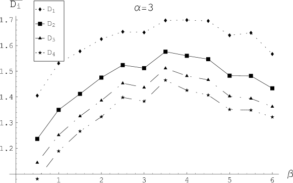
Figure 7: Fractal dimensions $\bar{D_{q}}$ averaged over $n$ for different pairs of $\alpha=3,\beta$. A weak multifractality is evident when comparing $\bar{D_{q}}$ for different $q$.

The fractal dimensions $D_{q}$ show strong fluctuations with changing $n$ (figure 8 so that one has to speak rather about their statistical distributions [23]. It is seen that this distribution may have a pronounced drift – there occurs a crossover between dimensions $d=1$ and $d=2$ at low $n$. It becomes more homogeneous when $n$ increases. In view of the interpretation in terms of the 1D ’pseudolattice’ in $j$-space with natural size of the order $\sim\sqrt{n}$ this can be understood as a tendency towards a universal distribution in the limit of a very large lattice size. Such a limiting behaviour of statistical characteristics of the distribution of fractal dimensions for large lattice sizes of the Anderson model at M-I transition was conjectured by Parshin et al [23].

Figure 8: Fluctuations of fractal dimensions $D_{2}$ over levels $n$ for different pairs $\alpha,\beta$.

Despite the level-to-level fluctuations of the fractal dimensions (figure 8) their values averaged over level numbers appear to exhibit marginal universality in a similar sense as the universality marked in figure 4. The averaged fractal dimensions $\bar{D_{2}}$ in figure 9 show a markable tendency to values $1.5\pm 0.1$ apart from the case $\alpha\gg\beta$ or $\alpha\ll\beta$.

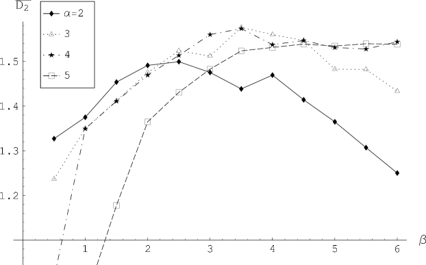
Figure 9: Fractal dimensions $\bar{D_{2}}$ averaged over $n$ in the range 200–400 for different pairs $\alpha,\beta$. In the ’most chaotic’ domain the values of $\bar{D_{2}}$ are distributed in a narrow region $\sim 1.5\pm 0.1$.

5 Conclusion remarks

The statistical properties of the investigated JT model are closely related to its spatial symmetry given by the interaction strengths $\alpha,\beta$. Our numerical analysis of the spectral rigidity, its slopes and fractal dimensions bring the evidence for their apparent nonuniversality and spectral inhomogeneity. Namely, our results allow us to conclude that the nonuniversality is related by the dimensional crossover between $d=1$ and $d=2$ when changing the parameters $\alpha,\beta$. A support for this suggestion is the behaviour of the fractal dimension $\bar{D_{2}}$ (figure 9) which approach very close to the value $1.5$ at the points $\alpha=\beta$. In the neighbourhood of this point the nonuniversality of $\bar{D_{2}}$ is the most moderate; the deviations from $1.5$ extend within the interval $\pm 0.1$.

We have shown that although the long-range correlation measure $\bar{\Delta}_{3}(\bar{n})$ and the partial compressibilities (averaged over partial segments of the spectra) are nonuniversal and highly inhomogeneous, the slopes averaged over the whole relevant spectra approach marginally (quantitatively close) to the universal value characteristic for the semi-Poisson distribution, $0.5/15\sim 0.033$. This behaviour is analogous to the well defined marginal behaviour of the average fractal dimensions $\bar{D}_{2}$ of the respective wavefunctions mentioned above. To our knowledge, till now the theory justifying the existence of the limiting ’universal’ value related to the said distribution is lacking. The only relation $\chi=(d-D_{2})/2d$ derived by Kravtsov and Lerner [15] was the first bridge between the fractal dimension $D_{2}$ and the long-range level statistics. However, it is proven to be valid only for small values of compressibility and does not fit to our calculations.

We have also revealed the corresponding nonuniversal and inhomogeneous behaviour of the chaoticity parameter - the fraction of the chaotic phase space of the classical trajectories. The detailed analysis of this parameter in the whole phase space would be very useful for further considerations of phenomena especially related to the mixing [7] of the phase space between the regions of different degrees of chaoticity. The presence of the mixing phenomena is supported by the multifractal behaviour of the wavefunctions. Because of the nonexistence of the extended states in our model we can conclude on the concept of the chaos-assisted tunnelling between the domains with reduced stochasticity through those with high degree of stochasticity.

Besides the Anderson model close to the metal-insulator transition [8] another models sharing the universal semi-Poisson statistics are known - in particular, the Bogomolny [10] plasma model with screened Coulomb interactions and the ’daisy models’ [20].

References

- [1] Majerníková E and Shpyrko S 2006 Phys. Rev. E73 057202
- [2] Bohigas O, Tomsovic S and Ullmo D, Phys. Rep. 1993 223 43
- [3] Berry M V and Robnik M 1984 J. Phys. A: Math Gen. 17 2413
- [4] Seligman T H and Verbaarschot J J M, J. Phys. A: Math. Gen. 1985 18 2227
- [5] Seligman T H, Verbaarschot J J M and Zirnbauer M R, J. Phys. A: Math. Gen. 1985 18 2751
- [6] Podolskiy V A and Narimanov E E 2003 Phys. Rev. Lett. 91 263601
- [7] Ketzmerick R 1996 Phys. Rev. B 54 10841
- [8] Shklovskii B I, Shapiro B, Sears B R, Lambrianides P and Shore H B 1993 Phys. Rev. B47 11487
- [9] Evangelou S N and Pichard J-L 2000 Phys. Rev. Lett. 84 1643; Evangelou S N and Katsanos D E 2005 Phys. Lett. A 334 331
- [10] Bogomolny E B, Gerland U and Schmit C 1999 Phys. Rev. E59 R1315; Bogomolny E B, Gerland U, and Schmit C 2001 Eur. Phys. J. B 19 121
- [11] Janssen M 1998 Phys. Rep. 295 1; Mirlin A D 2000 Phys. Rep. 326 260
- [12] Dyson F J and Mehta M L 2000 J. Math. Phys. 4 701
- [13] Mehta M L, Nucl. Phys. 1960 18 395; Mehta M L and Gaudin M 1960 Nucl. Phys. 18 420; Gaudin M 1961 Nucl. Phys. 25 447
- [14] Pandey A 1979 Ann. Phys. 119 170
- [15] Kravtsov V E and Lerner I V 1994 Phys. Rev. Lett. 72 888; 1995 Phys. Rev. Lett. 74 2563
- [16] Chalker J T, Kravtsov V E and Lerner I V 1996 Pis’ma v ZhETF 64 355 [1996 JETP Letters 64 386].
- [17] Majerníková E and Shpyrko S 2006 Phys. Rev. E 73 066215
- [18] Kravtsov V E and Muttalib K A 1997 Phys. Rev. Lett. 79 1913
- [19] Majerníková E and Shpyrko S 2003 J. Phys.: Cond. Matter 15 2137
- [20] Hernández-Saldaña H, Flores J and Seligman T H 1999 Phys. Rev. E 60 449
- [21] Życzkowski K, Molinari L and Izrailev F M, J. Phys. I (France) 1994 4 1469
- [22] Benettin G and Strelcyn J M Phys. Rev. A 1978 17 773; Benettin G, Galgani L and Strelcyn J M, Phys. Rev. A 1976 14 2338
- [23] Parshin D A and Schober H R 1999 Phys. Rev. Lett. 83 4590