Irregular Spin Tunnelling for Spin-1 Bose-Einstein Condensates in a Sweeping Magnetic Field

Abstract

We investigate the spin tunnelling of spin-1 Bose-Einstein condensates in a linearly sweeping magnetic field with a mean-field treatment. We focus on the two typical alkali Bose atoms ${}^{87}Rb$ and ${}^{23}Na$ condensates and study their tunnelling dynamics according to different sweeping rates of external magnetic fields. In the adiabatic (i.e., slowly sweeping) and sudden (i.e., fast sweeping) limits, no tunnelling is observed. For the case of moderate sweeping rates, the tunnelling dynamics is found to be very sensitive on the sweeping rates with showing a chaotic-like tunnelling regime. With magnifying the regime, however, we find interestedly that the plottings become resolvable under a resolution of $10^{-4}$ G/s where the tunnelling probability with respect to the sweeping rate shows a regular periodic-like pattern. Moreover, a conserved quantity standing for the magnetization in experiments is found can dramatically affect the above picture of the spin tunnelling. Theoretically we have given a reasonable interpretation to the above findings and hope our studies would bring more attention to spin tunnelling experimentally.

I Introduction

Bose-Einstein condensation (BEC) has been one of the most active topics in physics for over a decade, and yet interest in this field remains impressively high. One of the hallmarks of BEC in dilute atomic gases is the relatively weak and well-characterized interatomic interactions. The vast majority of theoretical and experimental work has involved single component systems, using magnetic traps confining just one Zeeman sublevel in the ground state hyperfine manifold, including the BEC-BCS crossover regal ; zwier , quantized vortices matth ; madison ; raman , condensates in optical lattices greiner , and low-dimensional quantum gases olsh ; gorlitz . An impotent frontier in BEC research is the extension to multicomponent systems, which provides a unique opportunity for exploring coupled, interacting quantum fluids. In particular, atomic BECs with internal quantum structures, some experiments have observed spin properties of $F=1$ and $F=2$ condensates myatt ; stenger ; miesn ; stamp ; chang , using a far-off resonant optical trap to liberate the internal spin degrees of freedom. Even $F=3$ bosons are also investigated in a present theoretical work hoo . For atoms in the $F=1$ ground state manifold, the presence of Zeeman degeneracy and spin-dependent atom-atom interactions stenger ; stamp1 ; barrett ; ho ; law ; pu leads to interesting condensate spin dynamics, especially spin-1 system with its relatively simple internal structure. Many literatures has been devoted to spin mixing and spin domain which had been observed in experiments.

In this article, we investigate spin tunnelling for spin-1 BEC with a mean-field description. Unlike all previous studies of the fixed external magnetic fields both in theory and experiment (e.g., see Refs law ; pu ; wenxian ), we highlight the important role of an external magnetic field that is now set to be linearly varying with time. We focus on the two typical alkali Bose atoms ${}^{87}Rb$ and ${}^{23}Na$ condensates and study their tunnelling dynamics according to different sweeping rates of external magnetic fields. We also pay much attention to a conserved quantity, $m$, standing for magnetization, and find that this quantity can dramatically affects tunnelling dynamics for both ${}^{87}Rb$ and ${}^{23}Na$ atom system.

Our paper is organized as follows. Sec.II introduces our model. In Sec.III we demonstrate our numerical simulations on the irregular spin tunnelling of alkali Bose atoms ${}^{87}Rb$ and ${}^{23}Na$ condensates respectively. In Sec.VI, we present a theoretical interpretation to the above findings with the help of both analytical deductions and phase space analysis. Sec.V is our conclusion.

II The model

In an external magnetic field, spin-1 Bose-Einstein condensate (BEC) is described with the following Hamiltonian wenxian

$$H=\int dr[\psi_{i}^{\dagger}(-\frac{\hbar^{2}}{2M}\nabla^{2}+v+E_{i})\psi_{i}+\frac{c_{0}}{2}\psi_{i}^{\dagger}\psi_{j}^{\dagger}\psi_{j}\psi_{i}+\frac{c_{2}}{2}\psi_{k}^{\dagger}\psi_{i}^{\dagger}(F_{\gamma})_{ij}(F_{\gamma})_{kl}\psi_{j}\psi_{l}],$$ (1)

where repeated indices are summed and $\psi_{i}^{\dagger}(r)$ ($\psi_{i}$) is the field operator that creates (annihilates) an atom in the $i$-th hyperfine state ($\left|F=1,i=+1,0,-1\right\rangle$, hereafter $\left|i\right\rangle$) at location $r$. $M$ is the mass of an atom. Interaction terms with coefficients $c_{0}$ and $c_{2}$ describe, respectively, elastic collisions of spin-1 atoms, expressed in terms of the scattering length $a_{0}$ ($a_{2}$) for two spin-1 atoms in the combined symmetric channel of total spin $0$ ($2$), $c_{0}=4\pi\hbar^{2}\left(a_{0}+2a_{2}\right)/3M$ and $c_{2}=4\pi\hbar^{2}\left(a_{2}-a_{0}\right)/3M$. $a_{0}$ is not spin concerned. $a_{2}$ is spin concerned. $F_{\gamma=x,y,z}$ are spin-1 matrices. Assuming the external magnetic field $B$ to be along the quantization axis ($\widehat{z}$), the Zeeman shift on an atom in state $\left|i\right\rangle$ becomes

$$E_{\pm}=-\frac{E_{hf}}{8}\mp g_{I}\mu_{I}B-\frac{E_{hf}}{2}\sqrt{1\pm\xi+\xi^{2}}$$ (2)

$$E_{0}=-\frac{E_{hf}}{8}-\frac{E_{hf}}{2}\sqrt{1+\xi^{2}}$$ (3)

where $E_{hf}$ is the hyperfine splitting and $g_{I}$ is the Lande $g$ factor for an atom with nuclear spin $I$. $\mu_{I}$ is the nuclear magneton and $\xi=\left(g_{I}\mu_{I}B+g_{J}\mu_{B}B\right)/E_{hf}$ with $g_{J}$ representing Lande $g$ factor for a valence electron with a total angular momentum $J$. $\mu_{B}$ is the Bohr magneton.

At near-zero temperature and when the total number of condensed atoms (N) is large, the system can be well described in the mean-field approximation. For isotropic Bose gas, under the mean-field method and single model approximation, the operators can be substituted with $c$ numbers $\psi_{i}=a_{i}\phi(r)$ where $a_{i}$ correspond to the probability amplitudes of atoms on $i$-th hyperfine state. By setting $a_{i}=\sqrt{s_{i}}e^{i\theta_{i}}$, the system can be described by the following classical Hamiltionian system wenxian ,

$$H_{mf}=E_{+}s_{1}+E_{0}s_{0}+E_{-}s_{-1}-c[(1-s_{1}-s_{-1})^{2}+4s_{1}s_{-1}-4(1-s_{1}-s_{-1})\sqrt{s_{1}s_{-1}}\cos\theta],$$ (4)

where $\theta=\theta_{1}+\theta_{-1}-2\theta_{0}$ and $c=c_{2}\int dr\left|\phi(r)\right|^{4}$. Using canonically conjugate transformation, $H_{mf}$ can be transfered into the following compact classical Hamitonian (up to a trivial constant)

$$H_{c}=2cs_{0}[(1-s_{0})+\sqrt{(1-s_{0})^{2}-m^{2}}\cos\theta]+\delta(1-s_{0}),$$ (5)

and equations of motions for canonically conjugate variables $s_{0}$, $\theta$ are

$$\dot{s_{0}}=\frac{4c}{\hbar}s_{0}\sqrt{(1-s_{0})^{2}-m^{2}}\sin\theta,$$ (6)

$$\dot{\theta}=-\frac{2\delta}{\hbar}+\frac{4c}{\hbar}(1-2s_{0})+\frac{4c}{\hbar}\frac{(1-s_{0})(1-2s_{0})-m^{2}}{\sqrt{(1-s_{0})^{2}-m^{2}}}\cos\theta,$$ (7)

where $m=s_{-1}-s_{1}$ is conserved and denoted as magnetization, and $\delta=(E_{+}+E_{-}-2E_{0})/2$. Fig.1 shows the relationship between $\delta$ and the external magnetic field $B$.

Figure 1: The transformation of $\delta$, expressed in term of the Zeeman shift on an atom in state $\left|i\right\rangle$ ($i=+1,0,-1$) in the external magnetic field $B$. (a) for ${}^{87}Rb$ atom condensate, (b) for ${}^{23}Na$ atom condensate.

III Irregular spin tunnelling

As one of spin dynamics problems, spin tunnelling is always interesting to theoretical and laboratorial investigations. In this section, we study spin tunnelling for the spin-1 BEC systems in a sweeping magnetic field. In our study, the magnetic field varies in time linearly , i.e., $\sim\alpha t$, from $B\rightarrow-\infty$ to $B\rightarrow+\infty$. The sweeping is far away from Feshbach resonance and ensure that the atom-atom interaction is almost not variety during the sweeping process. Numerically, the interval of the magnetic fields is set as $[-B_{0},B_{0}]$ and the $B_{0}$ is chosen larger enough so that the coupling between different components are safely ignored at beginning and ending. In this situation, the spin tunnelling probability can be well defined. We want to know the final value of $s_{0}$ ( i.e. $s_{0}^{Final}$) at $B\rightarrow+\infty(i.e.,B_{0})$, suppose initially we have $s_{0}^{Initial}$ at $B\rightarrow-\infty(i.e.,-B_{0})$. We exploit Runge-Kutta $4^{th}-5^{th}$ algorithm to numerically solve the coupled ordinary differential equations (6) (7) for the parameters corresponding to Bose atoms ${}^{87}Rb$ and ${}^{23}Na$ respectively.

III.1 ${}^{87}Rb$ Atom Condensate

Because ${}^{87}Rb$ atom condensate can be readily prepared in experiments and has been involved in many investigations, we firstly discus it. For convenience and not losing generality, we set the initial probability of $s_{0}$ as $0.5$ for an example. Fig.2 plots the final value of  $s_{0}$ at $B\rightarrow+\infty$, i.e. $s_{0}^{Final}$ for different sweeping rates. The above plotting suggests that our discussions on the spin tunnelling can be divided into three parts according to the values of the sweeping rates $\alpha$.

Figure 2: The tunnelling probability of ${}^{87}Rb$ for $m=0.0,0.1,0.3$ at $c=-3.13\times 10^{-34}J$ in the sweeping magnetic field.

Figure 3: The change of $s_{0}$ (Its initial is $0.5$ at $B\rightarrow-\infty$) with the sweeping magnetic field $B$ for ${}^{87}Rb$ at $m=0.0,0.1,0.3$, $\alpha=1.0,1.01,1.05$ respectively, and $c=-3.13\times 10^{-34}J$.

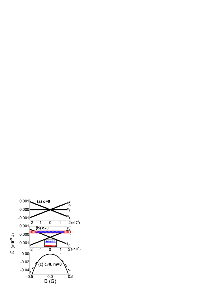
Figure 4: (Color on line) The eigenvalues of ${}^{87}Rb$ atom condensate. (a) is for $c=0$ and different $m$. (b) is for $c=-3.13\times 10^{-34}J$ and differen $m$, where the triangle is $\varepsilon_{2a}$ and the circle is $\varepsilon_{2b}$. The inset shows $\varepsilon_{2a}$ and $\varepsilon_{2b}$ are non-degenerate. (c) is for $c=-3.13\times 10^{-34}J$ and $m=0$, where the dash line is $H_{mf1}$ and the solid line is $H_{mf2}$. To clearly show the spin tunnelling around $B=0$ in fig.3, the unit of horizons of (a) and (b) is taken to be $10^{-6}G$, while it is $G$ in (c).

a) When $\alpha\rightarrow 0$, $s_{0}^{Final}$ almost equal to initial condition $s_{0}=$ $0.5$, as if the system has not been changed. The plotting of tunnelling probability vs. sweeping rates is almost a line, which indicates that no tunnelling occurs after the external magnetic fields sweep slowly from negative infinity to positive infinity. In this case, the system is believed to adiabatically change with the slowly sweeping magnetic field. When the magnetic field changes from $-\infty$ to $+\infty$, $\delta$, the Zeeman shift, changes from an initial value to zero, then returns back to its initial value because of its symmetric dependence on the field (shown in fig.1). Hence, the classical Hamiltonian (5) comes back to origin though the field has been changed dramatically. Numerically solving Eqs.(6, 7) (also see phase space fig.9) we see that for a fixed magnetic field, the motions are periodic. Hence, in light of the adiabatic theoryliuliu , if the sweeping rate of the external magnetic field is small compared to the frequencies of the instantaneous periodic orbits, the the system undergoes adiabatic evolution. Therefore, $s_{0}^{Final}$ $\approx s_{0}.$

b) When $\alpha\rightarrow\infty$, $s_{0}^{Final}$ also tends to $0.5$ (its inital value). The final value of $s_{0}$ oscillates around $0.5$ and tends to a line. In this case, the sweeping rate is so quick, and the system (5) restore quickly. If the time of change the magnetic field is much shorter than the peroid of the motion of system. It is expected that there is no time for the system to give some response to the change of field.  So no tunnelling phenomenon for very fast sweeping rate can also be well comprehended.

c) The interesting phenomena emerge when $\alpha$ is moderate. For this case, we find $s_{0}^{Final}$ changes dramatically with respect to sweeping rates, which indicates spin tunnelling occurs and the tunnelling probability is seemingly chaoticliu . The spin tunnelling process can be shown by drawing the evolution of $s_{0}$ with respect to instantaneous magnetic fields $B.$ In fig.3, we plot the temporal evolution of $s_{0}$ for different sweeping rates $\alpha=1.0,1.01,1.05$ and for each $\alpha$ we choose several magnetization quantities for comparison. From fig.3, one can read that the spin tunnelling happens mainly around $B=0$ regardless of the different quantities of magnetization, and we also see the tunnelling processes are very sensitive on the sweeping rates. Moreover we find the conserved magnetization $m$ dramatically affects the tunnelling processes as well as the final tunnelling probability. For example, in the first row figures of fig.3, with increasing the magnetization from 0 to 0.3, we find that the occupation population of BEC in zero-spin component after a round sweeping of the external magnetic field changes from being enhanced to being quenched compared to its initial state. The influence of the magnetization parameter can be also seen from fig.2, where the fluctuation on the tunnelling probability is clearly suppressed by increasing the value of the magnetization.

The crucial effect of the magnetization parameter on the spin tunnelling can be roughly understood from eqs.(6, 7). It shows that the variation of the population $s_{0}$ is restricted by the conserved magnetization quantity, i.e., $|1-s_{0}|>|m|$.

To explain why the spin tunnelling happens mainly around zero value of the magnetic field, i.e., $B=0$, we calculate the eigenvalues as well as the eigenstates of the system using the similar methods developed in our recent work wang1 . Solving the eigen equations of the system, we obtain the eigenvalues or eigenenergies. Fig.4(a) plots them for linear case, i.e., $c=0$. Fig.4(b) plots them for nonlinear case, i.e., $c\neq 0$. One can see, at $c=0$, the system has three levels. They are $\varepsilon_{1}=E_{+}+c,\varepsilon_{2}=E_{0}+c,\varepsilon_{3}=E_{-}+c$, which cross around $B=0$ and correspond to $m=-1,0,1$ respectively. When $c\neq 0$, the mid-level $\varepsilon_{2}$ is split into two levels, i.e., $\varepsilon_{2a}=\left(E_{+}+E_{-}\right)/2-c$ (the triangles in fig.4(b)) and $\varepsilon_{2b}=E_{0}-c$ (the circles in fig.4(b)) corresponding to $m=\left(E_{+}-E_{-}\right)/4c$ and $m=0$, respectively. $\varepsilon_{2a}$ corresponds to the states of $s_{0}=0$, while $\varepsilon_{2b}$ corresponds to those of $s_{0}=1$. They are seemingly degenerate, while the inset graph in fig.4(b) shows they are actually non-degenerate. Furthermore, we find an interesting phenomenon for this irregular system through investigating the extreme energies of the classical Hamiltonian. After adding the nonlinearity to the system, these extremes are different from the eigenvalues for the same $m$. Taking $m=0$ as an example, in order to ensure the exact position of the extreme energies, we use $H_{mf}$ and obtain its two extreme values $H_{mf1}=E_{0}$, $H_{mf2}=\delta/2+\delta^{2}/16c+E_{0}+c$. They are plotted in fig.4(c). Due to these levels are very close around $B=0$, tunnelling between these levels easily occurs. Moreover, our calculation reveals that these almost degenerate solutions are only emerging in the magnetic field of range $\left[-0.16,0.16\right]G$. It means that the tunnelling should mainly occur in this regime. The above analysis coincide with the jumping regime of $s_{0}$ in fig.3. In this way, we explain why the spin tunnelling mainly happens in a small regime around $B=0$. By the way, from the above analysis we see that in this system the eigenstates do not correspond to the extreme values of energy, e.g., the state of $s_{0}=0.5$ in wenxian is not an eigenstate but a state with an extreme energy. For the same $m$, tunnelling happens between these extreme energies, while the eigenstate on the eigenvalue (e.g., $\varepsilon_{2b}$ in fig.4(b)) is always not change.

Figure 5: The relationship between the initial value of $s_{0}$ at $B\rightarrow-\infty$, $s_{0}^{Initial}$, and its final value at $B\rightarrow+\infty$, $s_{0}^{Final}$, for $\alpha=0.01,0.5,100$, $m=0.0,0.1,0.3$ and $c=-3.13\times 10^{-34}J$.

The above phenomena are general and is independent on the initial condition, namely $s_{0}.$ To more clearly comprehend this point of view, we investigate the relationship between the initial value of $s_{0}$ and $s_{0}^{Final}$. In fig.5, we take $\alpha=0.01,0.5,100$ as an example and calculate the relationship between initial $s_{0}$ and $s_{0}^{Final}$ for several $m$. We see it is a smoothly diagonal line at $\alpha=0.01,100$, which stands for no tunnelling. At $\alpha=0.5$, irregular tunnelling occurs. For the same $\alpha$, the larger $m$, the more smooth the line is, which indicates that $m$ suppresses the irregular tunnelling.

III.2 ${}^{23}Na$ Atom Condensate

${}^{23}Na$ atom condensate has also been prepared in experiments, and its dynamics are also interesting. Different to ${}^{87}Rb$, the interaction between ${}^{23}Na$ atoms is attractive. In this subsection, we will discus its spin tunnelling. In our discussions, we first still take the initial probability of $s_{0}$ as $0.5$ in order to compare with ${}^{87}Rb$ atom condensate. Like the above subsection, our discussions are divided into three parts according to the values of the sweeping rate $\alpha$. The main results are shown in fig.6. We see the tendencies of tunnelling probability for ${}^{23}Na$ atoms are the same as those of ${}^{87}Rb$ atoms. Two little differences are found by comparing the two atom condensates.

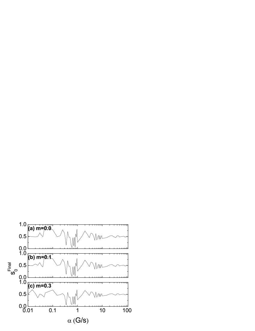
Figure 6: The tunnelling probability of ${}^{23}Na$ for $m=0.0,0.1,0.3$ at $c=3.13\times 10^{-34}J$ in the sweeping magnetic field.

The first difference is the adiabatic range. For ${}^{23}Na$ system, it is smaller than that of ${}^{87}Rb$ system. Because the frequencies of the instantaneous periodic orbits of ${}^{23}Na$ atom system is smaller than those of ${}^{87}Rb$ condensate, the system needs a less sweeping rate to satisfy the adiabatic condition. This difference does not affect the fact of no tunnelling phenomenon at $\alpha\rightarrow 0$. Fig.7 magnifies an adiabatically chaotic-like part of fig.6(a) and shows the above phenomenon. When $\alpha\rightarrow\infty$ and $\alpha$ is moderate, the tunnelling phenomena of ${}^{23}Na$ system are similar to the counterparts of ${}^{87}Rb$ atom system.

The second difference is the effect of the conservation $m$. Like ${}^{87}Rb$ atom condensate, the relationship between $s_{0}^{Final}$ and $s_{0}^{Initial}$ is studied to more clearly understand the irregular spin tunnelling of ${}^{23}Na$ atom condensate. Using the same values of $\alpha$ and $m$ as that in ${}^{87}Rb$ atom system, fig.8 shows the relationship. When the sweeping rate is small, comparing fig.8 with fig.5, we see the lines in fig.5 are smoother than those in fig.8 for a same $\alpha$, such as fig.5(d) and fig.8(d). This indicates that the effect of the conservation $m$ on the spin tunnelling of ${}^{23}Na$ system is less important. When $\alpha$ is moderate, finite value of $m$ suppresses the amplitude of tunnelling probability in fig.8(b)(e)(h) as well as in fig.5(b)(e)(h). The difference is that the amplitude of the fluctuation. This can be seen in fig.6 and fig.2. The suppression effect of the finite magnetization $m$ on the irregularity of tunnelling probabilities for ${}^{23}Na$ system is less significant than that of ${}^{87}Rb$ system. When $\alpha$ is larger, i.e., in the sudden limit, fig.8(c)(f)(i) and fig.5(c)(f)(i) show identical smooth lines without any fluctuations.

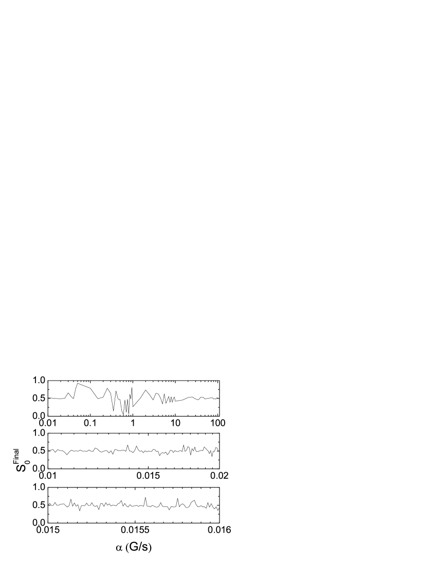
Figure 7: The magnified part of the tunnelling probability of ${}^{23}Na$ at $m=0.0$, $c=3.13\times 10^{-34}J$ in the adiabatic sweeping magnetic field.

Figure 8: The relationship between $s_{0}^{Initial}$ and $s_{0}^{Final}$, for $\alpha=0.01,0.5,100$, $m=0.0,0.1,0.3$ and $c=3.13\times 10^{-34}J$.

IV Interpretation of the irregular spin tunnelling

In this section, we achieve insight into the irregular spin tunnelling effect of spinor BECs with the phase space of the classical Hamiltonian $H_{c}$wang2 . As is discussed above, the tunnelling phenomena of ${}^{23}Na$ and ${}^{87}Rb$ atom condensates have no essential difference. So we take ${}^{87}Rb$ system as an example to interpret the irregular spin tunnelling observed in the above sections.

Fig.9 plots the phase space of Hamilitonian (5) for ${}^{87}Rb$ for different $\delta/c.$ In these phase space we can find two different dynamical regions: (I) running phase region where the relative phase $\theta$ varies monotonically in time; (II) oscillation region where $\theta$ oscillates in time around a fixed point. As $\delta/c$ varies, the areas of these two regions change respectively.

Figure 9: The phase space of ${}^{87}Rb$ for different magnetic field $B$ at $c=-3.13\times 10^{-34}$J, $m=0.0$. The unit of $B$ is Gauss.

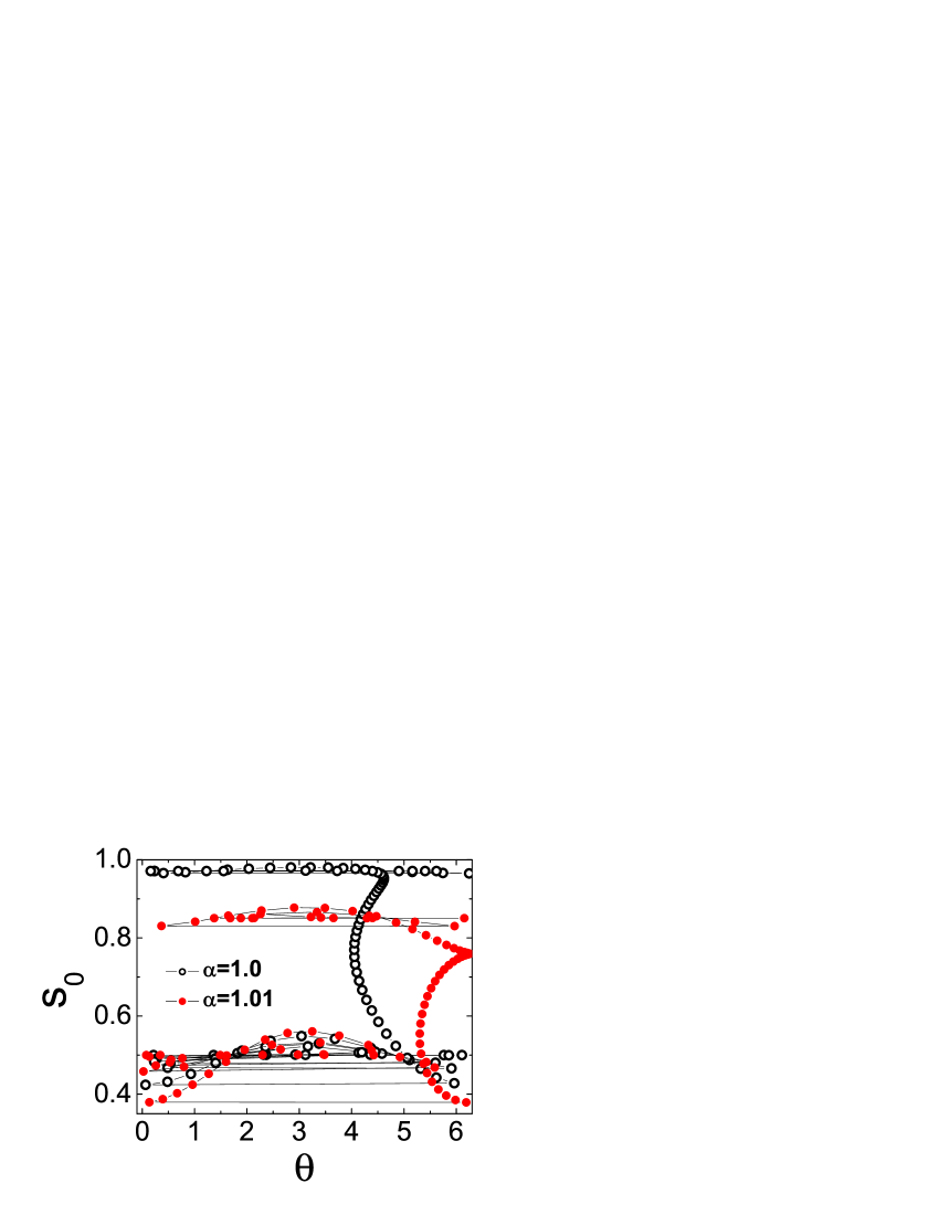
Figure 10: (Color on line) The phase space of ${}^{87}Rb$, which is plotted after an interval of time when the magnetic field moves in an moderate sweeping rate.

At first, $\delta/c\sim\infty,$ all the trajectories are in running phase region. As $B$ changes with a moderate sweeping rate $\alpha$, we record $s_{0},\theta$ after an interval of time and plot them in phase space (see in fig.10). We see that main contribution to the spin tunnelling comes from the transition point where the trajectory passes from the running phase region to the oscillation region or vice versa. For different $\alpha$, the transition point and the final equilibrium place are quite different, for example $\alpha=1.0$ and $\alpha=1.01$ in fig.10. So the tunnelling probabilities are expected to be sensitive on the sweeping rates with showing irregular patterns observed in Fig.5 and 8.

For higher resolution of $\alpha$, the seemingly chaotic tunnelling probability is regular. In fig.11 we plot the magnifying part of fig.2 around $a=1.55$. We find that around a precision $\alpha$ with high resolution the irregular structure becomes the regular one having periodic structure. Set its period is $\alpha_{P}$. When the $\alpha$ is fixed, we find $\alpha_{P}$ has following relation with the initial value of the magnetic field $B_{0}$: $\alpha_{P}\sim 1/\left|B_{0}\right|^{3}$. Fig.12 shows the relationship between $\alpha_{P}$ and $B_{0}$ around $\alpha=1.55$ and $\alpha=2.55$. They are $0.05/\left|B_{0}\right|^{3}$ and $0.15/\left|B_{0}\right|^{3}$ respectively. Furthermore, for a fixed $B_{0}$, the relationship between $\alpha_{P}$ and $\alpha$ is $\alpha_{P}\sim\alpha^{2}$. Fig.13 shows $\alpha_{P}=0.0004,0.0011,0.0022$ around $\alpha=1.55,2.55,3.55$, respectively. We find $0.0004:0.0011:0.0022$ is nicely equal to $1.55^{2}:2.55^{2}:3.55^{2}$. So, the period of regular structure near a sweeping rate is

$$\alpha_{P}\sim\frac{1}{\left|B_{0}\right|^{3}}\alpha^{2}$$ (8)

Figure 11: The magnified part of the tunnelling probability of ${}^{87}Rb$ at $m=0.0$, $c=-3.13\times 10^{-34}J$ in the moderate sweeping magnetic field.

Figure 12: The relationship between $\alpha_{P}$ and $B_{0}$ around $\alpha=1.55$ and $\alpha=2.55$. The dots and the squares are numerical results. The solid line is $\alpha_{P}=0.05/\left|B_{0}\right|^{3}$. The dash line is $\alpha_{P}=0.15/\left|B_{0}\right|^{3}$.

Figure 13: The magnified part of the tunnelling probability of ${}^{87}Rb$ at $m=0.0$, $c=-3.13\times 10^{-34}J$ around $\alpha=1.55,2.55,3.55$ from up to down, respectively.

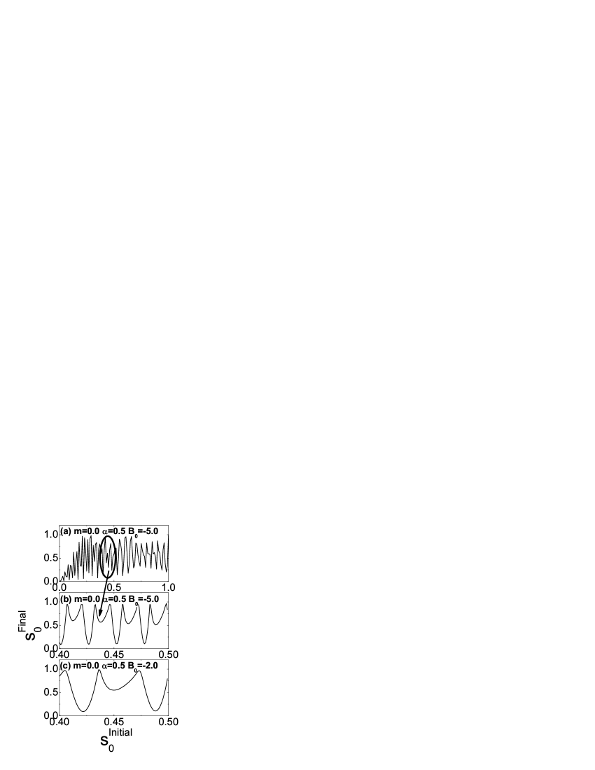
Figure 14: The magnified part of the relationship between $s_{0}^{Initial}$ and $s_{0}^{Final}$ around $s_{0}^{Initial}=0.4$ at $m=0.0$, $c=-3.13\times 10^{-34}J$ in a moderate sweeping magnetic field, i.e., $\alpha=0.5$. (a) is the same as fig.5(b). (b) and (c) are magnified graph of (a) at $B_{0}=-5.0$ and $B_{0}=-2.0$ respectively.

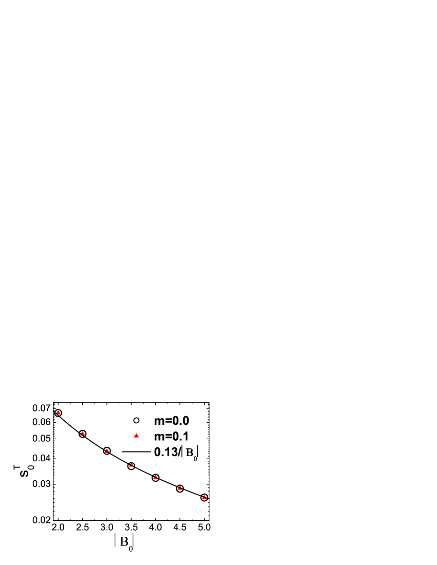
Figure 15: The relationship between $s_{0}^{T}$ and $B_{0}$ around $s_{0}^{Initial}=0.4$. The circles and the triangles are numerical results for $m=0.0,0.1$, respectively, and $\alpha=0.5$. The solid line is $s_{0}^{T}=0.13/\left|B_{0}\right|$.

From this formula, we see that a large $B_{0}$ (used to calculate tunnelling probability in the above section) leads to a small $\alpha_{P}$. If the resolution of the sweeping rates is small compared to the above period, tunnelling probabilities are usually recorded in different period with random phase. So they will looks like chaotic. Only when the resolution is high enough compared to the above period, the regular structure can be observed.

Actually, for a moderate sweeping rate, the chaotic-like relationship between $s_{0}^{Initial}$ and $s_{0}^{Final}$ in fig.5 and 8 is also due to the above reason, that is, when the resolution of the initial values of $s_{0}^{Initial}$ is increased, the observed irregular patterns observed are expected to disappear. Fig.14 shows the magnifying part of fig.5 around $s_{0}^{Initial}=0.4$. Fig.14(b) and fig.14(c) plot this kind of regular structure for different initial magnetic field. Setting the period of this regular structure as $s_{0}^{T}$, we find it satisfy the following relationship between $s_{0}^{T}$ and $B_{0}$: $s_{0}^{T}\sim 1/\left|B_{0}\right|$. In fig.15, this relation is confirmed by our numerical simulations even for different magnetization $m$ and a same $\alpha$. So we expect that the above inversely proportional relation is independent on $m$.

V conclusion

In conclusions, theoretically, we have investigated the tunnelling dynamics of a spin-1 Bose-Einstein condensate in a linearly sweeping magnetic field within a framework of mean field treatment. We focus on the two typical alkali Bose atoms ${}^{87}Rb$ and ${}^{23}Na$ condensates and study their tunnelling dynamics according to different sweeping rates of external magnetic fields. We also investigate the effect of the conserved magnetization on the dynamics of the spin tunnelling. We hope our studies would bring more attention to spin tunnelling experimentally.

VI Acknowledgments

This work was supported by National Natural Science Foundation of China (Grant No.: 10474008,10604009) and by Science and Technology fund of CAEP. We thank Profs. Qian Niu and Biao Wu for stimulating discussions.

References

- (1) LiuJie@iapcm.ac.cn
- (2) C. A. Regal, M. Greiner, and D. S. Jin, Phys. Rev. Lett. 92, 040403 (2004).
- (3) M. W. Zwierlein, C. A. Stan, C. H. Schunck, S. M. F. Raupach, A. J. Kerman, and W. Ketterle, Phys. Rev. Lett. 92, 120403 (2004).
- (4) M. R. Matthews, B. P. Anderson, P. C. Haljan, D. S. Hall, C. E. Wieman, and E. A. Cornell, Phys. Rev. Lett. 83, 2498 (1999).
- (5) K. W. Madison, F. Chevy, W. Wohlleben, and J. Dalibard, Phys. Rev. Lett. 84, 806 (2000).
- (6) C. Raman, J. R. Abo-Shaeer, J. M. Vogels, K. Xu, and W. Ketterle, Phys. Rev. Lett. 87, 210402 (2001).
- (7) M. Greiner, O. Mandel, T. Esslinger, T. W. Hänsch, and I. Bloch, Nature (Lodon) 415, 39 (2002).
- (8) M. Olshanii, Phys. Rev. Lett. 81, 938 (1998).
- (9) A. Görlitz, J. M. Vogels, A. E. Leanhardt, C. Raman, T. L. Gustavson, J. R. Abo-Shaeer, A. P. Chikkatur, S. Gupta, S. Inouye, T. Rosenband, and W. Ketterle, Phys. Rev. Lett. 87, 130402 (2001).
- (10) C. J. Myatt, EA. Burt, R. W. Ghrist, E. A. Cornell, and C. E. Wieman, Phys. Rev. Lett. 78, 586(1997).
- (11) J. Stenger et al, Nature (London) 396, 345(1998).
- (12) H.-J. Miesner et al, Phys. Rev. Lett. 82, 2228(1999).
- (13) D. M. Stamper-Kurn et al, Phys. Rev. Lett. 83, 661(1999).
- (14) M.-S. Chang, C. D. Hamley, M. D. Barrett, J. A. Sauer, K. M. Fortier, W. Zhang, L. You, and M. S. Chapman, Phys. Rev. Lett. 92, 140403(2004).
- (15) Roberto B. Diener and Tin-Lun Ho, Phys. Rev. Lett. 96, 190405(2006).
- (16) D. M. Stamper-Kurn et al, Phys. Rev. Lett. 80, 2027(1998).
- (17) M. Barrett, J. Sauer, and M. S. Chapman, Phys. Rev. Lett. 87, 010404(2001).
- (18) T.-L. Ho, Phys. Rev. Lett. 81, 742(1998).
- (19) C. K. Law, H. Pu, and N. P. Bigelow, Phys. Rev. Lett. 81, 5257(1998).
- (20) H. Pu, C. K. Law, S. Raghavan, J. H. Eberly, and N. P. Bigelow, Phys. Rev. A. 60, 1463(1999).
- (21) Wenxian Zhang, D. L. Zhou, M.-S. Chang, M. S. Chapman, and L. You, Phys. Rev. A. 72, 013602(2005).
- (22) Jie Liu, Biao Wu, and Qian Niu Phys. Rev. Lett. 90, 170404 (2003)
- (23) Jie Liu, Chuanwei Zhang, Mark G. Raizen, and Qian Niu Phys. Rev. A 73, 013601 (2006); Jie Liu, Wenge Wang, Chuanwei Zhang, Qian Niu, and Baowen Li Phys. Rev. A 72, 063623 (2005).
- (24) Guan-Fang Wang, Di-Fa Ye, Li-Bin Fu, Xu-Zong Chen, and Jie Liu Phys. Rev. A 74, 033414 (2006)
- (25) Guan-Fang Wang, Li-Bin Fu, and Jie Liu Phys. Rev. A 73, 013619 (2006)