Boundary-induced bulk phase transition and violation of Fick’s law in two-component single-file diffusion with open boundaries

Abstract

We study two-component single-file diffusion inside a narrow channel that at its ends is open and connected with particle reservoirs. Using a two-species version of the symmetric simple exclusion process as a model, we propose a hydrodynamic description of the coarse-grained dynamics with a self-diffusion coefficient that is inversely proportional to the length of the channel. The theory predicts an unexpected nonequilibrium phase transition for the bulk particle density as the external total density gradient between the reservoirs is varied. The individual particle currents do not in general satisfy Fick’s first law. These results are confirmed by extensive dynamical Monte-Carlo simulations for equal diffusivities of the two components.

I Introduction

One-dimensional exclusion processes belong to the most studied models in non-equilibrium statistical mechanics Ligget85 ; Schu2001 . Their applications are manifold. Among others, the symmetric exclusion process (SEP) plays a role in diffusion where particles, confined in a narrow tube, are not allowed to pass each other Karg92 . This kind of diffusive restriction is referred to as single-file diffusion and differs qualitatively from normal diffusion described by Fick’s law. Whereas in the latter case the mean-square displacement of a single particle grows proportional to time, diffusion is much slower in the single-file case due to mutual blocking of the particles. The mean-square displacement grows (for late times) proportional to the square root of time. The anomalous behaviour of the mean-square displacement usually serves as an experimental indication for the occurrence of single-file diffusion. This requires to trace a single or more particles which implies to label a certain subset of particles without changing the diffusion properties. This corresponds to having a two-species particle system with identical diffusion coefficients Kaerg2002 . Single-file diffusion is a generic phenomenon observed many years ago for molecules diffusing in the channels of certain zeolites Kukla1996 . More recently, single-file behaviour has been demonstrated in the transport of colloidal spheres confined in one-dimensional channels Wei2000 . Moreover confined 1D random motion plays a role in narrow carbon nano tubes, in biological systems like molecular motors or in non-physical systems such as automobile traffic flow Schu2003 . Also the famous repton model by Rubinstein and Duke Rubi87 ; Duke89 ; Bark96 ; Leeuwen2003 for the motion of single polymer chains, is a lattice gas model of this kind. Further motivation for employing single-file diffusion with multiple species comes from recent two-species measurements in zeolites Snurr2002 . Here, a mixture of toluene and propane was adsorbed into different zeolites. The authors measured the temperature dependent outflow and noticed a trapping effect, i.e. in a couple of zeolites the stronger adsorbed toluene molecules influence and control the outflow of propane.

In Keil2000 the authors review the Maxwell-Stefan theory describing the diffusive behaviour of a binary fluid mixture where the total current, i.e. the sum of both species, is zero. The particle-particle interaction is taken into account by including a friction between the species being proportional to the differences in the velocities. This approach does not apply to single-file diffusion in a finite system where, as shown below in the framework of the symmetric simple exclusion process (SEP), the self-diffusivity of single particles plays an important role in the description of the macroscopic behaviour.

The SEP with one species of particles where classical particles with hard-core repulsion diffuse on a finite lattice is well understood Spit70 ; Spoh83 ; vanB83 ; Schu94 ; Ligg99 ; Schu2001 . At both ends the chain is connected to a particle reservoir. One is interested in stationary-state properties like the density profile determined by the reservoir or the stationary particle current as well as the time evolution of the particle density and relaxation towards the stationary state. Our approach for an adequate description of the two-species SEP is a master equation description from which we derive an ansatz of coupled partial differential equations for the macroscopic density profile.

We consider a one-dimensional lattice with $L$ lattice sites (Fig. 1). Each site $i$ can be empty or occupied by a particle of type A or B. Due to hard-core interaction any site carries at most one particle. Particles can hop to nearest neighbour sites (provided the target site is empty) according to the constant hopping rates $D_{A/B}$. Hence, $D_{A}$ ($D_{B}$) is the probability of an A (B) particle to attempt a jump per unit time. The model is defined by random sequential update which forbids simultaneous hopping events. Let $a_{i}$ ($b_{i}$) count the A (B) particles on site $i$. Then the densities are the expectation values of the respective counters: $\left\langle a_{i}\right\rangle\equiv\rho_{A}(i)$, $\left\langle b_{i}\right\rangle\equiv\rho_{B}(i)$. The probability of finding no particle at site $i$ is $\left\langle v_{i}\right\rangle=\left\langle 1-a_{i}-b_{i}\right\rangle$. When we consider a chain with open boundary conditions, particles are injected and removed according to the boundary rates $\alpha_{A/B},\gamma_{A/B},\beta_{A/B}$ and $\delta_{A/B}$, following the notation of Schu2001 . The attempt probability per unit time for an A particle to enter the system at the left boundary is $\alpha_{A}$. It leaves the channel at the left boundary according to $\gamma_{A}$ as illustrated in Fig. 1. The other boundary rates are defined similarly.

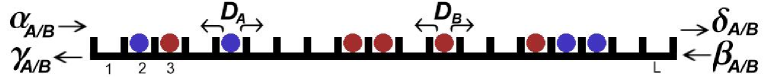
Figure 1: Three-state symmetric exclusion model with open boundaries.

By writing this process in terms of a quantum Hamiltonian formalism Schu2001 , the system evolves in time according to the master equation

$$\frac{d}{dt}|P(t)>=-H|P(t)>$$ (1)

with the generator

$$H=b_{1}+b_{L}+\sum_{i=1}^{L-1}h_{i,i+1}.$$ (2)

For an explicit representation of the generator we denote the state of a given site $i$ by the three basis vectors

$$|A>\equiv|1>=\left(\begin{array}[]{l}1\\ 0\\ 0\end{array}\right),\quad|\emptyset>\equiv|0>=\left(\begin{array}[]{l}0\\ 1\\ 0\end{array}\right),\quad|B>\equiv|-1>=\left(\begin{array}[]{l}0\\ 0\\ 1\end{array}\right)$$ (12)

corresponding to having an A, no particle or B at site $i$, respectively. Let $E_{k}^{x,y}$ be the $3\times 3$ matrix with one element located at column $x$ and row $y$ equal to one. All other elements are zero: $(E_{k}^{x,y})_{a,b}=\delta_{x,a}\delta_{y,b}$. The operator for annihilation (creation) of an A particle at site $k$ is $a_{k}^{-}=E_{k}^{1,2}$ ($a_{k}^{+}=E_{k}^{2,1}$) and for annihilation (creation) of B is $b_{k}^{-}=E_{k}^{3,2}$ ($b_{k}^{+}=E_{k}^{2,3}$). Finally, the number operators are $a_{k}=E_{k}^{1,1}$, $b_{k}=E_{k}^{3,3}$, $v_{k}=1-a_{k}-b_{k}$. This allows to compose the generator of the process. In this representation the boundary matrices are:

$$b_{1}=\alpha_{A}(v_{1}-a_{1}^{+})+\alpha_{B}(v_{1}-b_{1}^{+})+\gamma_{A}(a_{1}-a_{1}^{-})+\gamma_{B}(b_{1}-b_{1}^{-})$$ (13)

$$b_{L}=\delta_{A}(v_{L}-a_{L}^{+})+\delta_{B}(v_{L}-b_{L}^{+})+\beta_{A}(a_{L}-a_{L}^{-})+\beta_{B}(b_{L}-b_{L}^{-})$$ (14)

Hopping in the bulk between site $i$ and $i+1$ occurs according to

$$h_{i,i+1}=D_{A}(a_{i}v_{i+1}+v_{i}a_{i+1}-a_{i}^{-}a_{i+1}^{+}-a_{i}^{+}a_{i+1}^{-})\\ +D_{B}(b_{i}v_{i+1}+v_{i}b_{i+1}-b_{i}^{+}b_{i+1}^{-}-b_{i}^{-}b_{i+1}^{+}).$$ (15)

The model is now well defined. Let us proceed by deriving some equilibrium properties of the process.

II Equilibrium properties

The open system allows for particle exchange at the boundaries. The system is ergodic and will relax to a unique stationary state determined by the boundary rates. The stationary state $|P^{*}>$ does not evolve in time and must obey

$$H|P^{*}>=0.$$ (16)

Let us seek a product ansatz for the equilibrium state of the form

$$|P*>=\left(\begin{array}[]{l}a\\ 1\\ b\end{array}\right)^{\otimes L}\frac{1}{(1+a+b)^{L}}.$$ (20)

The normalization factor of (20) ensures conservation of probability, i.e. ensures that the probability of finding the system in any state is one. Plugging the ansatz (20) into (16) provides a set of equations for the boundary rates and one finds $a=\frac{\alpha_{A}}{\gamma_{A}}=\frac{\delta_{A}}{\beta_{A}}$, $b=\frac{\alpha_{B}}{\gamma_{B}}=\frac{\delta_{B}}{\beta_{B}}$. Taking into account the normalization determines the A and B particle equilibrium densities

$$\rho_{A}=\frac{\frac{\alpha_{A}}{\gamma_{A}}}{1+\frac{\alpha_{A}}{\gamma_{A}}+\frac{\alpha_{B}}{\gamma_{B}}}=\frac{\frac{\delta_{A}}{\beta_{A}}}{1+\frac{\delta_{A}}{\beta_{A}}+\frac{\delta_{B}}{\beta_{B}}}$$ (21)

$$\rho_{B}=\frac{\frac{\alpha_{B}}{\gamma_{B}}}{1+\frac{\alpha_{A}}{\gamma_{A}}+\frac{\alpha_{B}}{\gamma_{B}}}=\frac{\frac{\delta_{B}}{\beta_{B}}}{1+\frac{\delta_{A}}{\beta_{A}}+\frac{\delta_{B}}{\beta_{B}}}.$$ (22)

Besides giving the bulk equilibrium densities, the two equations above provide a recipe of how to translate the picture of inserting and deleting particles on boundary sites into a picture of constant reservoirs at the ends, Fig. 2. In equilibrium the bulk contains no correlations between different lattice sites and the same holds for the boundary and their adjacent sites. Therefore, jumping from a boundary site into the chain occurs proportional to the respective hopping rate and proportional to the single species boundary density. Therefore, given a set of constant boundary rates, Eqs. (21) and (22) define the densities of a virtual particle reservoir at the respective boundaries.

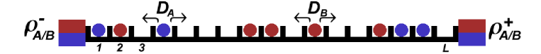
Figure 2: Three-state symmetric exclusion model with open boundaries – reservoir picture.

Note that for this interpretation the left reservoir densities $\rho_{A}^{-}$, $\rho_{B}^{-}$ do not need to be equal to their fellows on the right edge ($\rho_{A}^{+}$, $\rho_{B}^{+}$). In this case the system evolves towards a correlated non-equilibrium stationary state with non-vanishing particle currents. The second and last terms of (21) and (22) are then stationary densities on the left and right edge of the system. This parameterisation satisfies (21) and (22) if

$$\alpha_{A/B}=D_{A/B}\rho_{A/B}^{-},\quad\gamma_{A/B}=D_{A/B}(1-\rho_{A}^{-}-\rho_{B}^{-})$$ (23)

$$\delta_{A/B}=D_{A/B}\rho_{A/B}^{+},\quad\beta_{A/B}=D_{A/B}(1-\rho_{A}^{+}-\rho_{B}^{+}).$$ (24)

III Hydrodynamic limit

The average densities $\left\langle a_{i}\right\rangle$ and $\left\langle b_{i}\right\rangle$ satisfy the equations of motion $\frac{d}{dt}\left\langle a_{i}\right\rangle=-\left\langle a_{i}H\right\rangle$, $\frac{d}{dt}\left\langle b_{i}\right\rangle=-\left\langle b_{i}H\right\rangle$ (cf. Schu2001 ). This provides the Master equations for a single site,

$$\frac{d}{dt}\left\langle a_{i}\right\rangle =D_{A}\left(\left\langle a_{i-1}v_{i}\right\rangle+\left\langle a_{i+1}v_{i}\right\rangle-\left\langle a_{i}v_{i+1}\right\rangle-\left\langle a_{i}v_{i-1}\right\rangle\right)$$ (25)

$$\frac{d}{dt}\left\langle b_{i}\right\rangle =D_{B}\left(\left\langle b_{i-1}v_{i}\right\rangle+\left\langle b_{i+1}v_{i}\right\rangle-\left\langle b_{i}v_{i+1}\right\rangle-\left\langle b_{i}v_{i-1}\right\rangle\right).$$ (26)

From now on we discuss the case of equal hopping rates $D_{A}=D_{B}=D$. Imagining the individual particle species $A$ and $B$ to be distinguishable by a “colour” (in an abstract sense) we shall refer to the total particle density (averaged over $A$ and $B$ particles) as colourblind density.

Let us first assume an infinite system and do not care about boundary sites. But still, in this form the equations of motion are not integrable. Replacing the joint probabilities by products of expectation values, according to a mean field ansatz which has been proven to be useful in other systems, fails. However, an exact equation containing no correlators can be achieved from a sum of both

$$\frac{d}{dt}\left(\left\langle a_{i}\right\rangle+\left\langle b_{i}\right\rangle\right)=D\left(\left\langle a_{i-1}\right\rangle+\left\langle a_{i+1}\right\rangle-2\left\langle a_{i}\right\rangle+\left\langle b_{i-1}\right\rangle+\left\langle b_{i+1}\right\rangle-2\left\langle b_{i}\right\rangle\right).$$ (27)

The right-hand side contains a second-order difference for both species individually. (27) is the discrete analogue of the diffusion equation for the colourblind macroscopic profile. Introducing a lattice constant $a$ and replacing $i$ by the continuous variable $x=\frac{i}{a}$, transforms (27) for the hydrodynamic limit of vanishing lattice constant $a$ into

$$\partial_{t}\left(\rho_{A}(x,t)+\rho_{B}(x,t)\right)=D\partial_{x}^{2}(\rho_{A}(x,t)+\rho_{B}(x,t)).$$ (28)

for the macroscopic particle densities $\rho_{A}(x,t)$, $\rho_{B}(x,t)$.

Following the argument of Quastel we make an ansatz for the dynamics of a single particle localized at position $x$. For a short-time region this particle acts as a tracer particle in the background of other particles with the self-diffusion coefficient $D_{S}(x,t)$. Going beyond Quastel we argue that for the finite-size problem with open boundaries $D_{S}$ is given by expression

$$D_{S}=D\frac{1-\rho_{A}-\rho_{B}}{\rho_{A}+\rho_{B}}\frac{1}{L}.$$ (29)

derived originally for a periodic lattice vanB83 . Additionally, the test particle is subjected to a drift $b$ caused by the evolution of the entire system towards its stationary state. For a good intermixed background one would expect the drift velocity $b$ to be the same for both species of particles. We thus arrive at the ansatz

$$\partial_{t}\rho_{A}(x,t) =\partial_{x}^{2}D_{S}\rho_{A}(x,t)-\partial_{x}b\rho_{A}(x,t)$$ (30)

$$\partial_{t}\rho_{B}(x,t) =\partial_{x}^{2}D_{S}\rho_{B}(x,t)-\partial_{x}b\rho_{B}(x,t).$$ (31)

The self-diffusion coefficient $D_{S}$ as well as the drift $b$ are functions of $\rho_{A}$ and $\rho_{B}$ and hence, depend implicitly on $x$ and $t$. The drift term can be determined by using the colourblind exact result (28) and one finds

$$b=\frac{1}{\rho}\partial_{x}\left[\rho(D_{S}-D)\right].$$ (32)

This completes the hydrodynamic description of the two-component symmetric exclusion process with open boundaries that we propose. A derivation of $D_{S}$ on a finite lattice with two different particle species Brz06 will be presented in a forthcoming paper Brza07 .

IV Stationary state

It is a significant property of particle systems with open boundaries that they can relax to a steady state with non-vanishing particle currents. The stationary state of the colour-blind profile $\rho=\rho_{A}+\rho_{B}$ is linear with the slope being determined by the sum of the boundary densities on the left ($\rho^{-}=\rho_{A}^{-}+\rho_{B}^{-}$) and on the right edge ($\rho^{+}=\rho_{A}^{+}+\rho_{B}^{+}$) of the system which is manifest by (28),

$$\rho=\rho^{-}+\left(\rho^{+}-\rho^{-}\right)\frac{x}{L}.$$ (33)

Integrating (30) once for vanishing time derivative yields

$$\frac{d}{dx}\rho_{A}+\left(\frac{D}{D_{S}}-1\right)\frac{\rho^{\prime}}{\rho}\rho_{A}+\frac{j_{A}}{D_{S}}=0.$$ (34)

where $j_{A}$ is the constant $A$-particle current. Absorbing $\rho_{A}^{-}$ into the integration constant yields the solution

$$\rho_{A}(x)=\frac{\rho(x)}{\rho^{-}}\left[-\frac{Lj_{A}\rho^{-}}{D(\rho^{+}-\rho^{-})}+\left(\rho_{A}^{-}+\frac{Lj_{A}\rho^{-}}{D(\rho^{+}-\rho^{-})}\right)\left(\frac{1-\rho(x)}{1-\rho^{-}}\right)^{L}\right]\quad\rho^{+}\neq\rho^{-}.$$ (35)

The first term is linear in $x$ and describes the bulk region. The nonlinear second term describes a boundary layer, first observed numerically in the Rubinstein-Duke model Leeuwen2003 for different boundary rates. Our analysis shows that the length of the boundary layer does not scale with system size. This can be seen by rewriting (35) for sufficiently large $L$ and assuming $\rho^{+}>\rho^{-}$:

$$\rho_{A}(x)=\left(1+\frac{\rho^{+}-\rho^{-}}{\rho^{-}}\frac{x}{L}\right)\left(-\frac{Lj_{A}\rho^{-}}{D(\rho^{+}-\rho^{-})}+\left(\rho_{A}^{-}+\frac{Lj_{A}\rho^{-}}{D(\rho^{+}-\rho^{-})}\right)e^{-\frac{\rho^{+}-\rho^{-}}{1-\rho^{-}}x}\right)\quad\rho^{+}>\rho^{-}$$ (36)

The localization length

$$\xi=\frac{1-\rho^{-}}{\rho^{+}-\rho^{-}}$$ (37)

does not depend on the system size. In the limit of infinite $L$ the relative size of the boundary layer vanishes and the linear solution connects to the reservoir densities by a jump discontinuity at one of the edges. For $\rho^{+}>\rho^{-}$ the exponential in (36) dominates for small $x$ and the discontinuity is located on left boundary. The case $\rho^{+}<\rho^{-}$ is similar, but the discontinuity is at the right edge.

The case of equal reservoir densities $\rho_{+}=\rho_{-}=\rho$ has to be treated separately. The self-diffusion coefficient is constant, hence, the $b$ in (30) vanishes. Integrating (30) with $\rho_{A}(0)=\rho_{A}^{-}$ yields the linear density profile

$$\rho_{A}(x)=\rho_{A}^{-}+\left(\rho_{A}^{+}-\rho_{A}^{-}\right)\frac{x}{L}$$ (38)

and a similar expression for the density of $B$-particles.

Fig. 3 shows the A and B particle densities obtained from Monte Carlo simulations (symbols) and the theoretical stationary state solutions (solid lines). The explicit expressions for the particle currents are given below. We apply the same set of reservoir densities $\rho_{A}^{-}=\rho_{B}^{-}=1/3$, $\rho_{B}^{+}=\frac{e}{1+e^{-1}+e}$ and $\rho_{A}^{+}=\frac{e^{-1}}{1+e^{-1}+e}$ used in Fig. 9 of Leeuwen2003 . This choice is motivated by boundary rates used in the Rubinstein-Duke model for describing the tensile force acting at the chain ends of reptating polymers. The different lattice sizes a) $L=50$ and b) $L=200$ demonstrate the finite-size character of the boundary layer. The theoretical solution does not contain an inflection point and deviates slightly from simulations in the immediate vicinity of the boundary. Nevertheless, an interesting observation captured by the theoretical description is confirmed. The solution has a minimum in the density profile (although not very pronounced in the sample A-profile of Fig. 3) and, hence, as in the Rubinstein-Duke model there exists a region where one of the particle currents does not follow the direction of the density gradient.

Figure 3: Stationary state with finite slope of the colour-blind density. a) $L=50$, b) $L=100$. The boundary densities are $\rho_{A}^{-}=\rho_{B}^{-}=1/3$, $\rho_{A}^{+}=\frac{e}{1+e^{-1}+e}$ and $\rho_{A}^{+}=\frac{e^{-1}}{1+e^{-1}+e}$.

We conclude by analyzing the behaviour of the current and the mean particle density in the system. Using (35), (38) and taking into account the A particle reservoir density on the right edge gives the current

$$j_{A}=\begin{cases}-\frac{D(\rho^{+}-\rho^{-})}{L}\frac{\frac{\rho_{A}^{+}}{\rho^{+}}-\frac{\rho_{A}^{-}}{\rho^{-}}\left(\frac{1-\rho^{+}}{1-\rho^{-}}\right)^{L}}{1-\left(\frac{1-\rho^{+}}{1-\rho^{-}}\right)^{L}}&\rho^{+}\neq\rho^{-}\\ -\frac{D}{L^{2}\rho}(\rho_{A}^{+}-\rho_{A}^{-})(1-\rho)&\rho^{+}=\rho^{-}\end{cases}$$ (39)

This has an interesting consequence. Considering large $L$ (39) simplifies asymptotically to

$$j_{A}=\begin{cases}-\frac{D}{L}\frac{(\rho^{+}-\rho^{-})\rho_{A}^{+}}{\rho^{+}}&\rho^{+}>\rho^{-}\\ -\frac{D}{L}\frac{(\rho^{+}-\rho^{-})\rho_{A}^{-}}{\rho^{-}}&\rho^{+}<\rho^{-}\\ -\frac{D}{L^{2}\rho}(\rho_{A}^{+}-\rho_{A}^{-})(1-\rho)&\rho^{+}=\rho^{-}.\end{cases}$$ (40)

Hence, provided a finite slope of the colour-blind profile, the individual particle currents are proportional to $1/L$, as for the single-component case, whereas for $\rho^{+}=\rho^{-}$ the currents vanish proportional to $1/L^{2}$.

We make an interesting observation if the relation $\rho_{A}^{-}\rho_{B}^{+}=\rho_{A}^{+}\rho_{B}^{-}$ is satisfied. For this particular case the individual density profiles are linear and the particle currents are just proportional to the respective density gradients (Fick’s law). If the relation does not apply we observe a boundary layer inside which the current flows against the local gradient. Here Fick’s law is violated.

Finally, the mean $A$-density in the channel can be obtained by integrating (36). Asymptotically for large $L$ one finds from (40)

$$\overline{\rho_{A}}=\begin{cases}\frac{\rho_{A}^{+}(\rho^{-}+\rho^{+})}{2\rho^{+}}&\rho^{+}>\rho^{-}\\ \frac{\rho_{A}^{-}(\rho^{-}+\rho^{+})}{2\rho^{-}}&\rho^{+}<\rho^{-}\\ \frac{\rho_{A}^{-}+\rho_{A}^{+}}{2}&\rho^{+}=\rho^{-}.\end{cases}$$ (41)

The mean $A$-density evaluated as a function of the boundary densities may have a discontinuity. Assume $\rho^{-}$ and $\rho_{A}^{-}\neq\rho_{A}^{+}$ be fixed. When taking the limit $\rho^{+}\to\rho^{-}$ coming from small $\rho^{+}$ the total density approaches $\overline{\rho_{A}}\to\rho_{A}^{-}$. Taking the limit from the other site, $\overline{\rho_{A}}\to\rho_{A}^{+}$. There is a jump of the mean $A$-density when the colour-blind boundary densities become equal. Since the colour-blind density is the sum of $A$ and $B$ densities, this implies a jump discontinuity also in the mean $B$-density. Therefore there is a first-order nonequilibrium phase transition in this boundary-driven lattice gas model for two-component single-file diffusion. Such a transition is not known for boundary-driven one-component systems.

Acknowledgement: Financial support by the Deutsche Forschungsgemeinschaft is gratefully acknowledged. We also thank Rosemary Harris, Jörg Kärger and Henk van Beijeren for useful discussions.

References

- (1) T. M. Liggett, Interacting Particle Systems, Springer, New York (1985).
- (2) G. M. Schütz, in Phase Transitions and Critical Phenomena 19, 1, C. Domb and J. Lebowitz (eds.), Academic Press, London 2001.
- (3) J. Kärger and D.M. Ruthven, Diffusion in Zeolites and Other Microporous Solids, Wiley: New York 1992.
- (4) S. Vasenkov, J. Kärger, Phys. Rev. E 66 (2002) 052601.
- (5) V. Kukla, J. Kornatowski, D. Demuth, I. Girnus, H. Pfeifer, L. V. C. Rees, S. Schunk, K. Unger and J. Kärger, Science 272 (1996) 702.
- (6) Q-H. Wei, C. Bechinger and P. Leiderer, Science 287 (2000) 625.
- (7) G. M. Schütz, J. Phys. A 36 (2003) R339
- (8) M. Rubinstein, Phys. Rev. Lett. 59 (1987) 1946.
- (9) T.A.J. Duke, Phys. Rev. Lett. 62 (1989) 2877.
- (10) G.T. Barkema and G.M. Schütz, Europhys. Lett. 35, 139 (1996).
- (11) A. Drzewinski, E. Carlon, J. M. J. van Leeuwen, Phys. Rev. E 68 (2003) 061801.
- (12) K. F. Czaplewski, T. L. Reitz, Y. J. Kim, R. Q. Snurr, Micropor. Mesopor. Materials, 56 (2002) 55.
- (13) F. Keil, R. Krishna, M.-O. Coppens, "Modeling of diffusion in zeolites", Rev. Chem. Eng. 16 (2000)
- (14) F. Spitzer, Adv. Math. 5 (1970) 246.
- (15) H. Spohn, J. Phys. A 16 (1983) 4275.
- (16) H. van Beijeren, K. W. Kehr, R. Kutner, Phys. Rev. B 28 (1983) 5711.
- (17) G. Schütz, S. Sandow, Phys. Rev. E 49 (1994) 2726.
- (18) T.M. Liggett: Stochastic Interacting Systems: Contact, Voter and Exclusion Processes (Springer, Berlin, 1999).
- (19) J. Quastel, Comm. Pure Appl. Math. 45 (1992) 623-679.
- (20) A. Brzank, Molecular traffic control and single-file diffusion with two species of particles, PhD Thesis, Universitaet Leipzig.
- (21) A. Brzank, D. Karevski and G.M. Schütz, unpublished.