The Asymmetric Simple Exclusion Process : An Integrable Model for Non-Equilibrium Statistical Mechanics

Abstract

The Asymmetric Simple Exclusion Process (ASEP) plays the role of a paradigm in Non-Equilibrium Statistical Mechanics. We review exact results for the ASEP obtained by Bethe Ansatz and put emphasis on the algebraic properties of this model. The Bethe equations for the eigenvalues of the Markov Matrix of the ASEP are derived from the algebraic Bethe Ansatz. Using these equations we explain how to calculate the spectral gap of the model and how global spectral properties such as the existence of multiplets can be predicted. An extension of the Bethe Ansatz leads to an analytic expression for the large deviation function of the current in the ASEP that satisfies the Gallavotti-Cohen relation. Finally, we describe some variants of the ASEP that are also solvable by Bethe Ansatz.

I Introduction

Equilibrium statistical mechanics tells us that the probability of a microstate of a system in equilibrium with a thermal reservoir is given by the Boltzmann-Gibbs law : if ${\mathcal{H}}$ is the Hamiltonian of the system, the probability distribution over the configuration space is proportional to $\exp(-\beta{\mathcal{H}})$ where $\beta$ is the inverse of temperature. This canonical prescription is the starting point for any study of a system in thermodynamic equilibrium : it has provided a firm microscopic basis for the laws of classical thermodynamics, has allowed us to describe various states of matter (from liquid crystals to superfluids), and has led to a deep understanding of phase transitions that culminated in the renormalisation group theory.

For a system out of equilibrium, the probability of a given microstate evolves constantly with time. In the long time limit such a system may reach a stationary state in which the probability measure over the configuration space converges to a well-defined and constant distribution. If the system carries macroscopic stationary currents that represent interactions and exchanges of matter or energy with the external world, this stationary distribution is generically not given by the canonical Boltzmann-Gibbs law. At present, there exists no theory that can predict the stationary state of a system far from equilibrium from a knowledge of the microscopic interactions of the elementary constituents of the system amongst themselves and with the external environment, and the dynamical rules that govern its evolution. The search for general features and laws of non-equilibrium statistical mechanics is indeed a central topic of current research.

For systems close to thermodynamic equilibrium, linear-response theory yields the fluctuation-dissipation relations and the Onsager reciprocity relations. However, these properties of non-equilibrium statistical mechanics are only valid in the vicinity of equilibrium. Another route to explore and discover the characteristics of a general theory for systems out of equilibrium is through the study of mathematical models. These models should be simple enough to allow an exact and thorough mathematical analysis, but at the same time they must exhibit a complex phenomenology and must be versatile enough to be of physical significance. In the theory of phase transitions such a corner-stone was provided by the Ising model. It is natural to expect that a well-crafted dynamical version of the Ising model could play a key role in the development of non-equilibrium statistical mechanics. Driven lattice gases (Katz, Lebowitz and Spohn 1984; for a review see Schmittmann and Zia, 1995) provide such models; they represent particles hopping on a lattice and interacting through hard-core exclusion. The particles are subject to an external field that induces a bias in the hopping rates resulting in a stationary macroscopic current in the system. Due to this current, the microscopic detailed balance condition is violated and the system is generically in a non-equilibrium stationary state.

The Asymmetric Simple Exclusion Process (ASEP) in one dimension is a driven lattice gas that can be viewed as a special case of the general class of models defined by Katz, Lebowitz and Spohn. This stochastic particle system was simultaneously introduced as a biophysical model for protein synthesis on RNA (MacDonald and Gibbs 1969) and as a purely mathematical tool for the study of interaction of Markov processes (Spitzer 1970, Liggett 1985, Spohn 1991, Liggett 1999). Subsequently, the ASEP has been used to study a wide range of physical phenomena : hopping conductivity in solid electrolytes (Richards 1977), transport of Macromolecules through thin vessels (Levitt 1973), reptation of polymer in a gel (Widom et al. 1991), traffic flow (Schreckenberg and Wolf 1998), surface growth (Halpin-Healy and Zhang 1995, Krug 1997), sequence alignment (Bundschuh 2002) and molecular motors (Klumpp and Lipowsky, 2003).

From a theoretical point of view, the ASEP plays a fundamental role in the study of non-equilibrium processes (Krug 1991). Many exact results for the ASEP have been derived using two complementary approaches, the Matrix Product Ansatz and the Bethe Ansatz (for a review see Derrida 1998, Schütz 2001), the relation between these two Ansätze being still a matter of investigation (Stinchcombe and Schütz 1995; Alcaraz and Lazo 2004).

The Matrix Product Ansatz, inspired from the quantum inverse scattering method (Faddeev 1984), is based on a representation of the components of the steady state wave function of the Markov operator in terms of a product of non-commuting operators. This Matrix Product technique, initially introduced for the ASEP with open boundaries (Derrida et al. 1993), has proved to be a very efficient tool to calculate steady state properties such as equal time correlations in the steady state, current fluctuations (Derrida et al. 1997), and large deviation functionals (Derrida et al. 2003). This technique has been used to prove rigorously that the invariant distribution of the ASEP with two classes of particles is not a Gibbs measure (Speer 1993).

The second approach, which consists in applying the Bethe Ansatz to a non-equilibrium process such as the ASEP, is due to D. Dhar (1987). The Markov matrix that encodes the stochastic dynamics of the ASEP can be rewritten in terms of Pauli matrices; in the absence of a driving field, the symmetric exclusion process can be mapped exactly into the Heisenberg spin chain. The asymmetry due to a non-zero external driving field breaks the left/right symmetry and the ASEP becomes equivalent to a non-Hermitian spin chain of the XXZ type with boundary terms that preserve the integrable character of the model. The ASEP can also be mapped into a six vertex model (Baxter 1982, Kandel et al., 1990). These mappings suggest the use of the Bethe Ansatz to derive spectral information about the evolution operator, such as the spectral gap (Gwa and Spohn 1992, Kim 1995, Golinelli and Mallick 2004a, 2005a) and large deviation functions (Derrida and Lebowitz 1998; Derrida and Appert 1999; Derrida and Evans 1999).

The aim of the present work is to provide the reader with an introduction to integrability methods applied to the ASEP and to describe some of the exact results derived with the help of the Bethe Ansatz. Our presentation assumes little prior knowledge of these methods and we put emphasis on the algebraic properties of the model. In fact, the ASEP on a periodic ring is one of the most elementary systems to which the Bethe Ansatz can be applied : it is a discrete and classical model of interacting particles with the simplest possible interaction, hard-core exclusion, and with a conservation law (the total number of particles is constant).

The layout of this work is as follows : in section II, we describe the natural symmetries (by translation, reflection and charge-conjugaison) of the ASEP on a periodic ring; in section III, we review the solution of the ASEP by algebraic Bethe Ansatz and derive the Bethe equations that determine the spectrum of the model. In the case of the totally asymmetric simple exclusion process, the analysis of the Bethe equations can be carried out very precisely, even for finite size systems : in section IV, we explain the procedure for solving the TASEP Bethe equations, determine the spectral gap, and show that a hidden symmetry of these equations allows to predict the existence of unexpected spectral degeneracies in the spectrum. In section V, we discuss the method for calculating the large deviation function of the total current; in particular, we show that the Gallavotti-Cohen relation manifests itself as a symmetry of the Bethe equations. In the last section VI, we review the applications of integrability techniques to some variants of the ASEP.

II Basic Properties of the Exclusion Process

II.1 Definition of the model : The Markov matrix

We consider the exclusion process on a periodic one dimensional lattice with $L$ sites (sites $i$ and $L+i$ are identical). A lattice site cannot be occupied by more than one particle. The state of a site $i$ ($1\leq i\leq L$) is characterized by a Boolean number $\tau_{i}=0$ or $1$ according as the site $i$ is empty or occupied. A configuration $\mathcal{C}$ can be represented by the sequence $(\tau_{1},\tau_{2},\ldots,\tau_{L}).$ The system evolves with time according to the following stochastic rule (see Figure 1): a particle on a site $i$ at time $t$ jumps, in the interval between $t$ and $t+dt$, with probability $p\ dt$ to the neighbouring site $i+1$ if this site is empty (exclusion rule) and with probability $q\ dt$ to the site $i-1$ if this site is empty. The jump rates $p$ and $q$ are normalized such that $p+q=1$. In the totally asymmetric exclusion process (TASEP) the jumps are totally biased in one direction ($p=1$ or $q=1$).

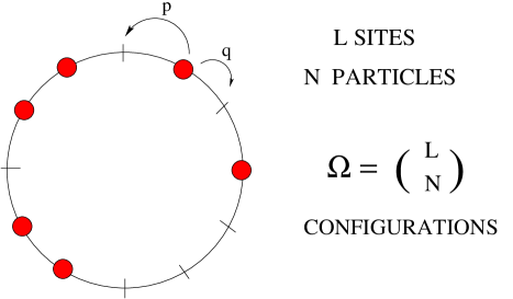
Figure 1: The Asymmetric exclusion process on a periodic ring.

We call $P_{t}(\mathcal{C})$ the probability of configuration $\mathcal{C}$ at time $t$. As the exclusion process is a continuous-time Markov process, the time evolution of $P_{t}(\mathcal{C})$ is determined by the master equation

$$\frac{d}{dt}P_{t}(\mathcal{C})=\sum_{\mathcal{C}^{\prime}}M(\mathcal{C},\mathcal{C}^{\prime})P_{t}(\mathcal{C}^{\prime})=\sum_{\mathcal{C}^{\prime}}\Big{(}M_{0}(\mathcal{C},\mathcal{C}^{\prime})+M_{1}(\mathcal{C},\mathcal{C}^{\prime})+M_{-1}(\mathcal{C},\mathcal{C}^{\prime})\Big{)}P_{t}(\mathcal{C}^{\prime})\,.$$ (1)

The Markov matrix $M$ encodes the dynamics of the exclusion process: the non-diagonal element $M_{1}(\mathcal{C},\mathcal{C}^{\prime})$ represents the transition rate from configuration $\mathcal{C}^{\prime}$ to $\mathcal{C}$ where a particle hops in the forward (i.e., anti-clockwise) direction, the non-diagonal element $M_{-1}(\mathcal{C},\mathcal{C}^{\prime})$ represents the transition rate from configuration $\mathcal{C}^{\prime}$ to $\mathcal{C}$ where a particle hops in the backward (i.e., clockwise) direction. The diagonal term $M_{0}(\mathcal{C},\mathcal{C})=-\sum_{\mathcal{C}^{\prime}\neq\mathcal{C}}\left(M_{1}(\mathcal{C}^{\prime},\mathcal{C})+M_{-1}(\mathcal{C}^{\prime},\mathcal{C})\right)$ represents the exit rate from the configuration $\mathcal{C}$.

The matrix $M$ is a real non-symmetric matrix and, therefore, its eigenvalues (and eigenvectors) are either real numbers or complex conjugate pairs. A right eigenvector $P$ is associated with the eigenvalue $E$ of $M$ if

$$MP=EP\,.$$ (2)

On a ring the total number $N$ of particles is conserved. For a given value of $N$, the dynamics is ergodic (i.e., $M$ is irreducible and aperiodic). The Perron-Frobenius theorem implies that 0 is a non-degenerate eigenvalue and that all other eigenvalues have a strictly negative real part; the relaxation time of the corresponding eigenmode is $\tau=-1/\mathrm{Re}(E)$. The right eigenvector corresponding to the eigenvalue $E=0$ is the stationary state : for the ASEP on a ring the steady state is uniform and the stationary probability of any configuration $\mathcal{C}$ is given by $P(\mathcal{C})=N!(L-N)!/L!$.

Remark : A configuration can also be characterized by the positions of the $N$ particles on the ring, $(x_{1},x_{2},\dots,x_{N})$ with $1\leq x_{1}<x_{2}<\dots<x_{N}\leq L$. With this representation, the eigenvalue equation (2) becomes

$$EP(x_{1},\dots,x_{N})=$$

$$\sum_{i}p\left[P(x_{1},\dots,x_{i-1},\ x_{i}-1,\ x_{i+1},\dots,x_{N})-P(x_{1},\dots,x_{n})\right]+$$

$$\sum_{j}q\left[P(x_{1},\dots,x_{j-1},\ x_{j}+1,\ x_{j+1},\dots,x_{N})-P(x_{1},\dots,x_{N})\right]\,,$$ (3)

where the sum runs over the indexes $i$ such that $x_{i-1}<x_{i}-1$ and over the indexes $j$ such that $x_{j}+1<x_{j+1}\,;$ these inequalities ensure that the corresponding jumps are allowed.

The knowledge of the spectrum of the matrix $M$ and of the associated eigenvectors provides a full description of the dynamics of the model. Such a spectral analysis is very similar to that carried out in Quantum Mechanics. One should however keep in mind that in the present case the evolution operator is non-hermitian : its eigenvalues are complex numbers and the associated eigenvectors do not form an orthogonal basis in the configuration space. Moreover, because $M$ is not symmetric, its left eigenvectors are different from the right eigenvectors.

II.2 Natural symmetries of ASEP on a periodic ring

Before diagonalizing the Markov matrix $M$ by Bethe Ansatz, we present some invariance properties of the ASEP, that can be described using elementary methods. The exclusion process on a ring displays symmetry properties under translation, right-left reflection, and particle/hole exchange (the last two symmetries play a role analogous to parity and charge conjugaison in quantum mechanics). These symmetries reveal some intrinsic formal properties of the Markov matrix, and are very useful to reduce the computation time when numerical diagonalization is performed. Finally, these natural symmetries will allow us to define some conserved quantities (analogous to quantum numbers) and to predict degeneracies in the spectrum.

II.2.1 Translation invariance

The translation operator $T$ shifts simultaneously all the particles one site forward:

$$T(\tau_{1},\tau_{2},\ldots,\tau_{L})=(\tau_{L},\tau_{1},\tau_{2},\ldots,\tau_{L-1})\,.$$ (4)

Because of the periodicity we have $T^{L}=1$. Thus, the eigenvalues (or impulsions) $k$ of $T$ are simply the $L$-th roots of unity:

$$k=e^{2i\pi m/L}\ \ \,\hbox{ for }m=0,\ldots,L-1\,.$$ (5)

We denote by ${\bf T}(k)$ the eigenspace of $T$ corresponding to the impulsion $k$. The projection operator $\mathcal{T}_{k}$ over this eigenspace is given by

$$\mathcal{T}_{k}=\frac{1}{L}\sum_{r=0}^{L-1}k^{-r}T^{r}\,.$$ (6)

The complex conjugation transforms a $T$-eigenvector of eigenvalue $k$ into an eigenvector with eigenvalue $k^{*}=k^{-1}$, i.e., ${\bf T}(k^{*})=[{\bf T}(k)]^{*}$.

The ASEP on a periodic lattice is translation invariant, i.e.,

$$MT=TM\,.$$ (7)

The matrix $M$ and the translation operator $T$ can therefore be simultaneously diagonalized: $M$ leaves each eigenspace ${\bf T}(k)$ invariant. We denote by ${\bf Sp}(k)$ the set of the eigenvalues of $M$ restricted to ${\bf T}(k)$. Using complex conjugation we obtain the property

$${\bf Sp}(k^{*})=\left[{\bf Sp}(k)\right]^{*}\,.$$ (8)

II.2.2 Right-Left Reflection

The reflection operator $R$ interchanges the right and the left and is defined by

$$R(\tau_{1},\tau_{2},\ldots,\tau_{L})=(\tau_{L},\tau_{L-1},\ldots,\tau_{2},\tau_{1})\,.$$ (9)

We have $R^{2}=1$; the eigenvalues of $R$ are thus $r=\pm 1$. The reflection $R$ reverses the translations, i.e.,

$$RT=T^{-1}R\,,$$ (10)

and transforms a $T$-eigenvector of eigenvalue $k$ into an eigenvector of eigenvalue $k^{*}$. The operator $R$ does not commute with the Markov matrix because the asymmetric jump rates $(p\neq q)$ are not invariant under the exchange of right and left. Writing explicitly the dependence of $M$ on the jump rates, we have

$$RM_{(p,q)}R^{-1}=M_{(q,p)}\,.$$ (11)

Thus, in general the reflection is not a symmetry of the ASEP (only the symmetric exclusion process is invariant under reflection).

II.2.3 Charge conjugation

The charge conjugation operator $C$ exchanges particles and holes in the system, i.e., a configuration with $N$ particles is mapped into a configuration with $L-N$ particles:

$$C(\tau_{1},\tau_{2},\ldots,\tau_{L})=(1-\tau_{1},1-\tau_{2},\ldots,1-\tau_{L})\,.$$ (12)

The operator $C$ satisfies the relations:

$$C^{2}=1,\,\,\,\,\,CT=TC,\,\,\,\,\,CR=RC\,.$$ (13)

By charge conjugation, particles jumping forward are mapped into holes jumping forward. But holes jumping forward are equivalent to particles jumping backward. Writing explicitly the dependence of $M$ on the number $N$ of particles and on the jump rates, we thus have

$$CM_{(N,p,q)}C^{-1}=M_{(L-N,q,p)}\,.$$ (14)

We notice that the number of particles is conserved by $C$ only at half filling ($L=2N$). Thus, the charge conjugation is not a symmetry of the ASEP except for the symmetric $(p=q)$ exclusion process at half filling.

II.2.4 CR symmetry

Using equations (11) and (14) to combine the charge conjugation $C$ with the reflection $R$, we obtain

$$(CR)M_{(N,p,q)}(CR)^{-1}=M_{(L-N,p,q)}\,.$$ (15)

Thus, for a given $L$, the $CR$ operator maps the ASEP with $N$ particles into the ASEP with the same jumping rates but with $L-N$ particles. This implies that the spectrum of $M$ for $N$ particles is identical with the spectrum for $L-N$ particles (because $CR$ transforms eigenvectors of $M_{(N,p,q)}$ into eigenvectors of $M_{(L-N,p,q)}$).

For the ASEP model at half filling, i.e., $L=2N$, the $CR$ operator constitutes an exact symmetry :

$$(CR)\,M=M\,(CR)\,.$$ (16)

The ASEP at half filling is therefore invariant under each of the two symmetries, translation $T$ and $CR$. Note that they do not commute with each other; we rather obtain from equations (10) and (13)

$$(CR)T=T^{-1}(CR)\,.$$ (17)

Hence, the $CR$ transformation maps the subspace ${\bf T}(k)$ into ${\bf T}(k^{*})$ and thus ${\bf Sp}(k)={\bf Sp}(k^{*})\,.$ For $k\neq\pm 1$, the subspaces ${\bf T}(k)$ and ${\bf T}(k^{*})$ are distinct and the corresponding eigenvalues of $M$ are doubly degenerate. For $k=\pm 1$, the $CR$ transformation leaves ${\bf T}(k)$ invariant. Thus, the natural symmetries do not predict any degeneracies in the sets ${\bf Sp}(\pm 1)$. However, each of the subspaces ${\bf T}(\pm 1)$ is split into two smaller subspaces which are invariant under $CR$ and on which $CR=\pm 1$. For the ASEP at half filling, we find from Equation (8) that the set ${\bf Sp}(k)$ is self-conjugate, for all $k$, and degenerate with ${\bf Sp}(k^{*})$

$${\bf Sp}(k)=\left[{\bf Sp}(k)\right]^{*}={\bf Sp}(k^{*})\,.$$ (18)

This means that ${\bf Sp}(k)$, for all $k$, is made only of real numbers or of complex conjugate pairs.

III Algebraic Bethe Ansatz for the Exclusion Process

III.1 The algebra of local update operators

The space of all possible configurations ${C}$ is a $2^{L}$ dimensional vector space that we shall denote by $\mathcal{S}$. Each site $i$ is either occupied or empty : we shall represent its state by the local basis $(|1\rangle_{i},|0\rangle_{i})$ of the two dimensional space ${\mathbb{C}}^{2}_{i}$. The total configuration space $\mathcal{S}$ is thus given by

$$\mathcal{S}={\mathbb{C}}^{2}_{1}\otimes{\mathbb{C}}^{2}_{2}\otimes\ldots\otimes{\mathbb{C}}^{2}_{L}\,,$$ (19)

The natural basis of the configuration space $\mathcal{S}$ is the tensor product $(|1\rangle_{1},|0\rangle)_{1}\otimes\ldots\otimes(|1\rangle_{L},|0\rangle)_{L}$. On a periodic lattice, the number $N$ of particles is conserved by the dynamics. The total number of configurations for $N$ particles on a ring with $L$ sites is given by $\mathcal{N}=L!/[N!(L-N)!]$. The allowed configurations of the system span a subspace of $\mathcal{S}$ of dimension $\mathcal{N}$. The Markov matrix can be expressed as a sum of local operators that update the bond $(i,i+1)$ :

$$M=\sum_{i=1}^{L}M_{i,i+1}\,,.$$ (20)

The update operator $M_{i,i+1}$ is given by

$$M_{i,i+1}={\bf 1}_{1}\otimes{\bf 1}_{2}\ldots{\bf 1}_{i-1}\otimes\left(\begin{array}[]{cccc}0&0&0&0\\ 0&-p&q&0\\ 0&p&-q&0\\ 0&0&0&0\end{array}\hskip 14.45377pt\right)\otimes{\bf 1}_{i+2}\ldots{\bf 1}_{L}\,,$$ (21)

where ${\bf 1}_{j}$ is the $2\times 2$ identity matrix acting on the site number $j$. We emphasize that $M_{i,i+1}$ is a $2^{L}\times 2^{L}$ matrix that acts trivially on all sites different from $i$ and $i+1$ and updates the bond $(i,i+1)$ according to the local dynamical rules of the exclusion process. We also define the local permutation operator $P_{i,i+1}$

$$P_{i,i+1}={\bf 1}_{1}\otimes{\bf 1}_{2}\ldots{\bf 1}_{i-1}\otimes\left(\begin{array}[]{cccc}1&0&0&0\\ 0&0&1&0\\ 0&1&0&0\\ 0&0&0&1\end{array}\hskip 14.45377pt\right)\otimes{\bf 1}_{i+2}\ldots{\bf 1}_{L}\,.$$ (22)

The local update operators satisfy the following relations:

$$P_{i,i+1}M_{i,i+1} = -M_{i,i+1}\,$$ (23)

$$M_{i,i+1}^{2} = -M_{i,i+1}\,$$ (24)

$$M_{i,i+1}\,M_{i+1,i+2}\,M_{i,i+1} = pq\,M_{i,i+1}\,$$ (25)

$$M_{i,i+1}\,M_{i-1,i}\,M_{i,i+1} = pq\,M_{i,i+1}\,$$ (26)

$$\,[M_{i,i+1},M_{j,j+1}] = 0\,\,\,\hbox{ for }|i-j|\geq 2\,.$$ (27)

These identities define a Temperley-Lieb algebra : this property of reaction-diffusion processes was emphasized by Alcaraz et al. (1994) and plays a key-role in the integrability of the ASEP.

III.2 The ASEP as a non-Hermitian spin chain

The dynamics of the ASEP is entirely encoded in its Markov matrix $M$ that governs the time evolution of the probability measure on the configuration space. We now show that the local operator $M_{i,i+1}$ that updates the bond $(i,i+1)$ located in the bulk of the system can be expressed with the help of the Pauli matrices. We recall that Pauli matrices are given by

$$S^{x}=\left(\begin{array}[]{cc}0&1\\ 1&0\end{array}\right)\,,\,\,\,\,\,\,\,\,\,\,S^{y}=\left(\begin{array}[]{cc}0&-i\\ i&0\end{array}\right)\,,\,\,\,\,\,\,\,\,\,\,S^{z}=\left(\begin{array}[]{cc}1&0\\ 0&-1\end{array}\right)\,\,\,\,\,.$$ (28)

We also need the following operators

$$S^{+}=\frac{S^{x}+iS^{y}}{2}=\left(\begin{array}[]{cc}0&1\\ 0&0\end{array}\right)\,,\,\,\,\,\,S^{-}=\frac{S^{x}-iS^{y}}{2}=\left(\begin{array}[]{cc}0&0\\ 1&0\end{array}\right)\,\,\,\,\,.$$ (29)

After identifying the spin-$\frac{1}{2}$ basis $(|\uparrow\rangle,|\downarrow\rangle)$ of ${\mathbb{C}}^{2}$ with the local basis $(|1\rangle_{i},|0\rangle_{i})$ of the two-dimensional space ${\mathbb{C}}^{2}_{i}$ associated with the site $i$, we define an action of the Pauli matrices on the ASEP configuration space $\mathcal{S}$ as follows :

$$S^{a}_{i}={\bf 1}_{1}\otimes\ldots\otimes{\bf 1}_{i-1}\otimes S^{a}\otimes{\bf 1}_{i+1}\otimes\ldots{\bf 1}_{L}\,\,\,\hbox{ with }\,\,\,a=x,y,z,+,-\,.\\$$ (30)

We observe that the local update operator $M_{i,i+1}$ can be written as

$$M_{i,i+1}=pS^{-}_{i}S^{+}_{i+1}+qS^{+}_{i}S^{-}_{i+1}+\frac{1}{4}S^{z}_{i}S^{z}_{i+1}-\frac{p-q}{4}(S^{z}_{i}-S^{z}_{i+1})-\frac{1}{4}\,,$$ (31)

where ${\bf 1}$ represents the identity operator. The Markov matrix of the ASEP on the periodic lattice of size $L$ is thus given by

$$M=\sum_{i=1}^{L}\left(pS^{-}_{i}S^{+}_{i+1}+qS^{+}_{i}S^{-}_{i+1}+\frac{1}{4}S^{z}_{i}S^{z}_{i+1}\right)-\frac{L}{4}\,,$$ (32)

(we recall that the site $L+1$ is the same as the site number 1). The Markov matrix is therefore expressed as a spin chain on the periodic lattice. This spin chain is non-Hermitian when $p\neq q$. For $p=q=1/2$, the Markov matrix $M$ is identical with the antiferromagnetic Heisenberg XXX spin chain which was exactly solved by Hans Bethe (1931). More generally, a similarity transformation allows us to map exactly the Markov matrix $M$ on an antiferromagnetic XXY quantum spin chain with hermiticity breaking boundary terms. Following Essler and Rittenberg (1996), we consider the operators

$$U_{i}={\bf 1}_{1}\otimes\ldots\otimes{\bf 1}_{i-1}\otimes\left(\begin{array}[]{cc}1&0\\ 0&\alpha^{i-1}\end{array}\right)\otimes{\bf 1}_{i+1}\otimes\ldots{\bf 1}_{L}\,,$$ (33)

where we have defined

$$\alpha=\sqrt{\frac{p}{q}}\,.$$ (34)

The operator $H$ defined as

$$H=(\alpha+\alpha^{-1})\left(\prod_{i=1}^{L}U_{i}\right)\left(M+\frac{L}{4}{\bf 1}\right)\left(\prod_{i=1}^{L}U_{i}\right)^{-1}\,,$$ (35)

is then given by

$$H=\frac{1}{2}\sum_{i=1}^{L-1}\left(S^{x}_{i}S^{x}_{i+1}+S^{y}_{i}S^{y}_{i+1}+\frac{\alpha+\alpha^{-1}}{2}S^{z}_{i}S^{z}_{i+1}\right)+\alpha^{L}S^{-}_{L}S^{+}_{1}+\alpha^{-L}S^{+}_{L}S^{-}_{1}+\frac{\alpha+\alpha^{-1}}{4}S^{z}_{L}S^{z}_{1}\,.$$ (36)

In this representation, we can formally rewrite $H$ as the XXY spin chain on a periodic lattice with the following twisted boundary conditions

$$S^{+}_{L+1} = \alpha^{L}S^{+}_{1}$$

$$S^{-}_{L+1} = \alpha^{-L}S^{-}_{1}$$

$$S^{z}_{L+1} = S^{z}_{1}\,.$$ (37)

III.3 The Yang-Baxter equation

We shall now derive the Yang-Baxter equation which will allow us to define in the subsection III.4 a one-parameter family of commuting operators that contains the Markov matrix $M$. Such a family of commuting operators ensures the existence of a sufficient number of conserved quantities that fully label the states of the ASEP. This property is the key to the integrability of the ASEP.

Let us consider two auxiliary sites labeled as $a$ and $b$, each of them having two possible states $(|1\rangle_{a},|0\rangle_{a})$ and $(|1\rangle_{b},|0\rangle_{b})$ respectively. The four possible states of $a$ and $b$ span a four dimensional complex vector space denoted as ${\mathcal{A}}\otimes{\mathcal{B}}$. For any given value of the complex number $\lambda$ (called the spectral parameter), we define an operator ${\mathcal{L}}_{ab}(\lambda)$ which acts on this tensor space as follows

$${\mathcal{L}}_{ab}(\lambda)=P_{ab}\left(1+\lambda M_{ab}\right)\,,$$ (38)

where $M_{ab}$ and $P_{ab}$ represent the jump and the permutation operators between $a$ and $b$ as defined in equations (21) and (22) respectively. We emphasize that the auxiliary sites $a$ and $b$ should not be viewed as neighbouring sites on a given lattice but rather as an ‘abstract’ pair of sites related by non-local jump and exchange operators $M_{ab}$ and $P_{ab}$. We now consider three auxiliary sites $a$, $b$ and $c$, and prove the Yang-Baxter relation :

$${\mathcal{L}}_{ab}(\nu){\mathcal{L}}_{cb}(\lambda){\mathcal{L}}_{ca}(\mu)={\mathcal{L}}_{ca}(\mu){\mathcal{L}}_{cb}(\lambda){\mathcal{L}}_{ab}(\nu)\,\,\,\hbox{ for }\,\,\,\nu=\frac{\lambda-\mu}{1-\mu+pq\lambda\mu}\,.$$ (39)

We shall need the fact that the jump and permutation operators between the auxiliary sites satisfy the following relations analogous to (23–27). For example, we have

$$P_{c,a}M_{a,b} = M_{c,b}P_{c,a}\,$$ (40)

$$M_{a,b}^{2} = -M_{a,b}\,$$ (41)

$$M_{c,a}\,M_{a,b}\,M_{c,a} = pqM_{c,a}\,\,$$ (42)

$$M_{a,b}\,M_{c,a}\,M_{a,b} = pqM_{a,b}\,\,.$$ (43)

In order to derive the Yang-Baxter equation, we first remark that

$${\mathcal{L}}_{ab}(\nu){\mathcal{L}}_{cb}(\lambda){\mathcal{L}}_{ca}(\mu) = P_{ab}\left(1+\nu M_{ab}\right)P_{cb}\left(1+\lambda M_{cb}\right)P_{ca}\left(1+\mu M_{ca}\right)$$ (44)

$$= P_{ab}\left(1+\nu M_{ab}\right)P_{cb}P_{ca}\left(1+\lambda M_{ab}\right)\left(1+\mu M_{ca}\right)$$

$$= P_{ab}P_{cb}P_{ca}\left(1+\nu M_{ca}\right)\left(1+\lambda M_{ab}\right)\left(1+\mu M_{ca}\right)\,.$$

Similarly, we have

$${\mathcal{L}}_{ca}(\mu){\mathcal{L}}_{cb}(\lambda){\mathcal{L}}_{ab}(\nu)=P_{ca}P_{cb}P_{ab}\left(1+\mu M_{ab}\right)\left(1+\lambda M_{ca}\right)\left(1+\nu M_{ab}\right)\,.$$ (45)

Now, with the help of the Temperley-Lieb algebra, equations (23–27), we obtain

$$\left(1+\nu M_{ca}\right)\left(1+\lambda M_{ab}\right)\left(1+\mu M_{ca}\right)$$ (46)

$$= 1+(\mu+\nu)M_{ca}+\lambda M_{ab}+\mu\nu M_{ca}^{2}+\lambda\mu M_{ab}M_{ca}+\lambda\nu M_{ca}M_{ab}+\lambda\mu\nu M_{ca}M_{ab}M_{ca}$$

$$= 1+(\mu+\nu-\mu\nu+pq\lambda\mu\nu)M_{ca}+\lambda M_{ab}+\lambda\mu M_{ab}M_{ca}+\lambda\nu M_{ca}M_{ab}\,.$$

Similarly we have

$$\left(1+\mu M_{ab}\right)\left(1+\lambda M_{ca}\right)\left(1+\nu M_{ab}\right)$$ (47)

$$= 1+(\mu+\nu-\mu\nu+pq\lambda\mu\nu)M_{ab}+\lambda M_{ca}+\lambda\mu M_{ab}M_{ca}+\lambda\nu M_{ca}M_{ab}\,.$$

Using the fact that $P_{ab}P_{cb}P_{ca}=P_{ca}P_{cb}P_{ab}$ we complete the proof of equation (39).

III.4 The Transfer Matrix

We are now ready to apply the Algebraic Bethe Ansatz to the ASEP (for introduction to this subject, see Faddeev 1984, de Vega 1989, and Nepomechie 1999). We introduce an auxiliary site (denoted as site 0) which can be in two states $|1\rangle_{0}$ or $|0\rangle_{0}$. These two states span a two dimensional vector space, ${\mathcal{A}}$, the auxiliary space. We define, as in equation (38), a local transfer operator ${\mathcal{L}}_{i0}(\lambda)$ between the site $i$ of the ASEP ring and the auxiliary site 0. This operator, that we shall denote as ${\mathcal{L}}_{i}(\lambda)$, can be represented as a $2\times 2$ operator on the vector space ${\mathcal{A}}$,

$${\mathcal{L}}_{i}(\lambda)=\left(\begin{array}[]{cc}a(\lambda)&b(\lambda)\\ c(\lambda)&d(\lambda)\end{array}\right)\,,$$ (48)

where the matrix elements $a(\lambda),b(\lambda),c(\lambda)$ and $d(\lambda)$ are themselves $2^{L}\times 2^{L}$ operators that act on the configuration space ${\mathcal{S}}$. These operators act trivially on all sites different from $i$ and are given by

$$a(\lambda) = {\bf 1}_{1}\otimes\ldots{\bf 1}_{i-1}\otimes\left(\begin{array}[]{cc}1&0\\ 0&q\lambda\end{array}\right)\otimes{\bf 1}_{i+1}\ldots{\bf 1}_{L}\,,$$ (51)

$$b(\lambda) = {\bf 1}_{1}\otimes\ldots{\bf 1}_{i-1}\otimes\left(\begin{array}[]{cc}0&0\\ 1-p\lambda&0\end{array}\right)\otimes{\bf 1}_{i+1}\ldots{\bf 1}_{L}\,,$$ (54)

$$c(\lambda) = {\bf 1}_{1}\otimes\ldots{\bf 1}_{i-1}\otimes\left(\begin{array}[]{cc}0&1-q\lambda\\ 0&0\end{array}\right)\otimes{\bf 1}_{i+1}\ldots{\bf 1}_{L}\,,$$ (57)

$$d(\lambda) = {\bf 1}_{1}\otimes\ldots{\bf 1}_{i-1}\otimes\left(\begin{array}[]{cc}p\lambda&0\\ 0&1\end{array}\right)\otimes{\bf 1}_{i+1}\ldots{\bf 1}_{L}\,.$$ (60)

We now consider the operator

$${\mathcal{R}}(\nu)=1+\nu M_{a^{\prime},a}\,,$$ (61)

that acts on ${\mathcal{A}}\otimes{\mathcal{A}}^{\prime}$ where the auxiliary spaces ${\mathcal{A}}$ and ${\mathcal{A}}^{\prime}$ are the configuration spaces of the auxiliary sites $a$ and $a^{\prime}$. In the basis $\left(|1_{a},1_{a^{\prime}}\rangle,|1_{a},0_{a^{\prime}}\rangle,|0_{a},1_{a^{\prime}}\rangle,|0_{a},0_{a^{\prime}}\rangle\right)$ of ${\mathcal{A}}\otimes{\mathcal{A}}^{\prime}$, the operator ${\mathcal{R}}(\nu)$ is represented by a $4\times 4$ scalar matrix :

$${\mathcal{R}}(\nu)=\left(\begin{array}[]{cccc}1&0&0&0\\ 0&1-q\nu&p\nu&0\\ 0&q\nu&1-p\nu&0\\ 0&0&0&1\end{array}\right)\,.$$ (62)

Using equation (39), we find that the operators ${\mathcal{L}}_{i}(\lambda)$ satisfy the Yang-Baxter equation :

$${\mathcal{R}}(\nu)\big{[}{\mathcal{L}}_{i}(\lambda)\otimes{\mathcal{L}^{\prime}}_{i}(\mu)\big{]}=\big{[}{\mathcal{L}}_{i}(\mu)\otimes{\mathcal{L}^{\prime}}_{i}(\lambda)\big{]}{\mathcal{R}}(\nu)\,\,\,{\rm with}\,\,\,\nu=\frac{\lambda-\mu}{1-\mu+pq\lambda\mu}\,,$$ (63)

where ${\mathcal{L}}_{i}$ and ${\mathcal{L}^{\prime}}_{i}$ are interpreted as $2\times 2$ matrices acting, respectively, on ${\mathcal{A}}$ and ${\mathcal{A}^{\prime}}$ with elements that are themselves operators on ${\mathcal{S}}$. Their tensor product is thus a $4\times 4$ matrix, acting on ${\mathcal{A}}\otimes{\mathcal{A}^{\prime}}$ with matrix elements that are operators on ${\mathcal{S}}$.

The monodromy matrix is defined as

$$T(\lambda)={\mathcal{L}}_{1}(\lambda){\mathcal{L}}_{2}(\lambda)\ldots{\mathcal{L}}_{L}(\lambda)\,,$$ (64)

where the product of the ${\mathcal{L}}_{i}$’s has to be understood as a product of $2\times 2$ matrices acting on ${\mathcal{A}}$ with non-commutative elements. The monodromy matrix $T(\lambda)$ can thus be written as

$$T(\lambda)=\left(\begin{array}[]{cc}A(\lambda)&B(\lambda)\\ C(\lambda)&D(\lambda)\end{array}\right)\,,$$ (65)

where $A,B,C$ and $D$ are operators on the configuration space ${\mathcal{S}}$. By applying equation (63) to all the lattice sites $i$, we find that the monodromy matrix satisfies a similar relation

$${\mathcal{R}}(\nu)\big{[}T(\lambda)\otimes T(\mu)\big{]}=\big{[}T(\mu)\otimes T(\lambda)\big{]}{\mathcal{R}}(\nu)\,\,\,{\rm with}\,\,\,\nu=\frac{\lambda-\mu}{1-\mu+pq\lambda\mu}\,,$$ (66)

Taking the trace of the monodromy matrix over the auxiliary space $\mathcal{A}$, we obtain a one-parameter family of transfer matrices acting on ${\mathcal{S}}$

$$t(\lambda)={\rm Tr}_{\mathcal{A}}(T(\lambda))=A(\lambda)+D(\lambda)\,.$$ (67)

By taking the trace of equation (66) over ${\mathcal{A}}\otimes{\mathcal{A}^{\prime}}$ and using the fact that ${\mathcal{R}}(\nu)$ is generically an invertible matrix, we deduce that the operators $t(\lambda)$ form a family of commuting operators (see e.g., Nepomechie, 1999). In particular, this family contains the translation operator ${T}=t(0)$ (that shifts all the particles simultaneously one site forward) and the Markov matrix $M=t^{\prime}(0)/t(0)$.

The equation (66), when written explicitly, leads to 16 quadratic relations between the operators $A(\lambda)$, $B(\lambda)$, $C(\lambda)$, $D(\lambda)$ and the operators $A(\mu),B(\mu),C(\mu),D(\mu)$. In particular, we have

$$C(\lambda)C(\mu) = C(\mu)C(\lambda)\,,$$ (68)

$$A(\lambda)C(\mu) = (1-q\nu)A(\mu)C(\lambda)+p\nu C(\mu)A(\lambda)\,,$$ (69)

$$D(\lambda)C(\mu) = p\nu C(\mu)D(\lambda)+(1-p\nu)D(\mu)C(\lambda)\,.$$ (70)

These relations are used in the next subsection to construct the eigenvectors of the family of transfer matrices $t(\lambda)$.

III.5 The Bethe equations

Using Algebraic Bethe Ansatz, the common eigenvectors of this family are explicitly constructed by actions of the $C$ operators on the reference state $\Omega$, defined as

$$\Omega=|0_{1}0_{2}\ldots 0_{L}\rangle\,.$$ (71)

The state $\Omega$ corresponds to a configuration where all the sites are empty. The operators $A(\lambda)$ and $D(\lambda)$ have a simple action on $\Omega$, namely

$$A\left(\frac{\lambda}{q}\right)\,\Omega=\lambda^{L}\,\Omega\,\,\,\,\hbox{ and }\,\,\,\,D\left(\frac{\lambda}{q}\right)\,\Omega=\,\Omega\,.$$ (72)

Now, for any $N\leq L$, we define the vector

$$|z_{1},z_{2}\ldots z_{N}\rangle=C\left(\frac{z_{N}}{q}\right)\ldots C\left(\frac{z_{2}}{q}\right)C\left(\frac{z_{1}}{q}\right)\,\Omega\,,$$ (73)

where $z_{1},z_{2}\ldots z_{N}$ are complex numbers. Each operator $C$ creates a particle in the system, and the state $|z_{1},z_{2}\ldots z_{N}\rangle$ is a linear combination of configurations with exactly $N$ particles. This vector is an eigenvector of the operator $t(\lambda/q)$ (for all values of $\lambda$) and in particular of the Markov matrix M, provided the pseudo-momenta $z_{1}$, $z_{2}$, $\ldots$, $z_{N}$ satisfy the Bethe equations (Gwa and Spohn 1992) :

$$z_{l}^{L}=(-1)^{N-1}\prod_{i=1}^{N}\frac{pz_{l}z_{i}-z_{l}+q}{pz_{l}z_{i}-z_{i}+q}\,\,\,{\rm for}\,\,\,\,l=1\ldots N\,.$$ (74)

These equations are derived by considering the action of the operators $t(\lambda/q)$ on $|z_{1},z_{2}\ldots z_{N}\rangle$ :

$$t\left(\frac{\lambda}{q}\right)\,|z_{1},z_{2}\ldots z_{N}\rangle=A\left(\frac{\lambda}{q}\right)\,C\left(\frac{z_{N}}{q}\right)\ldots C\left(\frac{z_{2}}{q}\right)C\left(\frac{z_{1}}{q}\right)\,\Omega+D\left(\frac{\lambda}{q}\right)\,C\left(\frac{z_{N}}{q}\right)\ldots C\left(\frac{z_{2}}{q}\right)C\left(\frac{z_{1}}{q}\right)\,\Omega\,.$$ (75)

Applying repeatedly equations (69) and (70) to the first term and to the second term on the r.h.s. of this equation, respectively, we obtain a linear combination of $|z_{1},z_{2}\ldots z_{N}\rangle$ and of $N$ vectors $|z_{1},\ldots z_{i-1},\lambda,z_{i+1}z_{N}\rangle$ for $i=1,\ldots,N$. If we want $|z_{1},z_{2}\ldots z_{N}\rangle$ to be an eigenvector of $t(\lambda/q)$, the coefficients of these $N$ vectors must vanish . The vanishing conditions for the coefficients of the unwanted terms provide a set of $N$ relations that must be satisfied by the complex numbers $z_{1},z_{2}\ldots z_{N}$. These relations, when written explicitly, are precisely the Bethe equations (74).

The corresponding eigenvalue of $t(\lambda/q)$ is given by

$$\mathcal{E}(\lambda;z_{1},z_{2}\ldots z_{N})=\prod_{i=1}^{N}\frac{p\lambda z_{i}-\lambda+q}{z_{i}-\lambda}+\lambda^{L}\prod_{i=1}^{N}\frac{p\lambda z_{i}-z_{i}+q}{\lambda-z_{i}}\,.$$ (76)

Using the Bethe equations (74), we find that $\mathcal{E}(\lambda)$ is a polynomial in $\lambda$ of degree $L-N$. The eigenvalue of the Markov matrix is given by

$$E(z_{1},z_{2}\ldots z_{N})=p\sum_{i=1}^{N}z_{i}+q\sum_{i=1}^{N}\frac{1}{z_{i}}-N\,.$$ (77)

The Bethe equations (74) for the ASEP were first derived and analyzed by Gwa and Spohn (1992), who used the coordinate Bethe Ansatz, a method more elementary and quicker than the one presented here. We have chosen to describe here the more sophisticated Algebraic Bethe Ansatz technique, because, in our opinion, the ASEP provides the simplest pedagogical example of this method. Besides, the Algebraic Bethe Ansatz becomes unavoidable to study exclusion processes with different classes of particles and systems with open boundaries (de Gier and Essler 2005). Finally, the Algebraic Bethe Ansatz allows to construct a Matrix Product Ansatz involving quadratic algebras and to draw a rigorous relation between the two complementary approaches used to analyze the ASEP (Golinelli and Mallick 2006).

IV Analysis of the Bethe equations of the TASEP

In the limit of a totally asymmetric exclusion process the Bethe equations become particularly simple and can be analyzed thoroughly. In this section we present some exact results that are valid for the TASEP. Substituting $p=0$ and $q=1$ in the Bethe equations (74), we obtain

$$z_{i}^{L}=(-1)^{N-1}\prod_{j=1}^{N}\frac{1-z_{i}}{1-z_{j}}\,\,\,{\rm for}\,\,\,\,i=1\ldots N\,.$$ (78)

In terms of the variables $Z_{i}=2/z_{i}-1$, these equations become (Gwa and Spohn 1992)

$$(1-Z_{i})^{N}\ (1+Z_{i})^{L-N}=-2^{L}\prod_{j=1}^{N}\frac{Z_{j}-1}{Z_{j}+1}\ \ \ \hbox{for}\ \ \ i=1,\dots,N\,.$$ (79)

We note that the right-hand side of these equations is independent of the index $i$: this property is true only for the TASEP where the Bethe equations decouple and can be reduced to an effective one-variable equation. The corresponding eigenvalue $E$ of the Markov matrix $M$ is given by

$$2E=-N+\sum_{j=1}^{N}Z_{j}\,.$$ (80)

For the TASEP, it is possible to show that the associated Bethe eigenvector $P_{E}$ is a determinant (Golinelli and Mallick 2005b)

$$P_{E}(x_{1},\dots,x_{N})=\det(R)\,,$$ (81)

where $R$ is a $N\times N$ matrix with elements

$$R(i,j)=\frac{z_{i}^{x_{j}}}{(1-z_{i})^{j}}\ \ \mbox{for }1\leq i,j\leq N\,,$$ (82)

where $(z_{1},\dots,z_{N})$ are the roots of the Bethe equations (78). Similar formulae with determinants also appear in the expression of $P_{t}$ calculated for an arbitrary initial condition $P_{0}$ on an infinite open lattice (Schütz 1997, Sasamoto and Wadati 1998, Rákos and Schütz 2005) and on a periodic lattice (Priezzhev 2003).

IV.1 Layout of the solutions of the Bethe equations

The solutions of the Bethe equations (79) are the roots of the polynomial equation of degree $L$

$$(1-Z)^{N}(1+Z)^{L-N}=Y\,,$$ (83)

where $Y$ must be determined self-consistently by the r.h.s. of equation (79). In this subsection, we describe the geometrical layout of the roots of the polynomial (83) for an arbitrary value of the complex number $Y$.

The $L$ solutions $(Z_{1},\dots,Z_{L})$ of this equation display interesting geometric properties. We explain how to label these solutions so that each $Z_{k}(Y)$ becomes an analytic function of the parameter $Y$ in the complex plane with a branch cut along the real semi-axis $[0,+\infty)$.

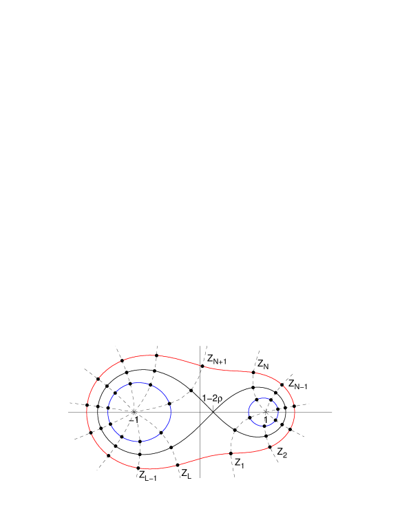
Figure 2: Labelling the roots of the Bethe equations. Here $L=15$, $N=6$, $\phi=\pi/2$ and $r/r_{c}=0.8,1,1.2$ (see text). The continuous curves are Cassini ovals. When $r$ is fixed and $\phi$ varies from 0 to $2\pi$, each $Z_{k}$ slips counterclockwise along a part of the Cassini oval. When $\phi$ is fixed and $r$ varies from $\infty$ to 0, each $Z_{k}$ travels along a dashed curve from $\infty$ to points +1 or -1.

A non-zero complex number $Y$ can be written in a unique way as

$$Y=r^{L}\,e^{i\phi}\ \ \mbox{with}\ \ 0\leq\phi<2\pi\ ,$$ (84)

$r$ being a positive real number. We emphasize that the argument has a branch cut along $[0,+\infty)$ : $\phi$ has a discontinuity of $2\pi$ when $Y$ crosses the positive real axis. For a given value of $r$, the complex numbers $Z_{k}$ belong to the generalised Cassini oval defined by

$$|Z-1|^{\rho}|Z+1|^{1-\rho}=r$$ (85)

where $\rho=N/L$ is the filling of the system. As shown in Fig. 2, the topology of the Cassini ovals depends on the value of $r$ with a critical value

$$r_{c}=2\rho^{\rho}(1-\rho)^{1-\rho}\,;$$ (86)

• for $r<r_{c}$, the curve consists of two disjoint ovals with $N$ solutions on the oval surrounding $+1$ and $L-N$ solutions on the oval surrounding $-1$.

• for $r=r_{c}$, the curve is a deformed Bernouilli lemniscate with a double point at $Z_{c}=1-2\rho$.

• for $r>r_{c}$, the curve is a single loop with $L$ solutions.

The Cassini ovals are symmetrical only if $\rho=1/2$.

In order to label the solutions, we start by considering the limit $r\to\infty$ for a given $\phi$. Equation (83) then becomes

$$Z^{L}\sim r^{L}\,\exp[i(\phi-N\pi)]\,.$$ (87)

The solutions $Z_{k}$ are given by

$$Z_{k}\sim r\,\exp\left[\frac{i}{L}[\phi-N\pi+2(k-1)\pi]\right]\ \ \mbox{with}\ \ k=1,\ldots,L\,.$$ (88)

In other words, the $Z_{k}$ are regularly distributed along a large circle of radius $r$ with

$$\frac{\phi-N\pi}{L}\leq\arg Z_{1}<\dots<\arg Z_{L}<\frac{\phi-N\pi}{L}+2\pi\,.$$ (89)

This labelling, obtained for large $r$, is extended by analytic continuation to all values of $r$, keeping $\phi$ fixed. The loci of the $Z_{k}$ are plotted in Fig. 2 (dashed curves): they are orthogonal to the Cassini ovals. A singularity appears along the branch $\phi=0$ because $Z_{1}$ and $Z_{N+1}$ collapse into each other at the double point $Z_{c}$ when $r=r_{c}$; we circumvent it by choosing $\phi=0^{+}$.

With this labelling, the solutions are ordered along the Cassini ovals. Moreover, when $r<r_{c}$, the solutions $(Z_{1},\dots,Z_{N})$ group together on the right oval and $(Z_{N+1},\dots,Z_{L})$ on the left oval.

IV.2 Procedure for solving the Bethe Equations

The special ‘one-body’ structure of the TASEP Bethe equations leads to the following self-consistent method for solving them. In the following sections, we shall show how this procedure can effectively be used to calculate the spectral gap of the model and to determine some arithmetical global properties of the spectrum.

• SOLVE, for any given value of $Y$, the polynomial equation $\,\,\,(1-Z_{i})^{N}(1+Z_{i})^{L-N}=Y\,.$ The $L$ roots $Z_{1}(Y)\,\ldots\,Z_{L}(Y)$ of this equation are located on a Cassini Oval

• CHOOSE $N$ roots $Z_{c(1)}(Y),\ldots\,Z_{c(N)}(Y)$ amongst the $L$ available roots, i.e., select a choice set $c:\{c(1),\ldots,c(N)\}\subset\{1,\ldots,L\}\,.$

• SOLVE the self-consistent equation ${A_{c}(Y)=Y}$ where

  $$A_{c}(Y)=-2^{L}\prod_{j=1}^{N}\frac{Z_{c(j)}(Y)-1}{Z_{c(j)}(Y)+1}\,.$$

  The self-consistent equation $A_{c}(Y)=Y$ is a fixed point equation. It is solved in practice by choosing iteratively a new $Y^{\prime}$ given by $Y^{\prime}=A_{c}(Y)$ and going back to the first step until convergence is reached.

• CALCULATE from the fixed point value of $Y$, the $Z_{c(j)}(Y)$’s and the energy corresponding to the choice set $c$ :

  $$2E_{c}(Y)=-N+\sum_{j=1}^{N}Z_{c(j)}(Y).$$

Consider the choice function $c_{0}(j)=j$ that selects the $N$ fugacities $Z_{i}$ with the largest real parts. The $A$-function and eigenvalue associated with this choice function are given by

$$A_{0}(Y) = -2^{L}\prod_{j=1}^{N}\frac{Z_{j}-1}{Z_{j}+1}\,,$$ (90)

$$2E_{0} = -N+\sum_{j=1}^{N}Z_{j}\,.$$ (91)

In (Golinelli and Mallick 2004a, 2005a), we derived the following exact combinatorial formulae for $A_{0}(Y)$ and $E_{0}(Y)$ for any finite values of $L$ and $N$ :

$$\log\frac{A_{0}(Y)}{Y} = \sum_{k=1}^{\infty}\left(\begin{array}[]{c}kL\\ kN\end{array}\right)\frac{Y^{k}}{k2^{kL}}\,,$$ (94)

$$E_{0}(Y) = -\sum_{k=1}^{\infty}\left(\begin{array}[]{c}kL-2\\ kN-1\end{array}\right)\frac{Y^{k}}{k2^{kL}}\,.$$ (97)

These expressions are derived as follows: when $Y\to 0$, the $N$ roots of the equation (83) with the largest real parts, i.e., $(Z_{1},\dots,Z_{N})$ converge to +1 (whereas the $L-N$ other roots go to -1). Consider a contour $\gamma$, positively oriented, that encircles +1 such that for $Y$ small enough $(Z_{1},\dots,Z_{N})$ are inside $\gamma$ whereas $(Z_{N+1},\dots,Z_{L})$ are outside $\gamma$. Let $h(Z)$ be a function, analytic in a domain that contains the contour $\gamma$; from the residue theorem, we deduce:

$$\sum_{j=1}^{N}h(Z_{j})=\frac{1}{2i\pi}\oint_{\gamma}\frac{(1-Z)^{N-1}(1+Z)^{L-N-1}(L-2N-LZ)}{(1-Z)^{N}(1+Z)^{L-N}-Y}h(Z){\rm d}Z\,.$$ (98)

The functions $\log\left({A_{0}(Y)}/{Y}\right)$ and $E_{0}(Y)$ are expressed as such contour integrals by choosing $h(Z)=\log(\frac{1+Z}{2})$ and $h(Z)=Z-1$, respectively. Equations (94) and (97) result from expanding for small values of $Y$ the denominator in equation (98), thanks to the formula $(A-Y)^{-1}=A^{-1}\sum_{k=0}^{\infty}Y^{k}/A^{k}$ valid for $|Y|<|A|$.

The expressions (94) and (97) are then analytically continued in ${\mathbb{C}}-[1,\infty)$. In the limit $L\to\infty$ and with $\rho$ fixed, we obtain from the Stirling formula

$$\ln\frac{A_{0}(Y)}{Y}\to\frac{1}{\sqrt{2\pi\rho(1-\rho)L}}\ \mathrm{Li}_{3/2}\left(\frac{Y}{r_{c}^{L}}\right)\,,$$ (99)

where $r_{c}$ was defined in equation (86) and the polylogarithm function $\mathrm{Li}_{s}$ of index $s$ is given by

$$\mathrm{Li}_{s}(z)=\frac{z}{\Gamma(s)}\ \int_{0}^{\infty}\frac{t^{s-1}\ dt}{e^{t}-z}=\sum_{k=1}^{\infty}\frac{z^{k}}{k^{s}}\,.$$ (100)

The function $\mathrm{Li}_{s}$ is defined by the first equality on the whole complex plane with a branch cut along the real semi-axis $[1,+\infty)$; the second equality is valid only for $|z|<1$. Similarly, when $L\to\infty$, $E_{0}(Y)$ can be expressed in terms of the polylogarithm function $\mathrm{Li}_{5/2}$.

From equation (94), we observe that the equation $A_{0}(Y)=Y$ has the solution $Y=0$ that yields $Z_{j}=1$ for $j\leq N$. This solution leads to $E_{0}=0$. The choice function $c_{0}(j)=j$ thus provides the ground state of the Markov matrix. This fact has been verified numerically for small size systems (Gwa and Spohn 1992, Golinelli and Mallick 2004a).

IV.3 Calculation of the Gap

The spectral gap, given by the first excited eigenvalue, corresponds to the choice $c_{1}(j)=j$ for $j=1,\ldots,N-1$ and $c_{1}(N)=N+1$ (Gwa and Spohn 1992). The associated self-consistency function and eigenvalue are given by

$$A_{1}(Y) = A_{0}(Y)\frac{Z_{N+1}-1}{Z_{N+1}+1}\ \frac{Z_{N}+1}{Z_{N}-1}\,,$$ (101)

$$2E_{1} = 2E_{0}+(Z_{N+1}-Z_{N})\,.$$ (102)

In the large $L$ limit, Bethe equations for the gap become at the leading order

$$\mathrm{Li}_{3/2}(-e^{u\pi})=2i\pi\left[(u+i)^{1/2}-(u-i)^{1/2}\right],\hbox{ where $u$ is defined as }\frac{Y}{r_{c}^{L}}=-{\rm e}^{u\pi}\,.$$ (103)

The solution of this equation is given by:

$$u=1.119\,068\,802\,804\,474\dots$$ (104)

This leads to the eigenvalue corresponding to the first excited state :

$$E_{1}=-2\sqrt{\rho(1-\rho)}\frac{6.509189337\ldots}{L^{3/2}}\pm\frac{2i\pi(2\rho-1)}{L}\,.$$ (105)

We observe that the first excited state consists in pair of conjugate complex numbers when $\rho$ is different from 1/2. The real part of $E_{1}$ describes the relaxation towards the stationary state. The corresponding relaxation time scales as the size $L$ of the system raised to the power 3/2; the dynamical exponent $z$ of the ASEP is thus given by $z=3/2$. This value agrees with the dynamical exponent of the one-dimensional Kardar-Parisi-Zhang equation that belongs to the same universality class as ASEP (Halpin-Healy and Zhang 1995). The imaginary part of $E_{1}$ represents the relaxation oscillations and scales as $L^{-1}$; these oscillations correspond to a kinematic wave that propagates with the group velocity $2\rho-1$ (Majumdar, private communication). The method described here can be extended to calculate the higher excitations of the spectrum above the ground state by considering other choice sets $c$. However, the precise correspondence between the choice set and the level of the excitation has not been studied at present, to our knowledge.

IV.4 Spectral degeneracies due to a hidden symmetry of the Bethe equations

Although the steady state of the ASEP and the lowest excitations have been extensively studied, little effort has been devoted to investigate global spectral properties of the Markov matrix. In this section, we show that the Bethe equations of the TASEP possess an invariance property under exchange of roots that implies the existence of unexpected multiplets in the spectrum of the TASEP evolution operator. This hidden symmetry of the Bethe equations allows to predict combinatorial formulae for the orders of degeneracies and the number of multiplets of a given order of degeneracy.

A numerical diagonalization of the Markov matrix reveals a striking global property of the TASEP spectrum : the existence of large degeneracies of very special orders. Degeneracies of orders 2, 6, 7, 20… appear in the TASEP spectrum at half-filling (Table 1). This property does not follow from the natural symmetries of the exclusion process (discussed in section II.2) which suggest that the spectrum should be composed only of singlets for impulsion $k=\pm 1$ and of singlets and doublets for $k\neq\pm 1$. Degeneracies of higher order have no reason to appear and therefore should not exist generically; however, multiplets do exist in spectrum of the TASEP at half-filling (Table 1) as well as in the TASEP at arbitrary filling (Table 2).

$L$	$N$	$m(1)$	$m(2)$	$m(6)$	$m(20)$	$m(70)$
2	1	2
4	2	4	1
6	3	8	6
8	4	16	24	1
10	5	32	80	10
12	6	64	240	60	1
14	7	128	672	280	14
16	8	256	1792	1120	112	1
18	9	512	4608	4032	672	18

Table 1: Spectral degeneracies in the TASEP at filling $\rho=1/2$: $L$ is the size of the lattice, $N$ the number of particles, $m(d)$ the number of multiplets with degeneracy $d$.

$\rho$	$L$	$N$	$m(1)$	$m(2)$	$m(3)$	$m(4)$	$m(5)$	$m(15)$
1/3	9	3	81		1
	12	4	459		12
	15	5	2673		90	15
	18	6	15849		540	270		1
	21	7	95175		2835	2835	189	21
1/4	16	4	1816			1
	20	5	15424			20
	24	6	133456			240	36
1/5	25	5	53125				1
2/5	15	6	4975	15

Table 2: Examples of spectral degeneracies in the TASEP at filling $\rho\neq 1/2$: $m(d)$ is the number of multiplets with degeneracy $d$.

These spectral degeneracies have an arithmetical origin and appear only when $L$ (the number of sites) and $N$ (the number of particles) are not relatively prime. We thus define

$$\delta=\gcd(L,N)\,.$$ (106)

The $L$ Bethe roots of the polynomial (83) can be grouped into ${\delta}$ disjoint packages, each of cardinality ${L/\delta}$. The roots composing the package ${\mathcal{P}}_{s}$ have the indices $\{s,s+\delta,s+2\delta,\ldots,s+L-\delta\}$ with $1\leq s\leq\delta$. Consider a choice set $c$ (i.e., as explained in section IV.2, a choice of $N$ roots amongst the $L$ available ones). Suppose there exist two packages ${\mathcal{P}}_{s}$ and ${\mathcal{P}}_{t}$ such that

$${\mathcal{P}}_{s}\subset c\,\,\,\,\,\,\,{\rm and}\,\,\,\,\,\,\,{\mathcal{P}}_{t}\cap c=\emptyset\,.$$

Consider the choice set $\hat{c}=(c\backslash{\mathcal{P}}_{s})\cup{\mathcal{P}}_{t}$ obtained by replacing in the choice set $c$ the roots composing ${\mathcal{P}}_{s}$ with the roots ${\mathcal{P}}_{t}$. It can be proved (Golinelli and Mallick 2005b) that this choice set $\hat{c}$ (obtained from $c$ by exchanging ${\mathcal{P}}_{s}$ and ${\mathcal{P}}_{t}$) corresponds to the same self-consistent equation and to the same eigenvalue $E$ as $c$. This property therefore defines Equivalence Classes amongst the $\left(\begin{array}[]{c}L\\ N\end{array}\right)$ possible choice sets : two choice sets are equivalent if they are obtained from each other by ‘Package-swapping’.

Figure 3 illustrates the case of a system with $L=10$ sites and $N=5$ particles, where 5 Bethe roots must be chosen amongst the 10 solutions $(Z_{1},\ldots Z_{10})$ lying on a Cassini oval of a polynomial of degree 10. Here $\delta=\gcd(L,N)=5$, and therefore the roots can be grouped into five different packages :

$${\mathcal{P}}_{1}=\{Z_{1},Z_{6}\}\,,\,\,{\mathcal{P}}_{2}=\{Z_{2},Z_{7}\}\,,\,\,{\mathcal{P}}_{3}=\{Z_{3},Z_{8}\}\,,\,\,{\mathcal{P}}_{4}=\{Z_{4},Z_{9}\}\,,\,\,{\mathcal{P}}_{5}=\{Z_{5},Z_{10}\}\,.$$

These five packages correspond to the five rectangular boxes in figure 3; each package contains two roots and the selected root is shown as black disk. In this figure, we give the example of a choice function $c$ that selects the roots $Z_{1},Z_{2},Z_{7},Z_{8},Z_{4}$. Then, the choice function $\hat{c}$ that selects the roots $Z_{1},Z_{8},Z_{4},Z_{5},Z_{10}$, is such that $\hat{c}=(c\backslash{\mathcal{P}}_{2})\cup{\mathcal{P}}_{5}$, i.e., the two choice sets $c$ and $\hat{c}$ are obtained from each other by exchanging the packages ${\mathcal{P}}_{2}$ and ${\mathcal{P}}_{5}$. They are thus equivalent in the sense defined above and correspond to the same eigenvalue $E=1/2(-5+Z_{1}+Z_{8}+Z_{4}).$

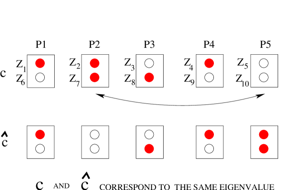
Figure 3: Example of two equivalent choice functions of the Bethe roots for the TASEP with $L=10$ and $N=5$.

The calculation of the degeneracies tables is therefore reduced to a pure problem in combinatorics : given a choice function $c$, one has to count the number of choice functions that are equivalent to $c$, and the total number of equivalence classes. Indeed, if we suppose that there is a ‘one to one’ bijection between choice sets and solutions of the Bethe Equations (recall that the number $\mathcal{N}$ of possible choice sets is the same as the dimension of the matrix $M$), then the following correspondences hold :

• equivalence classes by ‘package swapping’ $\leftrightarrow$ multiplets in spectrum

• cardinality of a class $\leftrightarrow$ order of the multiplet

• number of classes of cardinality $d$ $\leftrightarrow$ number of multiplets of degeneracy $d$.

In the half-filling case, the numbers in Table 1 are given by simple formulae (Golinelli and Mallick 2004b). The degeneracy order $d$ and the number $m(d)$ of multiplets of a given degeneracy $d$ can be expressed as a function of a single integer $r$

$$d_{r}=\left(\begin{array}[]{c}2r\\ r\end{array}\right),\,\,\,m(d_{r})=\left(\begin{array}[]{c}N\\ 2r\end{array}\right)2^{N-2r}\,,$$ (107)

where $r$ takes all integral values in the range $0\leq r\leq\frac{N}{2}\,.$ In arbitrary filling, expressions for $m$ and $d$ have also been found but they depend on $(L/\delta-1)$ different parameters (Golinelli and Mallick 2005b).

V Calculation of large deviation functions

The Bethe Ansatz has also led to an exact calculation of all the cumulants of the total current in the TASEP on a ring of size $L$ with $N$ particles (Derrida and Lebowitz 1998, Derrida and Appert 1999). As explained below, the generating function of these cumulants can be expressed as the ground state of a suitable deformation of the Markov matrix. From this generating function, the large deviation function of the time averaged current is obtained exactly.

V.1 A generalized master equation

We call $Y_{t}$ the total distance covered by all the particles between time 0 and time $t$ and define $P_{t}(\mathcal{C},Y)$ the joint probability of being at time $t$ in the configuration $\mathcal{C}$ and having $Y_{t}=Y$. A master equation, analogous to equation (1), can be written for $P_{t}(\mathcal{C},Y)$ as follows :

$$\frac{d}{dt}P_{t}(\mathcal{C},Y)=\sum_{\mathcal{C}^{\prime}}\Big{(}M_{0}(\mathcal{C},\mathcal{C}^{\prime})P_{t}(\mathcal{C}^{\prime},Y)+M_{1}(\mathcal{C},\mathcal{C}^{\prime})P_{t}(\mathcal{C}^{\prime},Y-1)+M_{-1}(\mathcal{C},\mathcal{C}^{\prime})P_{t}(\mathcal{C}^{\prime},Y+1)\Big{)}\,.$$ (108)

In terms of the generating function $F_{t}(\mathcal{C})$ defined as

$$F_{t}(\mathcal{C})=\sum_{Y=0}^{\infty}{\rm e}^{\gamma Y}P_{t}(\mathcal{C},Y)\,,$$ (109)

the master equation (108) takes the simpler form :

$$\frac{d}{dt}F_{t}(\mathcal{C})=\sum_{\mathcal{C}^{\prime}}\Big{(}M_{0}(\mathcal{C},\mathcal{C}^{\prime})+{\rm e}^{\gamma}M_{1}(\mathcal{C},\mathcal{C}^{\prime})+{\rm e}^{-\gamma}M_{-1}(\mathcal{C},\mathcal{C}^{\prime})\Big{)}F_{t}(\mathcal{C}^{\prime})=\sum_{\mathcal{C}^{\prime}}M(\gamma)(\mathcal{C},\mathcal{C}^{\prime})F_{t}(\mathcal{C}^{\prime})\,.$$ (110)

This equation is similar to the original Markov equation (1) for the probability distribution $P_{t}(\mathcal{C})$ but where the original Markov matrix $M$ is deformed into $M(\gamma)$ which is given by

$$M(\gamma)=M_{0}+{\rm e}^{\gamma}M_{1}+{\rm e}^{-\gamma}M_{-1}\,.$$ (111)

We emphasize that $M(\gamma)$, that governs the evolution of $F_{t}(\mathcal{C})$, is not a Markov matrix for $\gamma\neq 0$ (the sum of the elements in a given column does not vanish). In the long time limit, $t\to\infty$, the behaviour of $F_{t}(\mathcal{C})$ is dominated by the largest eigenvalue $\lambda(\gamma)$ of the matrix $M(\gamma)$ :

$$F_{t}(\mathcal{C})\to{\rm e}^{\lambda(\gamma)t}\langle\,\mathcal{C}\,|\,\lambda(\gamma)\,\rangle\,,$$ (112)

where the ket $|\lambda(\gamma)\rangle$ is the eigenvector corresponding to the largest eigenvalue. Therefore, when $t\to\infty$, we obtain

$$\langle\,{\rm e}^{\gamma Y_{t}}\,\rangle=\sum_{\mathcal{C}}F_{t}(\mathcal{C})\sim{\rm e}^{\lambda(\gamma)t}\,.$$ (113)

More precisely, we have

$$\lim_{t\to\infty}\frac{1}{t}\log\langle\,{\rm e}^{\gamma Y_{t}}\,\rangle=\lambda(\gamma)\,.$$ (114)

The function $\lambda(\gamma)$ contains the complete information about the cumulants of the total current $Y_{t}$ in the long time limit. The large deviation function $G(j)$ for the total current $j$ is defined as

$$G(j)=\lim_{t\to\infty}\frac{1}{t}\log\Big{[}{\rm Prob}\left(\frac{Y_{t}}{t}=j\right)\Big{]}\,.$$ (115)

The relation between $\lambda(\gamma)$ and $G(j)$ is derived as follows

$$\langle\,{\rm e}^{\gamma Y_{t}}\,\rangle\sim{\rm e}^{\lambda(\gamma)t}\sim\int{\rm e}^{t(G(j)+\gamma j)}{\rm d}j\,.$$ (116)

By saddle-point approximation, we deduce that $\lambda(\gamma)$ is the Legendre transform of $G(j)$

$$\lambda(\gamma)=\max_{j}\Big{(}G(j)+\gamma j\Big{)}\,.$$ (117)

This relation allows one to obtain the large deviation function $G(j)$ in the following parametric form, once $\lambda(\gamma)$ is known :

$$j=\frac{{\rm d}\lambda}{{\rm d}\gamma}\,\,\,\,\hbox{ and }\,\,\,\ G(j)=\lambda(\gamma)-\gamma\frac{{\rm d}\lambda}{{\rm d}\gamma}\,.$$ (118)

The largest eigenvalue $\lambda(\gamma)$ of the deformed matrix $M(\gamma)$ is calculated by Bethe Ansatz. The Bethe equations now read

$$z_{l}^{L}=(-1)^{N-1}\prod_{i=1}^{N}\frac{p{\rm e}^{\gamma}z_{l}z_{i}-z_{l}+q{\rm e}^{-\gamma}}{p{\rm e}^{\gamma}z_{l}z_{i}-z_{i}+q{\rm e}^{-\gamma}}\,\,\,{\rm for}\,\,\,\,l=1\ldots N\,,$$ (119)

and the corresponding eigenvalue of $M(\gamma)$ is given by

$$E(\gamma;z_{1},z_{2}\ldots z_{N})=p{\rm e}^{\gamma}\sum_{i=1}^{N}z_{i}+q{\rm e}^{-\gamma}\sum_{i=1}^{N}\frac{1}{z_{i}}-N\,.$$ (120)

V.2 The Gallavotti-Cohen symmetry

We remark that the equations (119) and (120) are invariant under the transformation

$$z \rightarrow \frac{1}{z}$$

$$\gamma \rightarrow \gamma_{0}-\gamma\,\,\,\,\hbox{ with }\,\,\,\,\gamma_{0}=\log\frac{q}{p}\,.$$ (121)

This symmetry implies that the spectrum of $M(\gamma)$ and that of $M(\gamma_{0}-\gamma)$ are identical. This functional identity is in particular satisfied by the largest eigenvalue of $M$ and we have

$$\lambda(\gamma)=\lambda(\gamma_{0}-\gamma)\,.$$ (122)

Using equation (117), we deduce that this identity implies the following symmetry for the large deviation function

$$G(j)=G(-j)-\gamma_{0}j\,.$$ (123)

This relation is a special case of the general Fluctuation Theorem valid for systems far from equilibrium (Evans, Cohen and Morriss 1993; Evans and Searles 1994, Gallavotti and Cohen 1995). This relation, which manifests itself here as a symmetry of the Bethe equations, does not depend on the integrability of the system and can be derived from equation (110) directly (Kurchan 1998, Lebowitz and Spohn 1999).

V.3 The large-deviation function for the TASEP

In the TASEP case, the Bethe equations (119) are simpler and can be solved by using the procedure outlined in section IV.2. An exact power series expansion in $\gamma$ for $\lambda(\gamma)$ is obtained by eliminating the parameter $Y$ in the following two equalities :

$$\lambda(\gamma) = -N\sum_{k=1}^{\infty}\left(\begin{array}[]{c}kL-1\\ kN\end{array}\right)\frac{Y^{k}}{kL-1}\,,$$ (126)

$$\gamma = -\sum_{k=1}^{\infty}\left(\begin{array}[]{c}kL\\ kN\end{array}\right)\frac{Y^{k}}{kL}\,.$$ (129)

Equation (129) is inverted by writing $Y$ formally as a power series in $\gamma$ and solving recursively for the coefficients up to any desired order; the function $\lambda(\gamma)$ is then obtained by substituting $Y(\gamma)$ in equation (126).

These expressions allow to calculate the cumulants of $Y_{t}$, for example :

$$\lim_{t\to\infty}\frac{\langle Y_{t}\rangle}{t} = \frac{{\rm d}\lambda(\gamma)}{{\rm d}\gamma}\Big{|}_{\gamma=0}=\frac{N(L-N)}{L-1}\,,$$ (130)

$$\,\,\,\lim_{t\to\infty}\frac{\langle Y_{t}^{2}\rangle-\langle Y_{t}\rangle^{2}}{t} = \frac{{\rm d}^{2}\lambda(\gamma)}{{\rm d}\gamma^{2}}\Big{|}_{\gamma=0}=\frac{N^{2}\;(2L-3)!\;(N-1)!^{2}\;(L-N)!^{2}}{(L-1)!^{2}\;(2N-1)!\;(2L-2N-1)!}\,.$$ (131)

In the limit of a large system size, $L\to\infty$, and with a fixed density $\rho=L/N$, these expressions reduce to

$$\lim_{t\to\infty}\frac{\langle Y_{t}\rangle}{t}\simeq L\rho(1-\rho)\,,\,\,\,\hbox{ and }\,\,\,\,\,\lim_{t\to\infty}\frac{\langle Y_{t}^{2}\rangle-\langle Y_{t}\rangle^{2}}{t}\simeq\frac{\sqrt{\pi}}{2}L^{3/2}[\rho(1-\rho)]^{3/2}\,.$$ (132)

Using the Stirling formula, equations (126) and (129) take the scaling form (Derrida and Lebowitz 1998)

$$\lambda(\gamma)-\gamma L\rho(1-\rho)=\sqrt{\frac{\rho(1-\rho)}{2\pi L^{3}}}\Phi\left(\gamma\sqrt{2\pi\rho(1-\rho)L^{3}}\right)\,,$$ (133)

where the expression for the scaling function $\Phi$ does not depend on the parameters ($L$ and $\rho$) of the model. From equation (133), it can be shown that when $|j-L\rho(1-\rho)|\ll L$, the large deviation function $G(j)$ can be written as

$$G(j)=\sqrt{\frac{\rho(1-\rho)}{\pi L^{3}}}H\Big{(}\frac{j-L\rho(1-\rho)}{\rho(1-\rho)}\Big{)}$$ (134)

with

$$H(y)\simeq-\frac{2\sqrt{3}}{5\sqrt{\pi}}y^{5/2}\,\,\,\, \,\,\,\,y\to+\infty\,,$$ for (135)

$$H(y)\simeq-\frac{4\sqrt{\pi}}{3}|y|^{3/2}\,\,\,\, \,\,\,\,y\to-\infty\,.$$ for (136)

This distribution is skew: it decays as a power law with an exponent $5/2$ for $y\to+\infty$ and with an exponent $3/2$ for $y\to-\infty$.

VI Applications to related models

In the previous sections, we have put emphasis on the Bethe Ansatz solution of the totally asymmetric exclusion process on a ring. In this special case, the Bethe equations have a particularly simple form and their analysis can be carried out thoroughly. In this last section, we briefly present results that have been obtained with the Bethe Ansatz for the partially asymmetric exclusion process (PASEP), for the exclusion process with an impurity, and for the exclusion process with open boundaries.

VI.1 The partially asymmetric exclusion process

The Bethe equations (74) for general hopping rates $p$ and $q$ can not be reduced to an effective one-variable polynomial equation as in the TASEP case and their analysis becomes much more involved. In particular, combinatorial expansions for the energy such as (97) valid for finite values of $L$ and $N$ are not known. However, a very thorough study has been carried out, in the limit $L\to\infty$, by Doochul Kim and his collaborators in a series of papers (Noh and Kim 1994, Kim 1995, Kim 1997, Lee and Kim 1999; see also related works on the non-Hermitian XXZ chain by Albertini et al. 1996, 1997). They developed a perturbative scheme that enabled them to calculate the finite size corrections of the gap and the low lying excitations of the asymmetric XXZ chain. They derived the crossover scaling functions of the energy gaps from the symmetric case $p=q=1/2$ to the asymmetric case. In the continuous limit, these functions describe a crossover from the Kardar-Parisi-Zhang universality class to the Edwards-Wilkinson class.

The same technique leads to the calculation of the large deviation function of the PASEP in the scaling limit (Lee and Kim 1999). The large deviation function takes the form

$$G(j)=(p-q)\sqrt{\frac{\rho(1-\rho)}{\pi N^{3}}}H\Big{(}\frac{j-L(p-q)\rho(1-\rho)}{(p-q)\rho(1-\rho)}\Big{)}$$ (137)

where the function $H$ is the same as that of equation (134). The only modification that occurs for the PASEP is the rescaling factor $p-q$. Non-trivial differences appear in the subleading terms, but these corrections are likely to be model-specific and non-universal. Using this expression of the large deviation function, it is possible to verify explicitly that the Gallavotti-Cohen relation (123) is satisfied (Lebowitz and Spohn 1999). However, an exact power series expansion of $\lambda(\gamma)$ in terms of the deformation parameter $\gamma$ is not known. Such an expansion would lead to exact formulae for the cumulants of the current valid for any values of $L$ and $N$. We believe, nevertheless, that expressions analogous to equations (126 and 129) should exist for the PASEP because exact combinatorial formulae for the mean value of the current and its variance have been calculated by using the Matrix Product method (Derrida and Mallick 1997).

VI.2 ASEP with an impurity

The presence of a defective particle (say, an impurity) in the ASEP on a ring can generate a shock dynamically in the stationary state (Mallick, 1996). A traffic-flow picture nicely illustrates this fact : if particles represent cars and the impurity a truck (which moves at a slower speed and is difficult to overtake), then the shock corresponds to a traffic jam. The phase transition to a shock can also be interpreted as a real space version of Bose-Einstein condensation (Evans 1996).

The model with a single defect particle is drawn in Figure 4. The system contains $N$ normal particles (denoted by 1) and one impurity (denoted by 2). Each site is either occupied by a particle or by the impurity, or it is empty. The stochastic dynamical rules that govern the evolution of the system during the infinitesimal time step $dt$ are

$$10 \rightarrow 01\,\,\,\,\,\hbox{ with rate }\,\,\,\,\,1$$

$$20 \rightarrow 02\,\,\,\,\,\hbox{ with rate }\,\,\,\,\,\alpha$$ (138)

$$12 \rightarrow 21\,\,\,\,\,\hbox{ with rate }\,\,\,\,\,\beta\,.$$

All other transitions are forbidden. The phase diagram of this model can be determined exactly by the Matrix product method and consists of four main phases (see Figure 4). In the two massive phases, the perturbation due to the impurity is of finite range and all correlations decay exponentially. In the non-massive phase, the impurity has a long range effect : correlations decay algebraically. In the shock phase, the presence of the unique impurity induces a phase separation between a low density region and a high density region.

By using the Bethe Ansatz, Derrida and Evans (1999) have calculated the large deviation function of the total displacement of the defect particle. Their result leads to analytical formulae for the velocity and the diffusion constant of the impurity in the various phases. In particular, in the shock phase, the location of the defect can be identified with the position of the shock and the large deviation function provides complete information on its statistical behaviour.

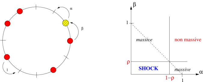
Figure 4: The Asymmetric exclusion process on a periodic ring with an impurity.

A more direct way to produce a shock in a system is to introduce a slow bond that particles cross with a rate $r<1$ (Janowski and Lebowitz 1992, 1994). For $r$ less than a critical value that depends on the mean density of particles, the system exhibits a phase separation. This model, in spite of many efforts, has not been solved exactly and is probably not an integrable system (it does not satisfy any known criterion for integrability). However, G. Schütz (1993) has solved, using Bethe Ansatz, a variant of this model in which particles move deterministically on a ring of length $L$ (with $L$ even) with a single defect across which the particles jump with probability $r<1$. In this dynamics, the time evolution consists of two intermediate time steps in which even sites and odd sites are updated simultaneously.

VI.3 The open boundary model

The asymmetric exclusion process with open boundaries can be viewed as a model for a driven lattice gas in contact with two reservoirs. In the bulk, the dynamics of the ASEP is the same as that shown in Figure 1; at the boundaries particles can enter or leave the system with various input/output rates. The totally asymmetric version of this model is illustrated in Figure 5 : particles in the bulk jump to to right with rate 1; a particle can be added with rate $\alpha$ if the site 1 is empty; a particle can be removed with rate $\beta$ if the site L is occupied.

The open ASEP undergoes boundary induced phase transitions (Krug 1991). The density profile and the current can be calculated exactly by using a Matrix product representation for the steady state (Derrida et al. 1993; see also Schütz and Domany 1993 for an alternative derivation). In the large system size limit, the expressions for the current and the density profile become non-analytic for certain values of the input/output rates. This leads to a phase diagram with three main regions : a low density phase (when typically the input rates are small and the output rates are large), a high density phase (when the input rates are large and the output rates small), and a maximal current phase (in which the bulk density is 1/2 regardless of the boundary rates).

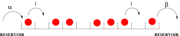
Figure 5: The Totally Asymmetric exclusion process on an open chain

Although the ASEP with open boundaries was known to be an integrable system (Essler and Rittenberg 1996), the explicit diagonalisation of the Markov matrix by Bethe Ansatz could not be carried out because of the boundary terms that violate the conservation of the total number of particles. Only numerical and phenomenological studies of the spectrum were available (Bilstein and Wehefritz 1997, Dudziński and Schütz 2000). In a remarkable recent paper, de Gier and Essler (2005) were able to derive the Bethe Ansatz equations describing the complete spectrum of the Markov matrix of the partially asymmetric exclusion process with open boundaries and general input/output rates. Their work uses an exact solution of the open XXZ chain with non-diagonal boundary terms (Nepomechie 2003 and 2004, Cao et al. 2003). De Gier and Essler have calculated analytically the spectral gap of the TASEP with open boundaries and have discussed the various regimes throughout the phase diagram; in particular they have discovered a fine structure of the phase diagram that could not be found from the stationary state alone. Their work opens the way to many further investigations, such as the description of the excited states and the calculation of the large deviation function of the current in the open system.

VII Conclusion

The Bethe Ansatz was initially used to diagonalize Quantum Hamiltonians (such as the Heisenberg Spin Chain, the one-dimensional Bose gas with $\delta$-interactions) and to calculate real spectra of Hermitian Operators. In the 70’s and the beginning of the 80’s, the exact solutions of the six and eight vertex models and the development of the quantum inverse scattering method (Baxter 1982, Faddeev 1984) showed that many systems of interest in equilibrium statistical mechanics belonged to the class of integrable models. The ASEP, which plays the role of a paradigm in non-equilibrium statistical mechanics, thanks to its rich and complex phenomenology, has been shown to be integrable. This integrability property has allowed to derive many exact solutions for the ASEP and for some related models that we have reviewed here. These analytical results add to our knowledge of systems far from equilibrium and allow us to compare them with systems at equilibrium on a quantitative level.

The use of integrability techniques in non-equilibrium statistical mechanics is an active field of current research. In particular, we believe that the following problems should lead to interesting results in near future : the use of the nested Bethe Ansatz for ASEP with multiple species of particles, the investigation of ASEP with open boundaries, the study of exclusion processes with disorder, and the application of integrability techniques to the zero-range process (Povolotsky 2004, Povolotsky and Mendes 2006)

Acknowledgments

We wish to thank the guest editors of this special issue, Patrick Dorey, Gerald Dunne and Joshua Feinberg for inviting us to write this contribution. We are particularly thankful to Patrick Dorey for his encouragements and his patience. We thank B. Derrida, M. Gaudin, V. Hakim, T. Jolicœur, S. Majumdar, S. Nechaev, V. Pasquier, G. Schütz, H. Spohn, R. Stinchcombe and V. Rittenberg for useful discussions. We are particularly greatful to S. Mallick for a critical reading of the manuscript. We thank the anonymous referee for many very helpful comments.

References

• G. Albertini, S. R. Dahmen, B. Wehefritz, 1996, Phase diagram of the non-Hermitian asymmetric XXZ spin chain, J. Phys. A: Math. Gen. 29, L369.

• G. Albertini, S. R. Dahmen, B. Wehefritz, 1997, The free energy singularity of the asymmetric 6-vertex model and the excitations of the asymmetric XXZ chain, Nucl. Phys. B 493 541.

• F. C. Alcaraz, M. Droz, M. Henkel, V. Rittenberg, 1994, Reaction-diffusion processes, critical dynamics, and quantum chains, Ann. Phys. 230, 250.

• F. C. Alcaraz, M. J. Lazo, 2004, The Bethe Ansatz as a matrix product Ansatz, J. Phys. A: Math. Gen. 37, L1-L7

• R. J. Baxter, 1982 Exactly solvable models in Statistical Mechanics (Academic Press, San Diego).

• H. Bethe, 1931, Zur Theory der Metalle. I Eigenwerte und Eigenfunctionen Atomkette Zur Physik 71, 205.

• U. Bilstein, B. Wehefritz, 1997, Spectra of non-Hermitian quantum spin chains describing boundary induced phase transitions, J. Phys. A: Math. Gen. 30, 4925.

• R. Bundschuh, 2002, Asymmetric exclusion process and extremal statistics of random sequences, Phys. Rev. E 65, 031911.

• J. Cao, H.-Q. Lin, K.-J. Shi, Y. Wang, 2003, Exact solution of XXZ spin chain with unparallel boundary fields, Nucl. Phys. B. 663, 487.

• B. Derrida, 1998, An exactly soluble non-equilibrium system: the asymmetric simple exclusion process, Phys. Rep. 301, 65.

• B. Derrida, C. Appert, 1999, Universal large-deviation function of the Kardar-Parisi-Zhang equation in one dimension, J. Stat. Phys. 94, 1.

• B. Derrida, M. R. Evans, 1999, Bethe Ansatz solution for a defect particle in the asymmetric exclusion process, J. Phys. A: Math. Gen. 32, 4833.

• B. Derrida, M. R. Evans, V. Hakim, V. Pasquier, 1993, Exact solution of a 1D asymmetric exclusion model using a matrix formulation, J. Phys. A: Math. Gen. 26, 1493.

• B. Derrida, J. L. Lebowitz, 1998, Exact large deviation function in the asymmetric exclusion process, Phys. Rev. Lett. 80, 209.

• B. Derrida, J. L. Lebowitz, E. R. Speer, 2003, Exact large deviation functional of a stationary open driven diffusive system: the asymmetric exclusion process, J. Stat. Phys. 110, 775.

• B. Derrida, K. Mallick, 1997, Exact diffusion constant for the one-dimensional partially asymmetric exclusion process, J. Phys. A: Math. Gen. 30, 1031.

• D. Dhar, 1987, An exactly solved model for interfacial growth, Phase Transitions 9, 51.

• M. Dudziński, G. M. Schütz, 2000, Relaxation spectrum of the asymmetric exclusion process with open boundaries, J. Phys. A: Math. Gen. 33, 8351.

• F. H. Essler, V. Rittenberg, 1996 Representations of the quadratic algebra and partially asymmetric diffusion with open boundaries, J. Phys. A: Math. Gen. 29, 3375.

• M. R. Evans, 1996, Bose-Einstein condensation in disordered exclusion models and relation to traffic flow, Europhys. Lett. 36, 13.

• D. J. Evans, E. G. D. Cohen, G. P. Morriss, 1993 Probability of Second Law Violations in Shearing Steady states, Phys. Rev. Lett. 71, 2401.

• D. J. Evans, D. J. Searles, 1994 Equilibrium microstates which generate second law violating steady states, Phys. Rev. E 50, 1645.

• L. D. Faddeev, 1984, Integrable models in 1+1 dimensional quantum field theory, in Les Houches Lectures 1982 (Elsevier).

• G. Gallavotti, E. G. D. Cohen, 1995 Dynamical ensembles in non-equilibrium statistical mechanics, Phys. Rev. Lett. 74, 2694; Dynamical ensembles in stationary states, J. Stat. Phys 80 931.

• J. de Gier, F. H. L. Essler, 2005, Bethe Ansatz solution of the Asymmetric Exclusion Process with Open Boundaries, Phys. Rev. Lett. 95, 240601.

• O. Golinelli, K. Mallick, 2004a, Bethe Ansatz calculation of the spectral gap of the asymmetric exclusion process, J. Phys. A: Math. Gen. 37, 3321.

• O. Golinelli, K. Mallick, 2004b, Hidden symmetries in the asymmetric exclusion process, J. Stat. Mech.: Theor. Exp. P12001468/2004/12/P12001.

• O. Golinelli, K. Mallick, 2005a, Spectral gap of the totally asymmetric exclusion process at arbitrary filling, J. Phys. A: Math. Gen. 38 1419.

• O. Golinelli, K. Mallick, 2005b, Spectral Degeneracies in the Totally Asymmetric Exclusion Process, J. Stat. Phys 120 779.

• O. Golinelli, K. Mallick, 2006, Derivation of a matrix product representation for the asymmetric exclusion process from Algebraic Bethe Ansatz, J. Phys. A: Math. Gen. 39 10647.

• L.-H. Gwa, H. Spohn, 1992, Bethe solution for the dynamical-scaling exponent of the noisy Burgers equation, Phys. Rev. A 46, 844.

• T. Halpin-Healy, Y.-C. Zhang, 1995, Kinetic roughening phenomena, stochastic growth, directed polymers and all that, Phys. Rep. 254, 215.

• S. A. Janowski, J. L. Lebowitz, 1992 Finite size effects and Shock fluctuations in the asymmetric exclusion process, Phys. Rev. A 45, 618.

• S. A. Janowski, J. L. Lebowitz, 1994 Exact results for the asymmetric exclusion process with a blocage, J. Stat. Phys. 77, 35.

• D. Kandel, E. Domany, B. Nienhuis, 1990, A six-vertex model as a diffusion problem: derivation of correlation functions, J. Phys. A: Math. Gen. 23, L755.

• S. Katz, J. L. Lebowitz, H. Spohn, 1984, Nonequilibrium steady states of stochastic lattice gas models of fast ionic conductors, J. Stat. Phys. 34, 497.

• D. Kim, 1995, Bethe Ansatz solution for crossover scaling functions of the asymmetric XXZ chain and the Kardar-Parisi-Zhang-type growth model, Phys. Rev. E 52, 3512.

• D. Kim, 1997, Asymmetric XXZ chain at the antiferromagnetic transition: spectra and partition functions, J. Phys. A: Math. Gen. 30, 3817.

• S. Klumpp, R. Lipowsky, 2003, Traffic of molecular motors through tube-like compartments, J. Stat. Phys. 113, 233.

• J. Krug, 1991, Boundary-Induced Phase Transitions in Driven Diffusive Systems, Phys. Rev. Lett. 67, 1882.

• J. Krug, 1997, Origins of scale invariance in growth processes, Adv. Phys. 46, 139.

• J. Kurchan, 1998, Fluctuation theorem for stochastic dynamics, J. Phys. A: Math. Gen. 31, 3719.

• J. L. Lebowitz, H. Spohn, 1999 A Gallavoti-Cohen type symmetry in the large deviation functional for stochastic dynamics, J. Stat. Phys. 95, 333.

• D. S. Lee, D. Kim, 1999, Large deviation function of the partially asymmetric exclusion process, Phys. Rev. E 59, 6476.

• D. G. Levitt, 1973, Dynamics of a single-file pore: Non-Fickian behavior, Phys. Rev. A 8, 3050.

• T. M. Liggett, 1985, Interacting Particle Systems, (Springer-Verlag, New-York).

• T. M. Liggett, 1999, Stochastic Models of Interacting Systems:Contact, Voter and Exclusion Processes, (Springer-Verlag, New-York).

• C. T. MacDonald, J. H. Gibbs, A. C. Pipkin, 1968, Kinetics of biopymerization on nucleic acid templates, Biopolymers 6, 1.

• C. T. MacDonald, J. H. Gibbs, 1969, Concerning the kinetics of polypeptide synthesis on polyribosomes, Biopolymers 7, 707.

• K. Mallick, 1996, Shocks in the asymmetric exclusion model with an impurity, J. Phys. A: Math. Gen. 29, 5375.

• R. I. Nepomechie, 1999, A spin Chain Primer, Int.J.Mod.Phys.B 13, 2973.

• R. I. Nepomechie, 2003, Functional Relations and Bethe Ansatz for the XXZ Chain, J. Stat. Phys. 111, 1363.

• R. I. Nepomechie, 2004, Bethe Ansatz solution of the open XXZ chain with nondiagonal boundary terms, J. Phys. A: Math. Gen. 37, 433.

• J. D. Noh, D. Kim, 1994, Interacting domain walls and the five-vertex model, Phys. Rev. E 49, 1943.

• A. M. Povolotsky, 2004, Bethe Ansatz solution of zero-range process with nonuniform stationary state, Phys. Rev. E 69, 061109.

• A. M. Povolotsky, J. F. F. Mendes, 2006, Bethe ansatz solution of discrete time stochastic processes with fully parallel update, to appear in J. Stat. Phys.

• V. B. Priezzhev, 2003, Exact Nonstationary Probabilities in the Asymmetric Exclusion Process on a Ring, Phys. Rev. Lett. 91, 050601.

• A. Rákos, G. M. Schütz, 2005, Bethe Ansatz and current distribution for the TASEP with particle-dependent hopping rates, cond-mat/0506525

• P. M. Richards, 1977, Theory of one-dimensional hopping conductivity and diffusion, Phys. Rev. B 16, 1393.

• T. Sasamoto, M. Wadati, 1998, Exact results for one-dimensional totally asymmetric diffusion models, J. Phys. A: Math. Gen. 31, 6057.

• B. Schmittmann and R. K. P. Zia, 1995, Statistical mechanics of driven diffusive systems, in Phase Transitions and Critical Phenomena vol 17., C. Domb and J. L. Lebowitz Ed., (San Diego, Academic Press).

• M. Schreckenberg, D. E. Wolf (ed.), 1998, Traffic and granular flow ’97 (Springer-Verlag, New-York).

• G. M. Schütz, 1993, Generalized Bethe Ansatz solution of a one-dimensional asymmetric exclusion process on a ring with blockage, J. Stat. Phys. 71, 471.

• G. M. Schütz, 1997, Exact solution of the master equation of the asymmetric exclusion process, J. Stat. Phys. 88, 427.

• G. M. Schütz, 2001, Exactly Solvable Models for Many-Body Systems Far from Equilibrium in Phase Transitions and Critical Phenomena vol 19., C. Domb and J. L. Lebowitz Ed., (Academic Press, San Diego).

• E. R. Speer, 1993, The two species totally asymmetric exclusion process, in Micro, Meso and Macroscopic approaches in Physics, M. Fannes C. Maes and A. Verbeure Ed. NATO Workshop ’On three levels’, Leuven, July 1993.

• F. Spitzer, 1970, Interaction of Markov Processes, Adv. in Math. 5, 246.

• H. Spohn, 1991, Large scale dynamics of interacting particles, (Springer-Verlag, New-York).

• R. Stinchcombe   G. M. Schütz, 1995, Application of Operator algebras to stochastic dynamics and the Heisenberg chain, Phys. Rev. Lett. 75, 140.

• H. J. de Vega, 1989, Yang-Baxter algebras, integrable theories and quantum groups, Int. Jour. Mod. Phys. A 4, 2371.

• B. Widom, J. L. Viovy, A. D. Defontaines, 1991, Repton model of gel electrophoresis and diffusion, J. Phys. I France 1, 1759.