Phase diagram of an Ising model with competitive interactions on a Husimi tree and its disordered counterpart

Abstract

We consider an Ising competitive model defined over a triangular Husimi tree where loops, responsible for an explicit frustration, are even allowed. After a critical analysis of the phase diagram, in which a “gas of non interacting dimers (or spin liquid) - ferro or antiferromagnetic ordered state” transition is recognized in the frustrated regions, we introduce the disorder for studying the spin glass version of the model: the triangular $\pm J$ model. We find out that, for any finite value of the averaged couplings, the model exhibits always a phase transition, even in the frustrated regions, where the transition turns out to be a glassy transition. The analysis of the random model is done by applying a recently proposed method which allows to derive the upper phase boundary of a random model through a mapping with a corresponding non random one.

1 Introduction

Models of statistical mechanics defined over Bethe lattices [1] constitute a framework that, due to two peculiar ingredients, namely exact solvability and finite connectivity, as opposed to unsolvability of finite dimensional models (for $D>2$) or to exact solvability of models defined over the fully connected graph (mean field), sheds some light toward the understanding of more realistic models. It is in fact believed that several thermal properties of the model could persist for regular lattices as well. Nowadays, the emerging science of networks has attracted a renewed interested in such models [2, 3, 4, 5]. In fact, roughly speaking one can say that the Bethe lattice represents the simplest prototype of network where an exact solution is often accessible. At least for uncorrelated random networks, it has been indeed proved that, if we indicate with $<f(q)>$ the average over the network of some function $f$ of the vertex degree $q$, the critical behavior of a given model with positive couplings defined over a Bethe lattice of degree $q_{B}$, coincides with that defined over the network provided that an effective substitution $q_{B}\rightarrow<q^{2}>/<q>$ for taking into account of the distribution of link ends rather than that of links, is performed [6, 7].

As is known, the exact solvability of a model defined over a Bethe lattice relies on the fact that the lattice is a tree, i.e., a graph without loops [1]. However, in relatively recent years progresses have been made in facing, analytically, models defined over lattices in which a finite number of closed paths per vertex is also allowed [8, 9], which we refer as “generalized tree-like structures”, see Fig. 1, and models defined over graphs in which the tree-like structure is partially broken due to the presence of an infinite number of closed paths per vertex as happens in generalized Bethe lattices (see for example [10] and references therein) and in Husimi trees [11, 12, 13, 14, 15, 16, 17]. The graph depicted in Fig. 2 is an example of a Husimi tree.

Figure 1: An example of a generalized tree-like graph.

Figure 2: The graph over which the competitive model of Eq. 1 is defined: a triangular Husimi tree. The continuous segments constitute a Bethe lattice $\Gamma$ (an infinite tree). Dashed segments connect vertices of $\Gamma$ belonging to the same shell. Note that, a part the root 0, the degree of $\Gamma$ is $q_{\Gamma}=3$, whereas the degree of the Husimi tree is $q_{\Gamma}^{\prime}=4$.

Notice that, by definition, in a loop both vertices and bonds repetitions are forbidden, whereas in a closed path only bonds repetitions are forbidden; in a closed path a same vertex can be crossed more than one time. So that, for example, in the graph of Fig. 1, and in a regular $D$-dimensional lattice with $D>1$ or in the graph of Fig. 2, the number of loops per vertex is finite, but the number of closed paths per vertex is finite only in the graph of Fig. 1. This kind of difference reflects on the different complexities in solving models defined on generalized tree-like structures and non tree-like structures; whereas the first class of problems can be exactly faced in the framework of a suitable Bethe-Peierls approach (see for example the reviews [18, 19] ) or, alternatively, by using the rules given in the Refs. [8, 9] for determining the critical surfaces, for the second class of problems, in general, a closed analytical method is lacking. An exception to this is provided by models defined over generalized Bethe lattices and Husimi trees. For these models in fact, the problem of statistical mechanics can be mapped on a that of a dynamical system involving few degrees of freedom [10, 11]. In particular, the model defined over the Husimi tree of Fig. 2, which is the subject of this paper, can be solved analytically in a closed form.

In these kind of relatively solvable models, one is usually interested in studying competition effects, so that two or more independent couplings $J_{\mathrm{1}},J_{\mathrm{2}},\ldots$ along the links of the lattice are given. As already investigated by numerical and semi-analytical methods, not only on generalized Bethe lattices and Husimi trees [11, 20, 21, 22, 23, 10, 24], but even on finite dimensional lattices [25, 26], due to the competitiveness in amplitude and sign of the couplings and to the presence of loops giving rise to frustration [27], a quite rich scenario of phases can take place. In fact, besides ferro and antiferromagnetism, competing interactions lie at the heart of a variety of original phenomena in magnetic systems, including the existence of modulated [10] and spin glass phases [28].

After the study of the Ising and the Potts competitive models [13, 15, 16, 11] defined over generalized Bethe lattices and Husimi trees with a uniform or periodic distribution of the couplings $J_{\mathrm{1}},J_{\mathrm{2}},\ldots$, the next natural step toward the complexity of these competitive models is the introduction of disorder. We present here a twofold study of the simpler Ising model with two competitive interactions $J_{\mathrm{1}}$ and $J_{\mathrm{2}}$ defined over the triangular Husimi tree of Fig. 2. We first review this model giving the proper interpretation of the phases in terms of the magnetization. Then we introduce the disorder to study the triangular $\pm J$ model. To this aim, we let $J_{\mathrm{1}}$ and $J_{\mathrm{2}}$ to be random couplings having a discrete probability distribution whose spread, i.e., the measures of the disorder, is characterized by two parameters, $p_{1}$ and $p_{2}$. The analysis of the phase diagram of the random model is done by using an effective method recently developed in [29] and already used in [30]. This method consists on a mapping between the phase diagram of the random model and the corresponding non random one. In [29] it has been shown that, in the thermodynamic limit, the upper phase boundary of the random model one finds by using this mapping, as well as the corresponding critical behavior, become exact whenever the graph over which the model is defined turns out to be infinite dimensional in a broad sense, as happens for instance in generalized tree-like structures or generalized Bethe lattices and Husimi trees. Unlike what emphasized in a previous version of this manuscript however, we stress here that Bethe lattices (here meant as infinite trees) and Husimi trees represent a limit case where the mapping in general is not well defined. In fact, the mapping can establish a correspondence between the random model and a corresponding non random one, both built up over the same graph, only if their density free energies exist (more precisely the non trivial part of the density free energy, see Eq. (12)). We refer the reader to the recent work [31] for a rigorous formulation of the mapping. It happens unfortunately that, due to the problem of the boundary conditions (see also the discussion in Appendix), which in a Bethe lattice and in a Husimi tree constitute a finite fraction of the total size of the system, in a Bethe lattice (here meant as an infinite tree) and in a Husimi tree, the density free energy, as a proper thermodynamic limit, does not exist (however the circumstances for a Bethe lattice is in some sense fortunate and the mapping turns out exact). Therefore we advise the reader that the results we report in this manuscript cannot be taken as exact; they have to be considered as a mere application of the mapping being here formal and not rigorous. Nevertheless, the equations of the mapping are still defined and, as an approximation, they can be applied in a Husimi tree case as well. In fact, in studying another random version of the model, the diluted frustrated model, in which the disorder is introduced by randomly deleting the negative couplings $J_{2}$ with some probability $\mu$, we have found some differences between the results one can obtain by applying the mapping and the results one can find by using a Bethe-Peierls-like approach [32]. It turns out that, in the limit $0<-J_{2}\ll J_{1}$, this latter method succeeds in giving the exact percolation threshold $\mu_{P}=1/\sqrt{2}$, while the mapping gives $\mu_{P}=\sqrt{3}-1$; and a larger difference is observed in the opposite limit $-J_{2}\gg J_{1}>0$. Nevertheless we think that the application of the mapping also in the Husimi tree cases provides easily important information of the random model. We stress in fact that in the mapping no ad hoc approximation, like the local tree-like approximation, is introduced.

For the present model, Eqs. (1-6), we have found the following scenario. Concerning the magnetization, in the non random model in the frustrated regions there is no phase transition for $|J_{2}|>|J_{1}|$ even at $T=0$, and this is physically explained by looking directly at the ground state that becomes equivalent to a gas of non interacting dimers with coupling $J_{2}$ (also called a spin liquid in the literature). In the $\pm J$ triangular model instead, even for $p_{1}=p_{2}=1$, there exists always a stable spin glass transition and, for suitable values of $p_{1}$ and $p_{2}$ a ferro or antiferromagnetic disordered transition may exist as well. Whereas the latter transition can be read just as due to an effective renormalization of the couplings $J_{1}$ and $J_{2}$, the former transition is interpreted as due to the onset of the overlap ordering of the dimers, as signaled by the study of the exact ground states of the non random model which is equivalent to the random one for $p_{1}=p_{2}=1$. Furthermore, we observe that in the limit $|J_{2}|\gg|J_{1}|$ the picture in terms of non interacting dimers is recovered also in the glassy phase.

We shall limit ourself mainly to the study of the critical surfaces inferring little on the nature of the several phases. Furthermore, we recall that for negative couplings, the correspondence between the solution of the Ising model on the Bethe lattice (the graph of Fig. 2 with $J_{2}=0$) and that on a corresponding sparse system (like the Erd$\mathrm{\ddot{o}}$s R$\mathrm{\acute{e}}$nyi random graph), where long global frustrated loops are also present, is lost. Therefore, following the same philosophy of, e.g., the Refs. [20, 21, 10], the solution we will present here concerns, strictly speaking, only an Ising model model defined over a structure where global loops are absent. Nevertheless, we believe that since we take into account the effect of all the other explicit loops, at least for certain aspects, the solution we find sheds some light also on a possible sparse representation of the model even in the frustrated regions. In fact, the ground state we describe in Sec. 3 has a quite strong similarity to that one finds in the anisotropic triangular Ising model [34].

The competitive non random model was partially already analyzed in [13, 15, 32]. Notice that it is different from the model considered in the Ref. [11] (third item); in fact, in the non random case, its relative simplicity allows an exact analytical study. Note also that in the Refs. [13, 15, 32] no detail about the ground states was given.

Very recently, a renewed attention has been attracted by the role of loops both in statistical mechanics and computer science [35, 36, 37, 38]. In fact, even if the most used Bethe-Peierls approximation usually works well in many important models near to be tree-like, rigorously speaking, it becomes exact only in perfect tree-structures and generalized tree-like structures, like the one depicted in Fig. 1, whereas in more complex graphs like that of Fig. 2, can be wrong. Successful efforts have been made toward a general treatment of the problem and systematic corrections to the Bethe-Peierls approximation have been now rigorously established [39]. However, as a general rule, we recall that between the complexity, both analytical or numerical, in solving a random model and a corresponding non random one there is a gap. In fact, in general the approach used to solve, possibly exactly, the latter, does not lend itself to be simply adapted to the former. Our study, even if limited to the knowledge of the upper critical surface and to the critical behavior, constitutes an example of a general procedure which, at least in the cases where the conditions for the mapping are satisfied, covers this gap.

The paper is organized as follows. In Sec. 2 we introduce the uniform and the random model defined over the triangular Husimi tree of Fig. 2. In Sec. 3 we analyze the phase diagram of the uniform model giving the proper interpretation of the invariant ground states. In Sec. 4 we recall the mapping through which the phase diagram of the random model will be analyzed in the following Sec. 5. Finally, some conclusions are drawn in Sec. 4. The Appendix A is devoted to Sec. 3.

2 Competitive Ising models on a structure with loops

Let us consider a semi-infinite Bethe lattice $\Gamma$ in which any vertex, but a singular one 0, has coordination number $q_{\Gamma}=3$ (i.e. branching number $k=2$) as in Fig. 2. Chosen $0$ as a root vertex, it is convenient to divide $\Gamma$ in shells $S_{1},S_{2},\ldots,S_{n},\ldots$ [1]. Given a couple of vertices $(x,y)$ of $\Gamma$, we will write $(x,y)$ as $<x,y>$ if $x$ and $y$ are nearest neighbors, i.e., if they are connected through a bond of $\Gamma$, and $(x,y)$ as $>x,y<$ if $x$ and $y$ belong to the same shall $S_{n}$ and are at distance $d(x,y)=2$ on $\Gamma$.

2.1 Non random case

Let us consider the following Ising model with competing interactions

$$H(\sigma)=-J_{\mathrm{1}}\sum\limits_{<x,y>}{\sigma(x)\sigma(y)}-J_{\mathrm{2}}\sum\limits_{>x,y<}{\sigma(x)\sigma(y)}$$ (1)

where $J_{\mathrm{1}},J_{\mathrm{2}}\in\mathop{\mathrm{R}}$ are coupling constants and $\sigma$ is a configuration of spin variables $\sigma_{x}=\pm 1$ over the vertices of $\Gamma$. Far from the root the graph over which this Ising model is defined, is characterized by the fact that at any vertex is present a triangular loop with two couplings $J_{\mathrm{1}}$ and one coupling $J_{\mathrm{2}}$ as indicated in Fig. 2. For $J_{2}\neq 0$ the model is defined over the Husimi tree of Fig. 2 having degree $q_{\Gamma}^{\prime}=4$.

2.2 Random case (spin glass)

In the random version of the competitive model of Eq. (1), the couplings $J_{\mathrm{1}}$ and $J_{\mathrm{2}}$ become independent random variables so that the corresponding Hamiltonian for the quenched system is

$$H(\sigma)=-\sum\limits_{<x,y>}J_{x,y}^{(1)}{\sigma(x)\sigma(y)}-\sum\limits_{>x,y<}J_{x,y}^{(2)}{\sigma(x)\sigma(y)}.$$ (2)

The free energy $F$ is defined by

$$-\beta F\equiv\int d\mathcal{P}\left(\{J_{x,y}^{(1)}\},\{J_{x,y}^{(2)}\}\right)\log\left(Z\left(\{J_{x,y}^{(1)}\},\{J_{x,y}^{(2)}\}\right)\right),$$ (3)

where $Z\left(\{J_{x,y}^{(1)}\},\{J_{x,y}^{(2)}\}\right)$ is the partition function of the quenched system and $d\mathcal{P}\left(\{J_{x,y}^{(1)}\},\{J_{x,y}^{(2)}\}\right)$ is a product measure given by

$$d\mathcal{P}\left(\{J_{x,y}^{(1)}\},\{J_{x,y}^{(2)}\}\right)=\prod_{<x,y>}d\mu_{\mathrm{1}}\left(J_{x,y}^{(1)}\right)\prod_{>x,y<}d\mu_{\mathrm{2}}\left(J_{x,y}^{(2)}\right),$$ (4)

$d\mu_{\mathrm{1}}$ and $d\mu_{\mathrm{2}}$ being two given normalized measures featuring the disorder. In general this model, besides a disordered ferromagnetic or antiferromagnetic transition (P-F/AF), may manifest a spin glass transition (P-SG). A generic inverse critical temperature of the random model will be indicated by $\beta_{c}$. We will consider the following choice:

2.2.1 Triangular $\pm J$ model

$$d\mu_{\mathrm{1}}\left(J_{x,y}^{(1)}\right) = p_{\mathrm{1}}\delta(J_{x,y}^{(1)}-J_{\mathrm{1}})+(1-p_{\mathrm{1}})\delta(J_{x,y}^{(1)}+J_{\mathrm{1}}),$$ (5)

$$d\mu_{\mathrm{2}}\left(J_{x,y}^{(2)}\right) = p_{\mathrm{2}}\delta(J_{x,y}^{(2)}-J_{\mathrm{2}})+(1-p_{\mathrm{2}})\delta(J_{x,y}^{(2)}+J_{\mathrm{2}}),$$ (6)

where $J_{\mathrm{1}}$ and $J_{\mathrm{2}}$, as in the non random model, are arbitrary parameters and $p_{\mathrm{1}},p_{\mathrm{2}}\in[0,1]$ characterize the disorder, maximum at $p_{\mathrm{1}}=p_{\mathrm{2}}=0.5$ and minimum for $p_{\mathrm{1}}$ and $p_{\mathrm{2}}$ equal to 0 or 1.

3 Analysis of the non random model: phase diagram - gas of dimers

Concerning the phase transitions, the model defined in Sec. 2.1, even in the presence of an external magnetic field $h$, has been recently solved analytically in [13]. In Appendix A we report another approach for deriving the phase transitions. There are two critical lines given by

$$\theta_{\mathrm{2}}=\frac{2\theta_{\mathrm{1}}}{\theta_{\mathrm{1}}^{2}-3},\quad\theta_{\mathrm{1}}>\sqrt{3},$$ (7)

$$\theta_{\mathrm{2}}=\frac{2\theta_{\mathrm{1}}}{1-3\theta^{2}_{\mathrm{1}}},\quad\theta_{\mathrm{1}}<1/\sqrt{3},$$ (8)

where the parameters $\theta_{\mathrm{1}}$ and $\theta_{\mathrm{2}}$ are defined as

$$\theta_{\mathrm{1}}=e^{2\beta J_{\mathrm{1}}},\quad\theta_{\mathrm{2}}=e^{2\beta J_{\mathrm{2}}}.$$ (9)

In Fig. 3 we show the corresponding phase diagrams obtained as solutions of Eqs. (7) and (8) along the axis $T/J_{\mathrm{1}}$ and $J_{\mathrm{2}}/J_{\mathrm{1}}$. Equations (7) and (8) describe, respectively, a paramagnetic-ferromagnetic (P-F) transition, in which $J_{1}>0$, and a paramagnetic-antiferromagnetic (P-AF) transition in which $J_{1}<0$. By a direct inspection of the minimum of $H$, Eq. (1), it follows that, in the two non paramagnetic frustrated (Fr) regions $J_{1}>0,J_{2}<0$ and $J_{1}<0,J_{2}<0$, see Fig. 3, the corresponding ground states, despite the frustration, are simply F and AF, respectively. The reason for that lies on the smallness (in modulo) of the coupling $J_{2}$ in the two mentioned regions. More precisely, by looking at the configurations minimizing the energy, it is easy to see that, if e.g. $J_{1}>0$ and $J_{2}<0$, for $J_{1}>|J_{2}|$ there exist only two ground states obtained by taking all the spins parallel, the corresponding ground state energy per triangle being $e=-2J_{1}-J_{2}$ (see Fig. 4); whereas for $J_{1}<|J_{2}|$ the ground state becomes infinitely degenerate, the corresponding ground state energy per triangle being $e^{\prime}=J_{2}$ (see Fig. 5). In the latter case the whole set of ground states is obtained by taking in all the possible ways the spins connected by the couplings $J_{2}$ (i.e., the spins on the same shell at distance $d=2$ on $\Gamma$) as antiparralel. A similar conclusion holds also in the other frustrated region where $J_{1},J_{2}<0$. In this case, when $|J_{1}|>|J_{2}|$, the ground state is obtained by taking alternated spins on the Bethe lattice $\Gamma$ (note that, as a consequence, the spins are not alternated on the Husimi tree; spins on the same shall are parallel, see Fig. 6); whereas for $|J_{1}|<|J_{2}|$ the ground state has the same structure of the case $J_{1}>0$ and $|J_{1}|<|J_{2}|$ above analyzed (Fig. 5). In other words, for $T=0$ in the Fr regions, crossing the critical P-F or P-AF lines amounts to move oneself between a connected set of triangles with ordered or antiordered spins (on $\Gamma$), respectively, and a set of independent dimers having at their edges two antiparallel spins interacting with a negative coupling $J_{2}$. In the sectors II and IV of Fig. 3, at low temperature, the P phase corresponds therefore to a gas of non interacting dimers having each one two possible degenerate states. Note that, as a consequence, in the regions $|J_{2}|>|J_{1}|$, for any selected ground state $\alpha$, the spatial average magnetization $m_{\alpha}$ is zero, but the Edwards Anderson order parameter $q_{EA}=q_{\alpha,\alpha}$ is 1, so that, in certain aspects, the zero temperature limit in these regions leads to a sort of glassy phase at zero temperature [43]. We note that, in this phase, the interesting “objects” are not the spins, but the dimers. In fact, by looking at the moments of $P(q)$, the probability distribution of the overlaps between spins [28], and using the symmetry among the ground states one has $P(q)=\delta(q)$, whereas for the overlap between dimers one has $P^{D}(q^{D})=\delta(q^{D}-1)$, where for overlap between dimers $q^{D}$ we mean $q_{\alpha,\beta}^{D}\equiv 1/N\sum_{i}<\sigma_{i}^{x}\sigma_{i}^{y}>_{\alpha}<\sigma_{i}^{x}\sigma_{i}^{y}>_{\beta}$, where $\alpha$ and $\beta$, with $\alpha\neq\beta$, label two ground states, the index $i$ stands for a dimer’s index and the superscripts $x$ and $y$ label the two spins of a dimer.

In the literature this phase was called a spin liquid phase [32]. An important question to be addressed is whether this zero temperature phase signals the existence of a spin glass transition at some finite temperature or it is merely a feature of the zero temperature limit. In the next sections by applying the mapping we will see that the former hypothesis emerges naturally.

Figure 3: Phase diagram of the competitive model, Eq. (1). The transition lines P-F and P-AF come from the solution of Eqs. (7) and (8), respectively. Fr-F and Fr-AF stand for the two frustrated ferro and antiferromagnetic regions with $J_{1}>0$ and $J_{2}<0$, and $J_{1}<0$ and $J_{2}<0$, respectively. At T=0, the P-F and P-AF lines cross the $J_{2}/J_{1}$ axis at $J_{2}/J1=-1$ and $J_{2}/J_{1}=1$, respectively.

Figure 4: One of the two ground states of the competitive model, Eq. (1), in the Fr-F region ($J_{1}>0$, $J_{2}<0$ and $J_{1}>|J_{2}|$).

Figure 5: One of the infinitely many degenerate ground states of the competitive model, Eq. (1), in the regions $J_{1}>0$, $J_{2}<0$ or $J_{1}<0$, $J_{2}<0$ with $|J_{1}|>|J_{2}|$. This phase can be read as a gas of non interacting dimers with antiparallel spins. A dimer here is defined as constituted by two spins belonging to the same shall and connected through a bond with coupling $J_{2}$.

Figure 6: One of the two ground states of the competitive model, Eq. (1), in the Fr-AF region ($J_{1}<0$, $J_{2}<0$ and $|J_{1}|>|J_{2}|$).

4 Mapping

4.1 Equations of the mapping

Let

$$t_{1} = \tanh(\beta J_{\mathrm{1}}),$$ (10)

$$t_{2} = \tanh(\beta J_{\mathrm{2}}).$$ (11)

Later on, it will be useful to consider the following decomposition of density free energy $f_{I}$ of the non random model in the P phase (when necessary we will use the suffix $I$ for stressing that the given quantity refers to the non random Ising model, as opposed to the random one)

$$-\beta f_{I} = \log 2+\log(\cosh(\beta J_{\mathrm{1}}))+\frac{1}{2}\log(\cosh(\beta J_{\mathrm{2}}))+\varphi_{I}(t_{1},t_{2}).$$ (12)

The term $\varphi_{I}$ represents the non trivial part of the high temperature expansion of the density free energy, responsible for the critical behavior of the system.

By using a recently proposed method [29, 30, 31], we will find the phase boundary of the random model by mapping it to the non random one. According to this mapping, to find the upper phase boundary of the random model we consider the transition equations (7) and (8) of the non random model and perform one of the two following substitutions

$$\left\{\begin{array}[]{l}t_{1}=\tanh(\beta J_{1})\rightarrow t_{1}^{(\mathrm{F})}\equiv\int d\mu_{\mathrm{1}}\left(J_{x,y}^{(1)}\right)\tanh\left(\beta J_{x,y}^{(1)}\right)\\ t_{2}=\tanh(\beta J_{2})\rightarrow t_{2}^{(\mathrm{F})}\equiv\int d\mu_{\mathrm{2}}\left(J_{x,y}^{(2)}\right)\tanh\left(\beta J_{x,y}^{(2)}\right),\end{array}\right.$$ (15)

$$\left\{\begin{array}[]{l}t_{1}=\tanh(\beta J_{1})\rightarrow t_{1}^{(\mathrm{SG})}\equiv\int d\mu_{\mathrm{1}}\left(J_{x,y}^{(1)}\right)\tanh^{2}\left(\beta J_{x,y}^{(1)}\right)\\ t_{2}=\tanh(\beta J_{2})\rightarrow t_{2}^{(\mathrm{SG})}\equiv\int d\mu_{\mathrm{2}}\left(J_{x,y}^{(2)}\right)\tanh^{2}\left(\beta J_{x,y}^{(2)}\right).\end{array}\right.$$ (18)

The substitution (15) in Eqs. (7/8) provides the disordered ferro/antiferromagnetic transitions (P-F/AF), whereas the substitution (18) in Eqs. (7) provides the spin glass transition (P-SG). For a given couple of parameters $(J_{\mathrm{1}},J_{\mathrm{2}})$, we find the corresponding critical inverse temperatures $\beta_{c}^{(F/AF)}$ or $\beta_{c}^{(\mathrm{SG})}$, respectively. In the thermodynamic limit, for given parameters $(J_{\mathrm{1}},J_{\mathrm{2}})$, between the two critical values $\beta_{c}^{(F/AF)}$ and $\beta_{c}^{(\mathrm{SG})}$, only one is stable and the system is critical at $\beta_{c}$ given by

$$\beta_{c}=\mathrm{min}\{\beta_{c}^{(\mathrm{SG})},\beta_{c}^{(F/AF)}\}.$$ (19)

By performing the substitutions (15) or (18), the transition equations (7) and (8) take respectively the form

$$t_{2}^{(\sigma)}((t_{1}^{(\sigma)})^{2}-2t_{1}^{(\sigma)})+1-2t_{1}^{(\sigma)}=0,$$ (20)

$$t_{2}^{(\sigma)}((t_{1}^{(\sigma)})^{2}+2t_{1}^{(\sigma)})+2t_{1}^{(\sigma)}+1=0,$$ (21)

where $\sigma=F$ for the substitution (15) and $\sigma=SG$ for the substitution (18).

The multicritical point P-F-SG, if any, is solution of the system of equations obtained by taking the two versions of Eq. (20) with the two substitutions (30) and (33). Similarly for the multicritical point P-AF-SG from the two versions of Eq. (21).

4.2 Critical behavior

The transformations (15) and (18) can also be used to calculate the free energy and the correlation functions infinitely near the upper phase boundary above the P-F and the P-SG lines, respectively. To this aim, besides $\varphi_{I}$, we define also $\varphi$, that is, the non trivial part of the high temperature expansion of the density free energy $f$ of the random model:

$$-\beta f = \log 2+\int d\mu_{\mathrm{1}}\log(\cosh(\beta J_{\mathrm{1}}))+\frac{1}{2}\int d\mu_{\mathrm{2}}\log(\cosh(\beta J_{\mathrm{2}}))+\varphi.$$ (22)

According to [29], in the P phase, infinitely near the P-F and the P-SG lines, $\varphi$ takes respectively the two following forms:

$$\varphi_{I}(t_{1},t_{2})\rightarrow\varphi^{(\mathrm{F})} = \varphi_{I}(t_{1}^{(\mathrm{F})},t_{2}^{(\mathrm{F})}),$$ (23)

$$\varphi_{I}(t_{1},t_{2})\rightarrow\varphi^{(\mathrm{SG})} = \frac{1}{2}\varphi_{I}(t_{1}^{(\mathrm{SG})},t_{2}^{(\mathrm{SG})}).$$ (24)

Similar formulae hold for the correlation functions at zero external field. In other words, we get the exact critical behavior of the system in the upper critical line in the P region. On the other hand, as a general rule of the mapping, we immediately see that the critical exponents of the random system cannot be affected by the substitutions (15) or (18), so that the critical behavior of the two systems in the P region is simply the same. Therefore, since the non random models defined over graphs of interest, like generalized Bethe lattices and Husimi tree (and many random graphs), have a mean field-like behavior with a second order phase transition, the same happens for the corresponding random versions.

4.3 Condition for the mapping - the case of Bethe lattices and Husimi trees

In [29] it has been shown that the upper critical boundary one obtains by using this mapping is exact whenever the underlying set of links is infinite dimensional in a broad sense as happens for instance on generalized tree-like structures having a finite number of loops per vertex. The condition for the mapping to be exact (infinite dimensional in the broad sense) is that $\varphi_{I}$ exists (see Sec. I) and that choosing randomly two arbitrary infinite long paths passing through a vertex, the probability $p(l)$ that they overlap each other for $l$ bonds goes to zero exponentially as $l$ goes to infinity [44]. A path of length $l$ is defined as a succession of $l$ different bonds connecting vertices. In the framework of the high temperature expansion of the partition function, one sees that near the critical temperature, infinitely long closed paths correspond to the contributions of the free energy, while open paths and combinations of open and closed paths correspond to the contributions of the correlation functions. The mentioned probability for the overlapping of two paths is a feature that applies both to closed and open paths so that, for calculating $p(l)$ we are free to consider both open or closed paths. We can see easily that for our model $p(l)\to 0$ exponentially as follows. Given $l$, let us consider two arbitrary paths of lengths $l_{1}$ and $l_{2}$ with $l_{1},l_{2}\geq l$. Let us refer to these paths as first and second path, respectively. Since the paths are all statistically equivalent, we can choose for simplicity the first path to coincide with the straight line indicated in Fig. 7 (located in the most left part of the figure). For the second path to overlap $l$ times with $l$ bonds of the first path, the second path must cross $l$ vertices belonging to the first path. On the other hand, at any of such a crossing point, the second path has two over four possibilities (2/4) to make an overlap with a bond of the first path and, if the number of crossing points has to be infinite, as it must be for the requirement $l\to\infty$, it is easy to see that only one of the above possibilities can be taken (choosing the bond going in the upward direction). Therefore, we see that $p(l)<1/2^{l}$ and for $l$ large we have $p(l)\sim 1/4^{l}$, i.e., an exponential decay. In general the same conclusion holds for any non trivial (that is with a vertex degree $q>2$) generalized Bethe lattice and Husimi tree. Note that, in general, in such structures the number of closed paths passing through a vertex is infinite (see Sec. 1).

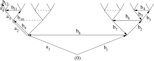
Figure 7: Two paths starting from the vertex 0 are drawn. The bonds of the two paths are indicated as $a_{1},a_{2},\ldots$ and $b_{1},b_{2},\ldots$, respectively. The two paths overlap each other in correspondence of the bonds $a_{2}=b_{9}$ and $a_{4}=b_{12}$. These bonds on the figure are slightly shifted for visual convenience.

5 Phase diagram of the random model

In the two following subsections we apply the mapping to study the phase diagram of the disordered model introduced in Sec. 2.2. Note that, as manifested in Fig. 3, the P-F and the P-AF transitions are completely asymmetric one another and since they can occur only for positive and negative values of $J_{\mathrm{1}}$, respectively, it will be sufficient to consider only the P-F and the P-SG transitions. Therefore, from now on we will study only the region with $J_{\mathrm{1}}\geq 0$ corresponding to Eqs. (7) and (20) that here we rewrite

$$t_{2}^{(\sigma)}((t_{1}^{(\sigma)})^{2}-2t_{1}^{(\sigma)})+1-2t_{1}^{(\sigma)}=0,\quad\sigma=\mathrm{F,SG}.$$ (25)

We observe that Eq. (25) (as well as Eq. (21)), with respect to $t_{1}^{(\sigma)}$, are quadratic and biquadratic under the transformations (30) and (33), respectively, so that we can solve this equation explicitly with respect to $t_{1}^{(\sigma)}$. This procedure turns out to be convenient for studying some asymptotes since we want to plot the critical lines on the plane $(T/J_{1},J_{2}/J_{1})$. Let us put

$$\kappa(x)\equiv\frac{1+x-\sqrt{1+x+x^{2}}}{x}.$$ (26)

In terms of $t_{1}^{(\sigma)}$, the solution of Eq. (25) for $t_{2}^{(\sigma)}$ can be expressed as

$$t_{1}^{(\sigma)}=\kappa(t_{2}^{(\sigma)}).$$ (27)

5.1 Triangular $\pm J$ model

For the triangular $\pm J$ model the randomness is given through Eqs. (5) and (6) which, plugged in the transformations (15) and (18), give respectively

$$\left\{\begin{array}[]{l}t_{1}^{(\mathrm{F})}=(2p_{\mathrm{1}}-1)t_{1},\\ t_{2}^{(\mathrm{F})}=(2p_{\mathrm{2}}-1)t_{2},\end{array}\right.$$ (30)

and

$$\left\{\begin{array}[]{l}t_{1}^{(\mathrm{SG})}=t_{1}^{2},\\ t_{2}^{(\mathrm{SG})}=t_{2}^{2}.\end{array}\right.$$ (33)

Note that in the last case there is no dependence on the values on $p_{\mathrm{1}}$ and $p_{\mathrm{2}}$, so that in the triangular $\pm J$ model model the P-SG transition is unique. Note also that Eqs. (30) are unchanged under the exchanges $p_{\mathrm{1}}\to 1-p_{\mathrm{1}}$ and $J_{\mathrm{1}}\to-J_{\mathrm{1}}$, and $p_{\mathrm{2}}\to 1-p_{\mathrm{2}}$ and $J_{\mathrm{2}}\to-J_{\mathrm{2}}$, respectively. Therefore, it will be sufficient to restrict ourself to the region

$$\left\{\begin{array}[]{l}p_{\mathrm{1}}\geq 0.5,\\ p_{\mathrm{2}}\geq 0.5.\end{array}\right.$$ (36)

From (27) the solution for the P-SG line (in terms of $t_{2}^{(\mathrm{SG})}$) is

$$\frac{T_{c}^{(\mathrm{SG})}(J_{\mathrm{2}})}{J_{\mathrm{1}}}=\left[\mathop{\rm\tanh^{-1}}\nolimits\left(\kappa(t_{2}^{(\mathrm{SG})})\right)^{1/2}\right]^{-1},$$ (37)

while the solution for the P-F lines (in terms of $t_{2}^{(\mathrm{F})}$) is

$$\frac{T_{c}^{(\mathrm{F})}(J_{\mathrm{2}})}{J_{\mathrm{1}}}=\left[\mathop{\rm\tanh^{-1}}\nolimits\left(\frac{\kappa(t_{2}^{(\mathrm{F})})}{2p_{\mathrm{1}}-1}\right)\right]^{-1}.$$ (38)

As an argument based on the high temperature expansion of the free energy suggests, we see in Fig. 8 that the presence of loops, tuned by fixing $J_{\mathrm{1}}$ and increasing the amplitude of the parameter $J_{\mathrm{2}}$, increases the spin glass critical temperature $T_{c}^{(\mathrm{SG})}$. In particular, the values of $T_{c}^{(\mathrm{SG})}$ for $J_{\mathrm{2}}\to 0$ and $J_{\mathrm{2}}\to\infty$ are given respectively by

$$\frac{T_{c}^{(\mathrm{SG})}(J_{\mathrm{2}}\to 0)}{J_{\mathrm{1}}}=\left[\mathop{\rm\tanh^{-1}}\nolimits\left(\frac{1}{\sqrt{2}}\right)\right]^{-1}=1.13459,$$ (39)

$$\frac{T_{c}^{(\mathrm{SG})}(J_{\mathrm{2}}\to\infty)}{J_{\mathrm{1}}}=\left[\mathop{\rm\tanh^{-1}}\nolimits\left(\sqrt{2-\sqrt{3}}\right)\right]^{-1}=1.74487.$$ (40)

As we shall see below, for values of $p_{\mathrm{1}}$ and $p_{\mathrm{2}}$ sufficiently high and far from $0.5$ and for $J_{\mathrm{2}}>0$, a similar behavior holds for the disordered ferromagnetic transition as well. Note however that unlike Eq. (37), for Eq. (38) exist regions without solution. Finally, observe that, for $J_{\mathrm{1}}$ finite, the asymptotic values of $T_{c}^{(\mathrm{SG})}$ or $T_{c}^{(\mathrm{F})}$ for $J_{\mathrm{2}}=0$ and $J_{\mathrm{2}}=+\infty$ correspond to the values of a pure Bethe lattice case and to a system with an infinitely strong loops effects, respectively. Note that in the latter case, if $J_{\mathrm{1}}\to 0$, $T_{c}^{(\mathrm{SG})}$ and $T_{c}^{(\mathrm{F})}$ also $\to 0$, the lattice being just an infinite set of non interacting dimers of spins: a gas of dimers. We point out that this last situation differs from the one in which $J_{2}\to\pm\infty$ and $J_{1}$ remains finite: an arbitrary small but non zero coupling $J_{1}$ make the structure with triangular loops non reducible to dimers.

5.1.1 The case $p_{\mathrm{1}}=p_{\mathrm{2}}$.

Here we discuss an analysis carried out for the simpler case $p\equiv p_{\mathrm{1}}=p_{\mathrm{2}}$. We have performed a study for the disordered P-F transition for several values of $p$. In Fig. 8 we report these lines. For $p=1$ one recovers the non random ferromagnetic transition (Fig. 3). In general for fixed parameters $J_{\mathrm{1}}$ and $J_{\mathrm{2}}$, as the value of $p$ is decreased from 1.00 toward 0.50, the critical temperature $T_{c}^{(\mathrm{F})}$ decreases continuously. For a fixed value of $p$, as the value of $J_{\mathrm{2}}$ increases the P-F lines reach a horizontal asymptote whose value can be obtained explicitly from Eq. (38)

$$\frac{T_{c}^{(\mathrm{F})}(J_{\mathrm{2}}\to+\infty)}{J_{\mathrm{1}}}=\left[\mathop{\rm\tanh^{-1}}\nolimits\left(\frac{\kappa(A)}{A}\right)\right]^{-1},$$ (41)

where $A=2p-1$. When $J_{2}$ decreases toward 0 from Eq. (38) we get

$$\frac{T_{c}^{(\mathrm{F})}(J_{\mathrm{2}}\to 0)}{J_{\mathrm{1}}}=\left[\mathop{\rm\tanh^{-1}}\nolimits\left(\frac{1}{2A}\right)\right]^{-1}.$$ (42)

Finally for negative values of $J_{2}$ the P-F lines reach a final point given by Eq. (38)

$$\frac{T_{c}^{(\mathrm{F})}(J_{\mathrm{2}}\to-\infty)}{J_{\mathrm{1}}}=\left[\mathop{\rm\tanh^{-1}}\nolimits\left(\frac{\kappa(-A)}{A}\right)\right]^{-1}.$$ (43)

Note that, for fixed $J_{1}$, Eq. (41) has no solution for values of $p\leq 0.6909$, whose asymptote corresponds to $T_{c}^{(\mathrm{F})}/J_{\mathrm{1}}=0$. Similarly, for fixed $J_{1}$ and for $J_{\mathrm{2}}\to-\infty$ Eq. (43) has solution only for the pure ferromagnetic case $p=1$. Note however that in both the cases the above temperatures $T_{c}^{(\mathrm{F})}$ are lower than $T_{c}^{(\mathrm{SG})}$ so that, according to Eq. (19), the actual phase in these regions is SG and the above $T_{c}^{(\mathrm{F})}$’s represent only unstable (not physically relevant) transitions.

By using Eq. (19), in the plane $(T/J_{\mathrm{1}},J_{\mathrm{2}}/J_{\mathrm{1}})$, as evident from Figs. 8 and 9, one finds the following scenario. Let us consider first the case $J_{\mathrm{2}}\geq 0$. For $p\geq 0.85\pm 0.01$ for any value of the parameters $J_{\mathrm{1}}$ and $J_{\mathrm{2}}$ the transition can be only P-F. For $p\in[0.81,0.85]\pm 0.01$ there is a range of values $J_{\mathrm{1}}$ and $J_{\mathrm{2}}$ where the stable transition is P-SG and a range where the stable transition is P-F. We note also that for $p\sim 0.81$ there can be more separated such ranges. Finally for $p<0.81\pm 0.01$ the transition can only be P-SG. Let us now consider the case $J_{\mathrm{2}}<0$. As is evident from Fig. 9, whereas for $J_{\mathrm{2}}/J_{\mathrm{1}}>-1$ for any value of $p$ the system may have both a P-F or a P-SG transition, for $J_{\mathrm{2}}/J_{\mathrm{1}}<-1$ the system has only a P-SG transition (similarly, for $J_{1}<0$ the P-AF transition may occur only if $J_{\mathrm{2}}/J_{\mathrm{1}}>1$). Recall that, under the restriction of Eq. (36), the averages of the couplings have the same sign of the parameters $J_{1}$ and $J_{2}$. For $p>0.5$, the two completely different scenarios between the two cases $J_{\mathrm{2}}>0$ and $J_{\mathrm{2}}<0$ reflect the difference of the average of the frustration over the triangles, positive in the former and negative in the latter case. By looking back at the transformations (30), we see that, concerning the disordered P-F transitions, the mapping consists in a simple renormalization of the couplings $J_{1}$ and $J_{2}$ so that the same argument used in Sec. 3 to describe the frustrated regions and, in particular, the dimers-triangles transition, applies again. On the other hand, unlike the non random case, for $J_{2}/J_{1}<-1$ there exists always a stable and unique P-SG transition, signaling the onset of overlaps orderings. It is interesting to observe that a picture in terms of non interacting dimers can be found even in the glassy phase in the limit $|J_{2}|\gg|J_{1}|$ with $J_{1}$ kept fixed. In such a limit in fact, the spins over a dimer must be exactly parallel or antiparallel, for $J_{x,y}^{(2)}>0$ or $J_{x,y}^{(2)}<0$, respectively, regardless of the values of the other couplings $J_{x,y}^{(1)}$, so that the average over the disorder of the local magnetization of any spin gives zero.

In Fig. 10 we report the detail of the phase diagram of the case $p=0.83$ providing even the neighborhood of the F-SG crossover.

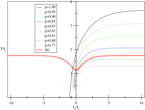
Figure 8: Critical lines of the disordered transition P-F for several values of $p\equiv p_{\mathrm{1}}=p_{\mathrm{2}}$ and the P-SG line. Note that, according to Eq. (19), for any given $p$, there is a unique stable upper critical line obtained by taking the convex construction as shown in Fig. 10.

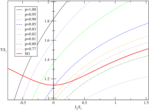
Figure 9: Enlargement of Fig. 8 around the SG line.

Figure 10: Phase diagram for the case $p_{\mathrm{1}}=p_{\mathrm{2}}=0.83$ in the neighborhood of the multicritical point P-F-SG. The line drawn between the SG and the F phase is the Nishimori line which, as is known, passes inside the F phase.

Finally, we point out that, as it must be, for any choice of $p$, the multicritical point F-P-SG belongs to the Nishimori line. This fact can be immediately checked by substituting $\tanh(\beta J)=2p-1$ into Eqs. (30) and (33).

5.1.2 The general case.

As shown in Fig. 11, for arbitrary values of the parameters $p_{\mathrm{1}}$ and $p_{\mathrm{2}}$ the scenario of the possible transition lines becomes of course reacher. In the region $J_{\mathrm{2}}\geq 0$ we do not observe relevant qualitative differences with respect to the case $p_{\mathrm{1}}=p_{\mathrm{2}}$. We see that in general, for any fixed value of $p_{\mathrm{1}}$, by varying $p_{\mathrm{2}}$ one obtains a family of non intersecting critical lines margins at $J_{\mathrm{2}}=0$ (as given by Eq. (42)) and whose $T_{c}$ in general becomes lower as $p_{\mathrm{2}}$ decreases. For fixed values of $p_{\mathrm{1}}$ and $p_{\mathrm{2}}$, as the value of $J_{\mathrm{2}}$ increases, the P-F lines reach a horizontal asymptote whose value can be explicitly calculate from Eq. (38)

$$\frac{T_{c}^{(\mathrm{F})}(J_{\mathrm{2}}\to+\infty)}{J_{\mathrm{1}}}=\left[\mathop{\rm\tanh^{-1}}\nolimits\left(\frac{\kappa(B)}{A}\right)\right]^{-1},$$ (44)

where $A=2p_{\mathrm{1}}-1$ and $B=2p_{\mathrm{2}}-1$. From Fig. 11 we observe also that two critical lines having two different values of $p_{\mathrm{1}}$, in general, may intersect each other. In the region $J_{\mathrm{2}}<0$ we observe that if $p_{\mathrm{1}}$ is sufficiently high, (starting from $p_{\mathrm{1}}\sim 0.85$) and $p_{\mathrm{2}}\neq p_{\mathrm{1}}$, as $J_{\mathrm{2}}$ decreases, the transition lines can have an inversion and reach another horizontal asymptote whose value is given by

$$\frac{T_{c}^{(\mathrm{F})}(J_{\mathrm{2}}\to-\infty)}{J_{\mathrm{1}}}=\left[\mathop{\rm\tanh^{-1}}\nolimits\left(\frac{\kappa(-B)}{A}\right)\right]^{-1}.$$ (45)

Note that the temperatures given by this equation are lower than the ones obtained in the opposite limit $J_{\mathrm{2}}\to+\infty$. Note also that Eqs. (44) and (45) have no solution for values of $p_{\mathrm{1}}$ and $p_{\mathrm{2}}$ such that $A^{2}B-2AB-2A+1=0$ and $A^{2}B-2AB+2A+1=0$, respectively. But analogously to the case previously seen ($p_{\mathrm{1}}=p_{\mathrm{2}}$), as evident from Fig. 11, these regions of non existence occur only for values of $p_{\mathrm{1}}$ and $p_{\mathrm{2}}$ quite lower than the threshold at which the only stable transition is P-SG.

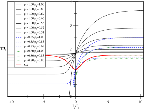
Figure 11: Critical lines of the disordered transition P-F for several values of $p_{\mathrm{1}}$ and $p_{\mathrm{2}}$ and the P-SG line.

6 Conclusions

The phase diagram of a competitive Ising model defined over the triangular Husimi tree has been analyzed, both in the non random and the random version (spin glass model). First, we have analyzed the non random case providing, in particular, an interesting physical characterization of the ground states in the frustrated regions in terms of a zero temperature phase transition between an ordered or antiordered state of connected triangles (F or AF) and a gas of non interacting two state dimers (also called a spin liquid in the literature). A natural question is whether or not this zero temperature phase transition represents the zero temperature boundary of a finite temperature phase transition. Second, we have introduced the disorder and studied the upper phase diagram and the corresponding critical behavior of the random case which, in particular, gives an affirmative answer to the above question. Our method relies on a recently proposed mapping valid for a wide family of graphs turning out to be infinite dimensional in a broad sense, as happens (but not only) in generalized tree-like graphs and in suitable structures where an infinite number of closed paths per vertex is also allowed. This second class includes, in particular, generalized Bethe lattices and Husimi trees, i.e., graphs over which non random models are exactly solvable. The mapping maps the spin glass model onto the corresponding non random one. For the two couplings $J_{\mathrm{1}}$ and $J_{\mathrm{2}}$ we have chosen the disorder giving rise to the triangular $\pm J$ model. We can observe directly the role of the explicit frustration induced by the presence of the loops tuned by the amplitude and the sign of the parameter-coupling $J_{\mathrm{2}}$. As expected from an argument based on high temperature expansion and on frustration, the spin glass critical temperature is a nondecreasing function of $|J_{\mathrm{2}}|$, whereas the disordered ferromagnetic critical temperatures is a nondecreasing function of $J_{\mathrm{2}}$. We observe the following scenario. In the non frustrated regions (that is the sectors I and III of the phase diagrams), in the spin glass model we find an “ordinary” competition (like in the Sherrington Kirkpatrick model) between a P-SG and a P-F or P-AF transitions, in which the parameters $J_{1}$ and $J_{2}$ are simply renormalized by the mapping and the spin glass transition signals the onset of spin overlaps. In the frustrated regions instead (sectors II and IV of the phase diagrams), we find a new feature; in fact, even for $|J_{2}|>|J_{1}|$, there exists always a phase transition which turns out to be a P-SG phase transition (the red line in the Figs. 8-11), whose glassy phase consists again of a gas of non interacting two state dimers.

The analytical study carried out here concerns a non trivial model defined over a structure where loops are important. Other more complex and variegated cases, such as other Ising models with more than two couplings and Potts models, could be similarly analyzed.

Even if, as stressed in Sec. I, in the Husimi tree, we do not have the existence of $\varphi_{I}$, the density free energy in the thermodynamic limit, which is a necessary condition for the mapping, we think nevertheless that the application of the mapping also in this case provides important information of the random model. We stress in fact that in the mapping no ad hoc approximation is introduced.

Appendix A

A comment is in order concerning the model considered in the Ref. [13] (and partially in [14, 15]), which is defined on the finite Husimi tree of Fig. 2, and the model given in Sec. 2.1, which is defined on the corresponding infinite Husimi tree (which can be seen as a Bethe lattice with loops).

Whereas in the infinite Husimi tree one has to solve the model with the Hamiltonian (1) for vertices far from the boundary, and this is done by considering in all the calculation the lattice as infinite from the very beginning, in the finite Husimi tree one has to take into account also the boundary in the finite lattice and to perform the thermodynamic limit in the proper manner by calculating the correlation functions only from the density free energy after the thermodynamic limit has been taken. The relations between infinite and finite Husimi trees are on the same level of those between Bethe lattices and Cayley trees. It turns out that the physics, and in particular the free energy, described by these two versions of models is quite different [40, 41, 42]. Nevertheless, the equations defining the effective fields for the central spin used in both the approaches are the same implying that also the fixed points, and then the equations for the critical surfaces and the magnetization of the central spin, are the same. We show this now by deriving the equations for the infinite Husimi tree following the so called Baxter approach [1], subsequently adapted to generalized Bethe lattices by many authors (see [10] and references therein) and to Husimi trees by [11].

Let us indicate with $Z_{n}(\sigma_{0})$ the conditional partition function of the root spin $\sigma_{0}$ (see Fig. 2) for the $n$-th generation graph; that is the graph of Fig. 2 having $n$ shells completed, having $|S_{n}|$ vertices, plus an external circular annulus $C_{n}$, having the latter a number $|C_{n}|$ of vertices such that $|S_{n}|/|C_{n}|\to 0$ as $n\to\infty$. We have

$$Z_{n}=\sum_{\sigma_{0}}Z_{n}(\sigma_{0}),$$ (46)

where $Z_{n}$ is the full partition function of the $n$-th generation graph. By looking at Fig. 2, it is easy to see that the conditional partition function $Z_{n+1}(\sigma_{0})$ of the root spin at the $n+1$-th generation graph is related to $Z_{n}(\sigma_{0})$ through

$$Z_{n+1}(\sigma_{0}) = \sum_{\sigma_{1},\sigma_{2}}e^{-B\sigma_{0}+k_{1}\sigma_{0}(\sigma_{1}+\sigma_{2})+k_{2}\sigma_{1}\sigma_{2}}Z_{n}(\sigma_{1})Z_{n}(\sigma_{2}),$$ (47)

where $B=\beta h$, $k_{1}=\beta J_{1}$, $k_{2}=\beta J_{2}$, and $\sigma_{1}$ and $\sigma_{2}$ are the two Ising variables located at the vertices 1 and 2 respectively in Fig. 2. It is convenient to introduce the effective field $h_{n}$:

$$e^{2h_{n}}=\frac{Z_{n}(-)}{Z_{n}(+)}.$$ (48)

Performing the sums over $\sigma_{1}$ and $\sigma_{2}$ in Eq. (47) both for $\sigma_{0}=+$ and $\sigma_{0}=-$, and using the definition (48) we arrive at the following closed recursive equation for the effective field

$$e^{2h_{n+1}}=e^{2B}\frac{e^{-2k_{1}+k_{2}}+2e^{-2k_{2}+2h_{n}}+e^{2k_{1}+k_{2}+4h_{n}}}{e^{2k_{1}+k_{2}}+2e^{-2k_{2}+2h_{n}}+e^{-2k_{1}+k_{2}+4h_{n}}}.$$ (49)

All the possible phase transitions (except the modulated ones) of the uniform model can be studied analyzing the fixed points $h^{*}$ of the above equation:

$$e^{2h^{*}}=e^{2B}\frac{e^{-2k_{1}+k_{2}}+2e^{-2k_{2}+2h^{*}}+e^{2k_{1}+k_{2}+4h^{*}}}{e^{2k_{1}+k_{2}}+2e^{-2k_{2}+2h^{*}}+e^{-2k_{1}+k_{2}+4h^{*}}}.$$ (50)

Of course one can use Eq. (50) to write the recursive equation for the magnetization for the root spin $\sigma_{0}$. If one is interested in studying the individual magnetizations of further spins as for the spins $\sigma_{1}$ and $\sigma_{2}$, then one has to write the recursive equations for the conditional partition function $Z_{n+1}(\sigma_{0},\sigma_{1},\sigma_{2})$ in terms of weighted sums over $\sigma_{1,1},\ldots\sigma_{2,2}$ of the conditional partition functions $Z_{n}(\sigma_{1},\sigma_{1,1},\sigma_{1,2})$ and $Z_{n}(\sigma_{2},\sigma_{2,1},\sigma_{2,2})$ (see Fig. 2) and defining the corresponding effective fields. In this way one can study possible modulated phases as done for example in [10] for generalized Bethe lattices involving second and third-nearest neighbor interactions.

In the model considered in this paper, the base spin $\sigma_{0}$ is attached to one single triangle (see Fig. 2). However one could be interested in studying cases in which the root spin has to be attached to more, say $q$, triangles. It is immediate to recognize that in this case instead of Eq. (50) one has

$$e^{2h^{*}}=e^{2B}\left[\frac{e^{-2k_{1}+k_{2}}+2e^{-2k_{2}+2h^{*}}+e^{2k_{1}+k_{2}+4h^{*}}}{e^{2k_{1}+k_{2}}+2e^{-2k_{2}+2h^{*}}+e^{-2k_{1}+k_{2}+4h^{*}}}\right]^{q}.$$

The model considered in this paper corresponds to the case $q=1$ of Eq. (50) which was also derived in [13] for the finite Husimi tree. As already mentioned, despite the physics for the infinite and finite Husimi trees be different, the equations for the effective fields are the same, or in other words, the physics of the “central” spins, far from the boundary, are the same. Therefore we can, in particular, use the analysis of the Ref. [13] for the phase transitions consisting in the study of the solutions of Eq. (50) and their stability leading to the Eqs. (7) and (8).

References

References

- [1] R. J. Baxter, Exact Solved Models in Statistical Mechanics (Academic Press, London, 1982). See also Sec. 2 of the Ref. [33].
- [2] S.N. Dorogovtsev, J.F.F. Mendes, Evolution of Networks (University Press: Oxford, 2003).
- [3] R. Pastor-Satorras, A. Vespignani, Evolution and Structure of the Internet (University Press: Cambridge) (2004).
- [4] R. Albert, A.L. Barab´asi, Rev. Mod. Phys. 74 47 (2002).
- [5] S.N. Dorogovtsev, J.F.F. Mendes, Adv. Phys. 51 1079 (2002).
- [6] S.N. Dorogovtsev, A.V. Goltsev, J.F.F. Mendes, 2002 Phys. Rev. E 66 016104-1 (2002).
- [7] M. Leone, A. Va´zquez, A. Vespignani, R. Zecchina, Eur. Phys. J. B 28 191 (2002).
- [8] R. Lyons, Comm. Math. Phys. 125 337-353 (1989).
- [9] R. Lyons, Jour. Math. Phys. 41, 3 : 1099-1126 (2000).
- [10] C.R. da Silva, S. Coutinho, Phys. Rev. B,34, 7975-7985 (1986).
- [11] J. Monroe, J. Stat. Phys. 65 (1991) 255; J. Stat. Phys. 67 (1992) 1185; Physica A 256 (1998) 217; Phys. Rev. E 64 (2001) 016126; Phys. Rev. E 65 (2002) 026109.
- [12] N.N. Ganikhodjaev, C.H. Pah, M.R.B. Wahiddin, J.Phys. A: Math. Gen. 36, 4283-4289 (2003).
- [13] N.N. Ganikhodjaev, C.H. Pah, M.R.B. Wahiddin, J. Math. Phys. 45, 3645 (2004).
- [14] F. Mukhamedov, U. Rozikov, J. Stat. Phys. 114, 825 (2004).
- [15] F. Mukhamedov, U. Rozikov, J. Stat. Phys. 119, 427 (2005).
- [16] N. Ganikhodjaev, F. Mukhamedov, J. F.F. Mendes J. Stat. Mech. P08012 (2006).
- [17] F. Mukhamedov, U. Rozikov, math-ph/0510022.
- [18] C. Domb, Adv. Phys. 9, 145 (1960).
- [19] S.N. Dorogovtsev, A.V. Goltsev, J.F.F. Mendes, Critical phenomena in complex networks, arXiv:0705.0010v2.
- [20] J. Vannimenus, Z.Phys. B 43, 141–148 (1981). We point out that, unlike the simpler models faced in the Refs. [12]-[16], the approaches used for the models considered in Refs. [20]-[24] were analytical only partially and, in partcular, a general and rigorous picture of the phase diagrams was lacking.
- [21] T. Horiguchi and T. Morita, J. Phys. A 16, 3611 (1983).
- [22] M. Mariz, C. Tsalis, A.L. Albuquerque, J. Stat. Phys. 40, 577-592 (1985).
- [23] C.S.O.Yokoi, M.J. de Oliveira, S.R. Salinas, Phys. Rev. Lett. 54, 163–166 (1985).
- [24] M.H.R. Tragtenberg, C.S.O. Yokoi, Phys. Rev. E 52, 2187-2197 (1995).
- [25] R.J. Elliott, Phys. Rev.,124, 340–345 (1961).
- [26] P. Bak, J.von Boehm, Phys. Rev. B, 21 5297–5308 (1980).
- [27] G. Toulouse, Comm. on Phys. 2 115 (1977).
- [28] M. Mezard, G. Parisi, M.A. Virasoro, 1987 Spin Glass Theory and Beyond (Singapore: World Scientific)
- [29] M. Ostilli, J. Stat. Mech. P10004 (2006).
- [30] M. Ostilli, J. Stat. Mech. P10005 (2006).
- [31] M. Ostilli, arXiv:0706.1949. To appear in J. Stat. Mech..
- [32] R. Mélin and S. Peysson, Eur. Phys. J. B 14 169 (2000).
- [33] M. Mezard, G. Parisi, Eur. Phys. J. B 20, 217-233 (2001).
- [34] C. N. Likos, Phys. Rev. E 55 (1997); see also references therein.
- [35] G. Bianconi, M. Marsili, J. Stat. Mech. P06005 (2005).
- [36] A. Montanari, T. Rizzo, J. Stat. Mech. P10011 (2005).
- [37] G. Parisi and F. Slanina, J. Stat. Mech. L02003 (2006).
- [38] E. Marinari and G. Semerjian, J. Stat. Mech. P06019 (2006).
- [39] M. Chertkov and V. Y Chernyak, J. Stat. Mech. P06009 (2006).
- [40] T. P. Eggarter Phys. Rev. B, 9, 2989 (1973).
- [41] E. Mller-Hartman and J. Zittartz, Phys. Rev. Lett. 33, 893 (1974).
- [42] F. Peruggi, J. Phys. A 16, L713 (1983).
- [43] Due to this similarity with a glassy phase, we could alternatively use the expression “liquid of dimers” instead of “gas of dimers” for this phase. Of course such a distinction for our model is just a lexical fact.
- [44] In the Ref. [29] was claimed that the probability for the overlap has to go zero for . Of course such a relation has to be satisfied if is a probability. The above statement remains sensible but only heuristic. In fact, more precisely, it is necessary to define the probability for two finite paths of lenght and to overlap times, , and to analyze its behavior for . It is possible then to show rigorously that the uniform bound , with and two positive constant, is a sufficient condition for the mapping to become exact [31]. Note that, in general, such a bound does not guarantee the existence of an asymptotic probability . However, in the case of Bethe lattices or Husimi trees (and in many random graphs) one has also the existence of , so that the sufficient condition can be directly verified looking at the distribution .