Synchronization in weighted scale free networks
with degree-degree correlation

Abstract

We study synchronization phenomena in scale-free networks of asymmetrically coupled dynamical systems featuring degree-degree correlation in the topology of the connection wiring. We show that when the interaction is dominant from the high-degree to the low-degree (from the low-degree to the high degree) nodes, synchronization is enhanced for assortative (disassortative) degree-degree correlations.

Keywords: Complex Network, Synchronization. 89.75.-k,05.45Xt

Recent years have witnessed increasing interest in the study of the structure of complex networks. Networks are present ubiquitously in the real world, including biological systems, genetic chains, social relationships and artificial and engineering architectures [2]. A main quantity that characterizes the structure and dynamics of those networks is the so called degree distribution $P(k)$, the probability that a randomly chosen node within the network has degree $k$, i.e. there are $k$ connections incident in it. In most cases, this distribution has been found to obey a power law $P(k)\sim k^{-\gamma}$, with $\gamma$ usually ranging between 2 and 3. The slow decay of the power-law distribution, when the exponent is within the observed values, is responsible for the presence of few high-degree nodes, usually termed as hubs, which play a leading role in characterizing the network dynamical behavior. Thus the network structure (termed in this case as scale free) displays high heterogeneity, with the presence of a few high-degree vertices and many low-degree ones.

Beyond the specific interest in the study of the main topological properties of such networks, there is an ongoing research effort to understand how these statistical features affect the dynamical processes taking place over them, as e.g. epidemic spreading [24, 3, 19], communication models [23, 10, 11, 1] and spin systems [8, 9, 14]. Among these, a relevant phenomenon is the emergence of collective synchronized motion. This corresponds to the case of several dynamical systems, starting from different initial conditions appropriately coupled with a network topology, stabilizing in a common evolution.

In this framework, we consider the case of networks of coupled identical systems, that can be conveniently described by the following set of ordinary differential equations:

$$\frac{dx_{i}}{dt}=f(x_{i})-\sigma\sum_{j=1}^{N}{\mathcal{L}}_{ij}h(x_{j}),\qquad i=1,2,...N,$$ (1)

where ${x}_{i}\in{\mathbb{R}}^{m}$ is the $m$-dimensional vector describing the state of the $i^{\text{th}}$ node, ${f}({x_{i}}):{\mathbb{R}}^{m}\to{\mathbb{R}}^{m}$ governs the dynamics of the $i^{\text{th}}$ node, ${h}({x}):{\mathbb{R}}^{m}\to{\mathbb{R}}^{m}$ is a vectorial output function, $\sigma$ is a parameter ruling the coupling strength, and $N$ is the number of nodes of the network. The topological information on the graph is contained in the connection matrix $\mathcal{L}$. Specifically $\mathcal{L}=\{\mathcal{L}_{ij}\}$ is defined as follows:

$$\mathcal{L}_{ij}=-\mathcal{A}_{ij}\mathcal{W}_{ij},\quad i\neq j$$

$$\mathcal{L}_{ij}=\sum_{j}\mathcal{A}_{ij}\mathcal{W}_{ij},\quad i=j,$$ (2)

where $\mathcal{A}$ is the irreducible adjacency matrix associated to the network topology, that is $\mathcal{A}_{ij}=\mathcal{A}_{ji}=1$, if there is a connection between $i$ and $j$, $0$ otherwise. $\mathcal{W}$ is a positive definite matrix containing the information about the weights over the network connections, with $\mathcal{W}_{ij}$ giving a measure of the strength of the interaction from node $i$ to node $j$.

Note that (1) and (2) encompass a general and large class of networks, allowing for non-linearity in the functions $f$ and $h$ and leaving complete freedom for the choice of the weights over the network connections. The only constraint is represented by the condition $\mathcal{L}_{ii}=-\sum_{j\neq i}\mathcal{L}_{ij}$, which is necessary in order to guarantee that the connection matrix $\mathcal{L}$ is zero row-sum.

When the connection matrix $\mathcal{L}$ is symmetric, the network propensity to synchronization (the so-called network synchronizability) can be studied rigorously by means of the Master Stability Function (MSF) approach [25]. Namely, the MSF assesses the necessary conditions for the transverse stability of the synchronization manifold $x_{1}=x_{2}=...=x_{N}=x_{s}$, whose existence as an invariant set for the system in (1) is warranted by the zero row-sum property of $\mathcal{L}$.

Indeed, let $\delta{x}_{i}(t)={x}_{i}(t)-{x}_{s}(t)$ be the deviation of the $i^{\text{th}}$ vector state from the synchronization manifold, and consider the $m\times N$ column vectors $\mathbf{X}=({x}_{1},{x}_{2},\ldots,{x}_{N})^{T}$ and $\delta\mathbf{X}=(\delta{x}_{1},\ldots,\delta{x}_{N})^{T}$.

Then, one has

$$\delta\dot{\mathbf{X}} = \left[{\mathbb{I}}_{N}\otimes{J}{f}({x}_{s})-\sigma{\cal L}\otimes{J}{h}({x}_{s})\right]\delta\mathbf{X},$$ (3)

where $Jf$ and $Jh$ represent the Jacobian operators of the system dynamics and coupling. Following [25], Eq. (3) can be block-diagonalized in the form:

$$\frac{d\eta_{i}}{dt}=[Jf(x_{s})-\sigma\lambda_{j}Jh(x_{s})]\eta_{i},\quad j=1,2,...,N,$$ (4)

where $\{\lambda_{j}\}=\{\lambda_{j}^{r}+i\lambda_{j}^{i}\}$ is the set of eigenvalues of the coupling matrix $\mathcal{L}$ (supposed diagonalizable), ordered in such a way that $\lambda_{1}^{r}\leq\lambda_{2}^{r}...\leq\lambda_{N}^{r}$. Notice that $\lambda_{1}$ is identically equal to $0$, due to the zero row-sum condition, and the corresponding eigenvector is the unitary vector pointing in a direction parallel to the synchronization manifold. Therefore, the modes of the system along this direction are not relevant, since one has only to care for whether the system will synchronize or not, independent of where this happens in phase space. Thus, the stability of the synchronization manifold should be checked with respect to perturbations lying in phase space along directions orthogonal to it (those associated to the eigenvalues $\lambda_{2},...,\lambda_{N}$).

In order to study the stability of the synchronization manifold as a function of the eigenvalues of the matrix $\mathcal{L}$, one introduces the following parametric equation in $\alpha$:

$$\frac{d\eta}{dt}=[Jf(x_{s})-\alpha Jh(x_{s})]\eta,$$ (5)

where $\alpha$ takes the place of $\sigma\lambda_{j}$ in eq. (4). Note that $Jf$ and $Jh$ do not depend on the network topology. Moreover, for simplicity, one can rewrite (5) as:

$$\frac{d\eta}{dt}=K(\alpha)\eta,$$ (6)

where $K(\alpha)$ is the evolution kernel, as a function of $\alpha$. The MSF associates to each value of the parameter $\alpha$ in the complex plane, the maximum (conditional) Lyapunov exponent of the system calculated along trajectories of (6).

Now, in most cases (i.e. for most of the forms of the functions $f$ and $h$), the MSF is negative in a bounded region of the complex plane (termed as the stability region $\mathcal{S}$). The immediate consequence of this is that the network synchronizability is related to the distribution of the eigenvalues of the coupling matrix $\mathcal{L}$. Specifically, the stability of the synchronization manifold requires as a necessary condition that all the $\sigma\lambda_{j}$, $j=2,...,N$ belong to $\mathcal{S}$.

As proposed in [12], a sufficient condition to verify the above requirement is checking that the rectangle of the complex plane, $\mathcal{R}$: $[\sigma\lambda_{2}^{r},\sigma\lambda_{N}^{r}]\times[\sigma\min_{j}\lambda_{j}^{i},\sigma\max_{j}\lambda_{j}^{i}]$ is fully contained in $\mathcal{S}$ (observe also that the spectrum of $\mathcal{L}$ is symmetric with respect to the real axis and thus $M=\max_{j}\lambda_{j}^{i}=-\min_{j}\lambda_{j}^{i}$). Moreover this condition can be simplified with respect to different forms of the functions $f$ and $h$ into the general requirement that both the eigenratio defined as $R=\lambda_{N}^{r}/\lambda_{2}^{r}$ and $M$, the maximum imaginary part of the spectrum of $\mathcal{L}$, are as small as possible. In so doing, different network topologies become directly comparable in terms of their synchronizability, by simply looking at the indices $R$ and $M$.

Moreover, we wish to emphasize that there is no need for introducing an ordering between the two parameters $R$ and $M$, defined above; specifically, when they are both reduced, this leads to the general result that the range of values of $\sigma$, say $I_{\sigma}$, for which $\mathcal{R}$ is contained in $\mathcal{S}$ (and therefore the network synchronizability) increases. Note that this result is independent from the specific forms of $f$ and $h$, i.e. of the particular MSF considered.

It is worth noting that the block-diagonalization in (4) can be properly applied only to the case of symmetric and asymmetric diagonalizable matrices (in the particular case of a real spectrum, as e.g. when $\mathcal{L}$ is symmetric, we obtain the following simple relationship: the lower is $R$, the larger is the interval $I_{\sigma}$). Moreover, as explained in [21, 26], the same definition of network synchronizability (in terms of both $R$ and $M$) can be extended also to the case of non-diagonalizable matrices (see e.g. [15, 16, 4, 12]), when the condition is satisfied that the network embeds at least an oriented spanning tree. The case of generic directed networks has been studied in [5].

Thus in what follows we shall seek to characterize how the structural properties of complex networks, in terms of both the forms of the adjacency matrix $\mathcal{A}$ and the weights matrix $\mathcal{W}$, may affect (and eventually improve or hinder) their synchronizability.

The first contribution in this sense was provided in [22], where unweighed scale free networks were compared in terms of their synchronizability as varying the degree distribution exponent $\gamma$.

Note that in the case of unweighed topologies, $\mathcal{W}$ is assumed to be the unitary matrix and thus $\mathcal{L}$ can be simply expressed as $\mathcal{L}_{ij}=-\mathcal{A}_{ij}$ for $i\neq j$ and $\mathcal{L}_{ii}=\sum_{j}\mathcal{A}_{ij}$, $i=1,2,...,N$.

It can be shown that as the exponent $\gamma$ is increased, the network topology becomes more homogeneous and the average distance within pairs of connected nodes along the geodesic increases. For instance, real-world networks are characterized by low values of $\gamma$ in that they are affected by high heterogeneity in the degree distribution and low distances between pairs of connected sites (the so-called small-world effect).

Thus one would expect such networks to be characterized by high synchronizability, in order also to justify their onset in nature as being the result of a self-organized process. Instead, the analysis in [22] showed that these are typically characterized by lower synchronizability than their homogeneous counterparts, giving rise to an unexpected phenomenon, which is termed in the literature [16] as the paradox of heterogeneity.

This first result was overturned in [15] where an appropriate choice of the weights was considered over the network links of the form:

$$\mathcal{W}_{ij}={k_{i}}^{-\beta},\quad i\neq j,$$ (7)

where $k_{i}$ is the degree of node $i$, i.e. $k_{i}=\sum_{j}{\mathcal{A}_{ij}}$ and $\beta$ is a variable parameter.

Now, it is worth noting that in the real world, weights associated to the network links depend on an huge amount of variables; furthermore they are typically also variable in time. Thus, trying to estimate the effects of such a complex behavior, may be a difficult task. On the other hand, the approach proposed in [15] is very convenient in that it is aimed at evaluating the effects of variable weights, depending essentially on some network topological features. Namely, by varying $\beta$, it is possible to tune the strength of the coupling among the network nodes according to their degree: $\beta=0$ corresponds to the case of unweighed topologies, positive (negative) values of $\beta$ indicate that the strengths of the couplings acting on each vertex decreases (increases) with its degree. In [15] it was shown that the network synchronizability is optimized at $\beta=1$, whatever the form of the degree distribution. Specifically, it was claimed that in this optimal regime, the eigenratio $\lambda_{N}/\lambda_{2}$ is independent from the networks topological properties, other than the average degree (note that for a coupling of the form in (7), the parameter $M=0$ [15]).

The case of $\beta=1$ is of particular relevance also in another aspect. In fact, in such a case, $\mathcal{L}_{ii}=1\quad\forall i$ and $\sum_{j\neq i}\mathcal{L}_{ij}=-1\quad\forall i$. Gerschgorin circle theorem [12] states that the set of the eigenvalues $\{\lambda_{j}=\lambda_{j}^{r}+j\lambda_{j}^{i}\}$, belongs to the union of the circles (${\mathcal{C}}_{i}$) centered on the main diagonal values of $\mathcal{L}$ in the complex plane and with radius equal to the sum of the absolute values of the other elements in the corresponding rows, $(\{\lambda_{i}\}\subset\bigcap_{i}{\mathcal{C}_{i}[\mathcal{L}_{ii},\sum_{j\neq i}|\mathcal{L}_{ij}|]})$. Thus in the case of $\beta=1$, all the $\mathcal{C}_{i}$ coincide with the circle of radius $1$, centered at 1 on the real axis, inside which are constrained to lie all the $\lambda_{j}$, $\quad j=1,2,...,N$ [4]. Note that from this condition, we can draw the two following ones: (i) $0=\lambda_{1}^{r}\leq\lambda_{2}^{r}\leq...\leq\lambda_{N}^{r}\leq 2$, (ii) $\lambda_{j}^{i}\in[-1,1]$, $j=1,2,...,N$.

It is worth noticing here that for any given choice of the weights over the network connections $\mathcal{W}_{ij}$, the same requirements as above are satisfied by replacing (2) with

$$\mathcal{L}_{ij}=\frac{-\mathcal{A}_{ij}\mathcal{W}_{ij}}{\sum_{k}{\mathcal{A}_{ik}\mathcal{W}_{ik}}},\quad i\neq j$$

$$\mathcal{L}_{ij}=1,\quad i=j.$$ (8)

We wish to emphasize that this can be convenient in comparing networks characterized by different topological features in terms of their synchronizability. In fact, although the condition on the minimization of $\lambda_{N}/\lambda_{2}$ corresponds to an increase of the interval of the values of $\sigma$ for which the synchronization manifold is stable, it does not give any information about the values of $\sigma$ themselves. One possible consequence of this could be e.g., that although a network is more synchronizable than an other (in terms of their respective eigenratios), it experiences synchronization only for higher values of the coupling $\sigma$. Nonetheless this problem can be overcome by considering an appropriate coupling as in (8), which guarantees that $\lambda_{2}$ is lower-bounded by $0$ and $\lambda_{N}$ is upper-bounded by $2$ and thus ensures the spectra we are evaluating are characterized by the same scale.

By following this approach, in [4] it was shown that an even better result in terms of network synchronizability may be achieved by taking weights proportional to a specific topological quantity known as load [10] or betweenness centrality [17]. At the same time in [12], a particularly suitable way was proposed of choosing the weights over the network connections, according to the presence of a given ordering among the network nodes. Specifically the network nodes were ordered according to a given scalar property, say $p$, in such a way, i.e. that $i\leq j$ if $p(i)\leq p(j)$. Then the following general way of choosing the weights was proposed:

$$\mathcal{W}_{ij}=\frac{Q_{ij}}{\sum_{k}\mathcal{A}_{ik}Q_{ik}},$$ (9)

where $Q_{ij}=\frac{1-q}{2}$ ($Q_{ij}=\frac{1+q}{2}$) if $i<j$ ($i>j$), with $-1<q<1$ being a parameter governing the coupling asymmetry within the network. Note that, by varying $q$, it is possible to study the effects of variable asymmetric weights over the network edges. Specifically, in what follows we will consider a very natural way of choosing the weights based on a degree ordering (also termed as age ordering in [12]), i.e. such that $p(i)=k_{i}$. Namely, $q=0$ corresponds to the case of symmetric coupling, which is equivalent to the choice of $\beta=1$ in eq. (7). The limit of $q\rightarrow 1$ ($q\rightarrow-1$) corresponds to the case of a direct network in which only the connections from high-degree to low-degree vertices (from low-degree to high-degree) are present. Under this condition, it was shown in [12], that in the case of scale-free networks, synchronizability can be improved for decreasing values of $q$, i.e. when the strength of the coupling is dominating in the direction from the high-degree to the low-degree vertices.

Sofar, we have considered the effects of varying the weights over the network connections on the network synchronizability (in terms of the matrix $\mathcal{W}$), while the network topology (in terms of the matrix $\mathcal{A}$) has been considered as fixed. Nonetheless, it was shown in [22, 6], that even in the case of unweighed topologies, synchronizability may be strongly affected by varying some particular network topological properties.

The most important one is, as already stated before, the degree distribution, which affects in a non-negligible way almost all the dynamical processes taking place over networks [2]. On the other hand, many important properties have been discovered to characterize in more detail the network structure, other than the degree distribution. These are mostly due to particular forms of correlation or mixing among the network vertices [20].

One form of mixing is the correlation among pairs of linked nodes according to some properties at the nodes. A very simple case is degree correlation [18], in which vertices choose their neighbors according to their respective degrees. Non-trivial forms of degree correlation have been experimentally detected in many real-world networks, with social networks being typically characterized by assortative mixing (which is the case when vertices are more likely to connect to other vertices with approximately the same degree) and technological and biological networks, by disassortative mixing (that takes place when connections are more frequent between vertices of different degrees). In [18] this property has been conveniently measured by means of a single normalized index, the Pearson statistic $r$ defined as follows:

$$r={1\over{\sigma^{2}_{q}}}{\sum_{k,k^{\prime}}kk^{\prime}(e_{kk^{\prime}}-q_{k}q_{k^{\prime}})},$$ (10)

where $q_{k}$ is the probability that a randomly chosen edge is connected to a node having degree $k$; $\sigma_{q}$ is the standard deviation of the distribution $q_{k}$ and $e_{kk^{\prime}}$ represents the probability that two vertices at the endpoints of a generic edge have degrees $k$ and $k^{\prime}$ respectively. Positive values of $r$ indicate assortative mixing, while negative values characterize disassortative networks.

In [6] a strategy was used, similar to the one presented in [18], which allows to vary the degree correlation (in terms of variable values of $r$), while keeping fixed the degree distribution and it was shown that disassortative mixing, i.e. the tendency of high-degree nodes to establish connections with low-degree ones (and viceversa), is indeed a desirable network property in terms of its synchronizability. The same effect was checked in [7] to be persistent under a normalized form of the weighing as that proposed in [15], with $\beta=1$.

Here, we shall seek to characterize how the combination of the effects of variable degree correlation in terms of the structural configuration of the network, and variable asymmetry over the network weights may indeed affect the network synchronizability.

In order to construct networks, characterized by a given degree distribution (in terms of the exponent $\gamma$), we consider the network building model proposed in [13], which is commonly termed as the configuration model. Specifically this consists in the following steps:

1. Start from a given form of the degree distribution $P(k)$.

2. Assign to each of $N$ vertices a target degree $k>k_{min}$ drawn from the distribution $P(k)$.

3. Randomly create connections between pairs of vertices, avoiding multiple and self-connections, until all vertices have reached their target degree.

Then in order to reproduce a desired level of degree correlation, following [20], we propose exchanges of links between pairs of connected nodes, until the desired value of the observable $r$ is reached.

In what follows we have evaluated the effects on the network synchronizability of both variable values of $r$ and $q$. The main results are shown in Figs. 1 and 2, for scale free networks with degree distribution exponent $\gamma=\{2,3\}$.

The effects on the eigenratio $R$ have been reported in Fig. 1. Note that, as already shown in [12] for uncorrelated networks, $R$ is an increasing function of $q$ for all the values of $r$ considered. This depends on the advantage, in terms of the network synchronizability, of having asymmetric interactions directed from high-degree nodes to low-degree ones. Moreover this is particularly evident for low values of $q$ in the case of assortative networks. Thus the combination realized when $q\rightarrow-1$ and the network topology is strongly assortative (high $r$), represents the optimum configuration for the minimization of $R$.

This is also consistent with the qualitative claim presented in [12] that the optimal network configuration is obtained, when both a dominant interaction from high-degree nodes to low-degree ones and a structure of interconnected hubs are present.

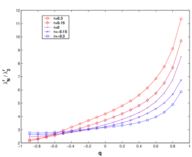
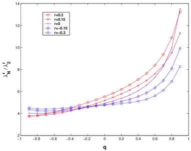
Figure 1: Eigenratio $\lambda_{N}/\lambda_{2}$ as function of q for scale free networks characterized by variable degree correlation: $r=[-0.3,-0.15,0,0.15,0.3]$. Left panel: $\gamma=2$, $N=1000$. Right panel: $\gamma=3$, $N=1000$.

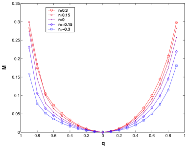
Figure 2: Maximum imaginary part of the spectrum of $\mathcal{L}$, M, as function of q for scale free networks characterized by variable degree correlation: $r=[-0.3,-0.15,0,0.15,0.3]$. Left panel: $\gamma=2$, $N=1000$. Right panel: $\gamma=3$, $N=1000$.

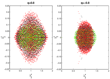
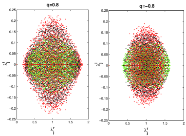
Figure 3: Spectrum of networks characterized by different degree correlation properties and degree of asymmetry. Each picture represents $\lambda_{j}^{i}$ vs $\lambda_{j}^{r}$, $j=1,2,...,N$. Green points are used for the spectrum of networks characterized by negative degree correlation ($r=-0.3$), black points are used for the spectrum of networks characterized by absence of correlation ($r=0$), red points for the spectrum of networks characterized by positive degree correlation ($r=+0.3$): (a) $\gamma=2$, $q=0.8$; (b) $\gamma=2$, $q=-0.8$; (c) $\gamma=3$, $q=0.8$; (d) $\gamma=3$, $q=-0.8$.

On the other hand, when $q\approx 0$, we observe a completely different picture with disassortative networks being characterized by better synchronizability properties (as already shown in [7]). The same behavior is also confirmed in the case of positive values of $q$, where the already better performance of disassortative networks is further enhanced through asymmetric coupling.

Thus the onset of two separate regimes emerges as varying $q$: the first one, in the case where there is a dominant interaction of the high-degree nodes on the low-degree ones, with assortative mixing representing a desirable property in terms of the network synchronizability; the second one, with symmetric coupling or directed from low-degree nodes to high-degree ones, where disassortative mixing represents the best choice in order to enhance the network synchronizability.

The behavior of the maximum imaginary part of the spectrum, $M$, as varying $q$, is show in Fig. 2. As expected, this is characterized by a minimum at $q=0$ (for which the coupling is symmetric) and increases as increasing the asymmetry over the network links. Note that for all values of $q\neq 0$, assortative (positively correlated) networks are characterized by higher values of $M$ when compared to their uncorrelated and disassortative counterparts.

A more exhaustive picture is provided in Fig. 3. Specifically here two configurations characterized by strong asymmetry ($q=0.8$ and $q=-0.8$) are compared for scale free networks with exponents $\gamma=\{2,3\}$, in terms of their spectra: $\lambda_{j}^{r}$ vs $\lambda_{j}^{i}$, for $j=1,2,..,N$. Networks characterized by different degree correlation properties are depicted with different colors: red for assortative mixing, green for disassortative, and black for no-correlation. Remind that the condition for increasing the network synchronizability is that the spectrum $\{\lambda_{j}\}$ for $j=2,..,N$ is contained in a region of the complex plane as small as possible.

This condition is clearly achieved for negative values of $q$ (compare respectively Figs. 3(a) with 3(b) and Figs. 3(c) with 3(d)). Note that in the case of $q=0.8$, the advantage of introducing negative degree correlation is undoubted, as both $R$ and $M$ are reduced and the green area is clearly smaller than the red one in Figs. 3(a) and 3(c). On the contrary, in the optimal regime where $q=-0.8$, the reduction of the range of the real values of the spectrum $\lambda_{j}^{r}$, $j=2,3,...,N$ is counterbalanced by an increase in the range of the imaginary parts $\lambda_{j}^{i}$, $j=2,3,...,N$, so that a more intricate phenomenology emerges.

Specifically, in such a case it becomes necessary to look at the specific form of the MSF under evaluation, in order to state the benefit of introducing degree correlation among the network connections. This should be taken into account, also with respect to variable forms of the MSF, when different choices of the functions $f$ and $h$ are taken into consideration.

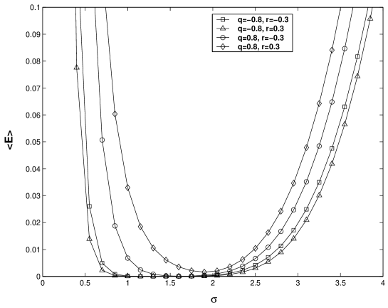
Figure 4: Synchronization error $\langle E\rangle$ as a function of the coupling strength $\sigma$ for a scale-free network of 1,000 Rössler oscillators (configuration model, $\gamma=2$). Evolution equations and parameters are specified in the text. Each point corresponds to an ensemble average over a set of 10 independent realizations. The asymmetry and correlation parameters are $q=0.8,r=0.3$ (diamonds), $q=0.8,r=-0.3$ (circles), $q=-0.8,r=0.3$ (triangles) and $q=-0.8,r=-0.3$ (squares). The numerical simulations support the qualitative scenario of the MSF: for positive (negative) values of $q$, synchronization is enhanced in disassortatively (assortatively) correlated graphs.

In order to confirm this qualitative description with an example, in the following we numerically simulate a network of 1,000 coupled chaotic Rössler oscillators. The dynamics of the system is ruled by Eq. 1, with $m=3$, ${x}=(x_{1},x_{2},x_{3})$, ${f}(x)=[-x_{2}-x_{3},\ x_{1}+0.165x_{2},\ 0.2+x_{3}(x_{1}-10)]$ and ${h}(x)=[x_{1},0,0]$.

The appearance of the synchronous state can here be monitored by looking at the vanishing of the time average (over a window $T$) of the synchronization error $\langle E\rangle=\frac{1}{T(N-1)}\sum_{j>1}\int_{t}^{t+T}||{x}_{j}-{x}_{1}||dt^{\prime}$. In the present case, we adopt as vector norm $||{x}||=|x_{1}|+|x_{2}|+|x_{3}|$.

Fig. 4 reports $\langle E\rangle$ vs. $\sigma$ for different networks topologies and degree correlations. It is easy to observe that the numerical simulations fully support the qualitative scenario of the MSF. Indeed, by comparing the synchronization effects in the cases $q=0.8,r=0.3$ (diamonds), $q=0.8,r=-0.3$ (circles), $q=-0.8,r=0.3$ (triangles) and $q=-0.8,r=-0.3$ (squares), one immediately realizes that for positive (negative) values of $q$, synchronization is enhanced in disassortatively (assortatively) correlated graphs.

In conclusion, in this paper we have regarded the network topology as the set of active connections present in the network, that is pairs $\{ij\}$, $i,j=1...N$, such that $\mathcal{A}_{ij}=1$. We analyzed the effects of varying the weights over the network connections (by making the parameter $q$ change) in order to investigate different levels of asymmetry. Moreover, we studied how variable degree correlation, while keeping the degree distribution unchanged, can favor or hinder the overall synchronization. While negative degree correlation was found to be a convenient network structural property in terms of synchronizability in the case of symmetric coupling ($q=0$) and of positive values of $q$ , a more intricate phenomenology was observed in the optimal situation, i.e. for low values of $q$. Specifically, in such a case an interesting balance between the width of the range of the real and imaginary parts of the eigenvalues has been observed.

We wish to emphasize that this issue could be of relevance in those applications where, because of different circumstances, synchronization may be or not be a desirable effect.

References

- [1] D.K. Arrowsmith, M. di Bernardo, and F. Sorrentino. Effects of variation of load distribution on network performance. Proc. IEEE ISCAS, Kobe, Japan, pages 3773–3776, 2005.
- [2] S. Boccaletti, V. Latora, Y. Moreno, M. Chavez, and D.U. Hwang. Complex networks: Structure and dynamics. Physics Reports, 424(4-5):175–308, 2006.
- [3] M. Boguña and R. Pastor-Satorras. Epidemic spreading in correlated complex networks. Phys. Rev. E, 66:047104, 2002.
- [4] M. Chavez, D.U. Hwang, A. Amann, H.G.E. Hentschel, and S. Boccaletti. Synchronization is enhanced in weighted complex networks. Phys. Rev. Lett., 94:218701, 2005.
- [5] Wu C.W. Synchronization in networks of nonlinear dynamical systems coupled via a directed graph. Nonlinearity, 18(3):1057–1064, 2005.
- [6] M. di Bernardo, F. Garofalo, and F. Sorrentino. Effects of degree correlation on the synchronizability of networks of nonlinear oscillators. International Journal of Bifurcation and Chaos (in press), 2006.
- [7] M. di Bernardo, F. Garofalo, and F. Sorrentino. Synchronizability and synchronization dynamics of weighed and unweighed scale free networks with degree mixing. International Journal of Bifurcation and Chaos (in press), 2006.
- [8] S.N. Dorogovtsev, A.V. Goltsev, and J.F.F. Mendes. Ising model on networks with an arbitrary distribution of connections. Phys.Rev. E, 66:016104, 2002.
- [9] S.N. Dorogovtsev, A.V. Goltsev, and J.F.F. Mendes. Potts model on complex networks. Eur. Phys. J. B, 38:177–182, 2004.
- [10] K.-I. Goh, B. Kahng, and D. Kim. Universal behavior of load distribution in scale-free networks. Phys. Rev. Lett., 87:278701, 2001.
- [11] R. Guimerà, A. Arenas, A. Díaz-Guilera, F. Vega-Redondo, and A. Cabrales. Optimal network topologies for local search with congestion. Phys.Rev.Lett., 89:248701, 2002.
- [12] D.U. Hwang, M. Chavez, A. Amann, and S. Boccaletti. Synchronization in complex networks with age ordering. Phys. Rev. Lett., 94:138701, 2005.
- [13] M. Molloy and B. Reed. A critical point for random graphs with a given degree sequence. Random Structures and Algorithms, (6):161–179, 1995.
- [14] C. Moore and M.E.J. Newman. Exact solution of site and bond percolation on small-world networks. Phys. Rev. E, 62(177):7059–7064, 2000.
- [15] A.E. Motter, C.S. Zhou, and J. Kurths. Enhancing complex-network synchronization. Europhys. Lett., 69:334, 2005.
- [16] A.E. Motter, C.S. Zhou, and J. Kurths. Network synchronization, diffusion, and the paradox of heterogeneity. Phys. Rev. E, 71:016116, 2005.
- [17] M.E.J. Newman. Scientific collaboration networks: II. shortest paths, weighted networks, and centrality. Phys. Rev. E, 64:016132, 2001.
- [18] M.E.J. Newman. Assortative mixing in networks. Phys. Rev. Lett., 89:208701, 2002.
- [19] M.E.J. Newman. The spread of epidemic disease on networks. Phys. Rev. E, 66:016128, 2002.
- [20] M.E.J. Newman. Mixing patterns in networks. Phys. Rev. E, 67:026126, 2003.
- [21] T. Nishikawa and A.E. Motter. Synchronization is optimal in non-diagonizable networks. Phys. Rev. E., 73:065106, 2006.
- [22] T. Nishikawa, A.E. Motter, Y. Lai, and F.C. Hoppensteadt. Heterogeneity in oscillator networks: Are smaller worlds easier to synchronize? Phys. Rev. Lett., 91:014101, 2003.
- [23] T. Ohira and R. Sawatari. Phase transition in a computer network traffic model. Phys. Rev. E, (58):193–195, 1998.
- [24] R. Pastor-Satorras and A. Vespignani. Epidemic spreading in scale-free networks. Phys. Rev. Lett., 86:3200, 2001.
- [25] L.M. Pecora and T.L. Carroll. Master stability functions for synchronized coupled systems. Phys. Rev. Lett., 80:2109–2112, 1998.
- [26] W. Lu and T. Chen. Synchronization analysis of linearly coupled networks of discrete time systems. Physica D, 198(1-2):148–168, 2004.