Kinetics of phase-separation in the critical spherical model and local scale-invariance

Abstract

The scaling forms of the space- and time-dependent two-time correlation and response functions are calculated for the kinetic spherical model with a conserved order-parameter and quenched to its critical point from a completely disordered initial state. The stochastic Langevin equation can be split into a noise part and into a deterministic part which has local scale-transformations with a dynamical exponent $z=4$ as a dynamical symmetry. An exact reduction formula allows to express any physical average in terms of averages calculable from the deterministic part alone. The exact spherical model results are shown to agree with these predictions of local scale-invariance. The results also include kinetic growth with mass conservation as described by the Mullins-Herring equation.

1 Introduction

A many-body system rapidly brought out of an initial equilibrium state by quenching it to either a critical point or into a coexistence region of the phase-diagramme where there are at least two equivalent equilibrium states undergoes ageing, that is the physical state depends on the time since the quench was performed and hence time-translation invariance is broken. Furthermore, either the competition between the distinct equilibrium states or else non-equilibrium critical dynamics leads to a slow dynamics, where observables depend non-exponentially on time. Both aspects of ageing can be conveniently studied through the two-time response and correlation functions defined as

$$R(t,s)=\left.\frac{\delta\langle\phi(t,\boldsymbol{r})\rangle}{\delta h(s,\boldsymbol{r})}\right|_{h=0}=s^{-a-1}f_{R}\left(\frac{t}{s}\right)\;\;,\;\;f_{R}(y)\stackrel{{\scriptstyle y\rightarrow\infty}}{{\sim}}y^{-{\lambda_{R}}/{z}}$$ (1.1)

$$C(t,s)=\bigl{\langle}\phi(t,\boldsymbol{r})\phi(s,\boldsymbol{r})\bigr{\rangle}=s^{-b}f_{C}\left(\frac{t}{s}\right)\;\;,\;\;f_{C}(y)\stackrel{{\scriptstyle y\rightarrow\infty}}{{\sim}}y^{-{\lambda_{C}}/{z}}$$ (1.2)

where $\phi(t,\boldsymbol{r})$ is the order-parameter at time $t$ and location $\boldsymbol{r}$ and $h$ is the conjugate magnetic field. These dynamical scaling forms (1.1,1.2) are expected to hold in the scaling limit where both $t,s\gg t_{\rm micro}$ and also $t-s\gg t_{\rm micro}$, where $t_{\rm micro}$ is some microscopic reference time. In writing those, it is implicitly assumed that the underlying dynamics is such that there is a single relevant length-scale $L=L(t)\sim t^{1/z}$, where $z$ is the dynamical critical exponent. Universality classes of ageing are defined through the values of the non-equilibrium exponents $a,b,\lambda_{C},\lambda_{R}$. for a non-vanishing initial value of the order-parameter, it is known that $\lambda_{C,R}$ may be related to the slip exponent introduced in [1] but there are no scaling relations with equilibrium exponents. For reviews, see e.g. [2, 3, 4, 5, 6].

A lot of attention has been devoted to the case where the underlying dynamics is such that there are no macroscopic conservation laws and in particular the order-parameter is non-conserved. In this situation, which is appropriate for the description of the ageing of magnets, results for the exponents $a,b,\lambda_{C},\lambda_{R}$ have been derived. Furthermore, it appears that simple dynamical scaling can be extended to a local scale-invariance, where the response functions transform covariantly under more general time-dependent rescalings of time and space [8]. In particular, this leads to explicit predictions for the scaling functions $f_{R}(y)$ (and also for $f_{C}(y)$ if $z=2$) which have been tested and confirmed in a large variety of systems, see [7] for a recent review.

In this paper, we are interested in carrying out a first case-study on the ageing and its local scale-invariance when the order-parameter is conserved. Physically, this may describe the phase-separation of binary alloys, where the order-parameter is given by the concentration difference of the two kinds of atoms. Another example are kinetic growth-processes at surfaces when mass conservation holds. One of the most simple models of this kind is the Mullins-Herring model [9, 10], which leads to a dynamical exponent $z=4$ and has recently been discussed in detail in [11].

Presently, there exist very few studies on ageing with a conserved order-parameter. In a numerical study of the $2D$ Ising model quenched to $T<T_{c}$, where $z=3$, Godrèche, Krzakala and Ricci-Tersenghi [12] calculated the scaling function $f_{C}(y)$ which remarkably shows a cross-over between a first power-law decay $f_{C}(y)\sim y^{-\lambda_{C}^{\prime}/z}$ for intermediate values of $y$ to the final asymptotic behaviour (1.2) for $y\gg 1$. They find a value of $\lambda_{C}^{\prime}=2.5$, whereas the value for $\lambda_{C}$ is much smaller with $\lambda_{C}=1$. On the other hand, Sire [13] calculated $f_{C}(y)$ exactly in the critical spherical model ($T=T_{c}$), where $z=4$, and found a single power-law regime. For a review, see [4].

Here, we shall revisit the spherical model with a conserved order-parameter, quenched to $T=T_{c}$. Besides reviewing the calculation of the two-time correlation function we shall also provide the exact solution for the two-time response function. This will be described in section 2. Our main focus will be to show how these exact results can be understood from an extension of dynamical scaling to local scale-invariance (LSI) with $z=4$. In section 3, we recall the main results of LSI for that case and in particular write down a linear partial differential equation of which this LSI is a dynamical symmetry. In section 4, we consider the Langevin equation which describes the kinetics with a conserved order-parameter (model B in the Halperin-Hohenberg classification) and show for the case at hand how the Langevin-equation can be split into a ‘deterministic’ and a ‘noise’ part, so that all averages to be calculated can be exactly reduced to quantities to be found in a noise-less theory. Local scale-invariance directly determines the latter, as we shall see in section 5, where we can finally compare with the exact spherical model results of section 2. This is, together with the earlier study of the Mullins-Herring model in [11], the first example where local scale-invariance can be confirmed for an exactly solvable model with dynamical exponent $z\neq 2$. Our conclusions are formulated in section 6. Some technical points are reported in the appendices. In appendix A we derive the two-point function from the symmetry operators and in appendix B we calculate solution of an integral which appears frequently in our computations. In an outlook beyond the present specific context, we discuss in appendix C the autoresponse function for values of $z$ different from $4$. In appendix D we discuss the most simple possible model, namely a free particle submitted to conserved noise. This serves as a further illustration of some of the space-time properties of the conserved spherical model.

2 The spherical model with a conserved order-parameter

The spherical model was conceived in 1953 by Berlin and Kac as a mathematical model for strongly interacting spins which is yet easily solvable and it has indeed served a useful rôle in providing exact results in a large variety of interesting physical situations. It may be defined in terms of a real spin variable $S(t,\boldsymbol{x})$ attached to each site $\boldsymbol{x}$ of a hypercubic lattice $\Lambda\subset\mathbb{Z}^{d}$ and depending on time $t$, subject to the (mean) spherical constraint

$$\left\langle\sum_{\boldsymbol{x}\in\Lambda}S(t,\boldsymbol{x})^{2}\right\rangle={\cal N}$$ (2.1)

where $\cal N$ is the number of sites of the lattice. The Hamiltonian is ${\cal H}=-\sum_{(\boldsymbol{x},\boldsymbol{y})}S_{\boldsymbol{x}}S_{\boldsymbol{y}}$ where the sum is over pairs of nearest neighbours. The kinetics is assumed to be given by a Langevin equation of model B type

$$\partial_{t}S(t,\boldsymbol{x})=-\nabla_{\boldsymbol{x}}^{2}\left[\nabla_{\boldsymbol{x}}^{2}S(t,\boldsymbol{x})+\mathfrak{z}(t)S(t,\boldsymbol{x})+h(t,\boldsymbol{x})\right]+\eta(t,\boldsymbol{x})$$ (2.2)

where $\mathfrak{z}(t)$ is the Lagrange multiplier fixed by the mean spherical constraint and the coupling to the heat bath with the critical temperature $T_{c}$ is described by a Gaussian noise $\eta$ of vanishing average and variance

$$\left\langle\eta(t,\boldsymbol{x})\eta(t^{\prime},\boldsymbol{x}^{\prime})\right\rangle=-2T_{c}\nabla_{\boldsymbol{x}}^{2}\delta(t-t^{\prime})\delta(\boldsymbol{x}-\boldsymbol{x}^{\prime}).$$ (2.3)

and $h(t,\boldsymbol{x})$ is a small external magnetic field. Here the derivative on the right-hand side of (2.3) expresses the fact that the noise is chosen in such a way that it does not break the conservation law. On the other hand, there are physical situations such as surface growth with mass conservation, where this is not the case. The non-conserved Mullins-Herring model [9, 10] is given by equation (2.2) with $\mathfrak{z}=0$ and the noise correlator $\langle\eta(t,\boldsymbol{x})\eta(t^{\prime},\boldsymbol{x}^{\prime})\rangle=2T_{c}\,\delta(t-t^{\prime})\delta(\boldsymbol{x}-\boldsymbol{x}^{\prime})$, see [11] for details. Here we shall study the conserved Mullins-Herring model, that is equation (2.2) with $\mathfrak{z}(t)=0$ and the noise correlator (2.3). A similar remark applies on the way we included the perturbation $h(t,\boldsymbol{x})$. Here we study the case, where the perturbation does not break the conservation law.

The spherical constraint is taken into account through the Lagrange multiplier $\mathfrak{z}(t)$ which has to be computed self-consistently. These equations have already been considered several times in the literature [18, 19, 13].

2.1 The correlation function

We repeat here the main steps of the calculation of the correlation function [18, 19, 13]. Equation (2.2) with $h(t,\boldsymbol{x})=0$ is readily solved in Fourier-space, yielding

$$\widehat{S}(t,\boldsymbol{k})=\left[\widehat{S}(0,\boldsymbol{k})+\int_{0}^{t}\!{\rm d}\tau\>\exp\Big{(}\omega(\tau,\boldsymbol{k})\Big{)}\eta(\tau,\boldsymbol{k})\right]\exp\Big{(}-\omega(t,\boldsymbol{k})\Big{)}$$ (2.4)

where $\widehat{S}(t,\boldsymbol{k})$ denotes the spatial Fourier transformation of $S(t,\boldsymbol{r})$ and

$$\omega(t,\boldsymbol{k})=k^{4}t-k^{2}\int_{0}^{t}\!{\rm d}\tau\,\mathfrak{z}(\tau),\qquad\mbox{with}\qquad k:=|\boldsymbol{k}|$$ (2.5)

Next, $\omega(t,\boldsymbol{k})$ is determined from the spherical constraint. This is easiest in the continuum limit where spatial translation-invariance leads to $\langle S^{2}(t,\boldsymbol{x})\rangle=(2\pi)^{-d}\int^{\Lambda}\!{\rm d}\boldsymbol{k}\,\langle\widehat{S}(t,-\boldsymbol{k})\widehat{S}(t,\boldsymbol{k})\rangle=1$ where $\Lambda$ is the inverse of a lattice cutoff. This has already been analysed in the literature [18, 19, 13], with the result

$$\omega(t,\boldsymbol{k})=k^{4}t-\mathfrak{g}_{d}k^{2}t^{{1}/{2}}$$ (2.6)

where the constant $\mathfrak{g}_{d}$ is determined by the condition [18]

$$\int_{0}^{\infty}\!{\rm d}x\,x^{d-1}\left\{2x^{2}\int_{0}^{1}\!{\rm d}y\,\exp\left[-2x^{4}(1-y)+2\mathfrak{g}_{d}x^{4}(1-\sqrt{y\,})\right]-\frac{1}{x^{2}}\right\}=0$$ (2.7)

In particular, $\mathfrak{g}_{d}=0$ for $d>4$ and asymptotic forms for $d\to 2$ and $d\to 4$ are listed in [18]. Then from (2.4) the two-time correlator $\widehat{C}(t,s,\boldsymbol{k}):=\Big{\langle}\widehat{S}(t,-\boldsymbol{k})\widehat{S}(s,\boldsymbol{k})\Big{\rangle}$ is straightforwardly derived

$$\widehat{C}(t,s,\boldsymbol{k})=s_{0}(\boldsymbol{k})^{2}\exp\Big{(}-\omega(t,\boldsymbol{k})-\omega(s,\boldsymbol{k})\Big{)}$$ (2.8)

$$+ 2T_{c}\int_{0}^{s}\!{\rm d}u\>k^{2}\exp\Big{(}-\omega(t,\boldsymbol{k})-\omega(s,\boldsymbol{k})+2\omega(u,\boldsymbol{k})\Big{)}$$

where $s_{0}(\boldsymbol{k})^{2}:=\Big{\langle}\widehat{S}(0,-\boldsymbol{k})\widehat{S}(0,\boldsymbol{k})\Big{\rangle}$. Transforming back to direct space, one obtains

$$C(t,s;\boldsymbol{r})=A_{1}(t,s;\boldsymbol{r})+A_{2}(t,s;\boldsymbol{r})$$ (2.9)

where $A_{1}(t,s;\boldsymbol{r})$ and $A_{2}(t,s;\boldsymbol{r})$ are the inverse Fourier transforms of the first and the second line of the right-hand side of equation (2.8), respectively. They are explicitly given by the following expressions, where we use the shorthand $y:=t/s$

$$A_{1}(t,s;\boldsymbol{r}) = (t+s)^{-{d}/{4}}\int_{\mathbb{R}^{d}}\frac{{\rm d}\boldsymbol{k}}{(2\pi)^{d}}\,s_{0}(\boldsymbol{k})^{2}\exp\left(-\frac{{\rm i}\boldsymbol{k}\cdot\boldsymbol{r}}{(t+s)^{{1}/{4}}}\right)$$

$$\times\exp\left(-k^{4}+\mathfrak{g}_{d}k^{2}\frac{y^{{1}/{2}}+1}{(y+1)^{{1}/{2}}}\right)$$

and

$$A_{2}(t,s;\boldsymbol{r}) = 2T_{c}s^{-(d-2)/4}\int_{0}^{1}\!{\rm d}\theta\;(y+1-2\theta)^{-(d+2)/4}\int_{\mathbb{R}^{d}}\frac{{\rm d}\boldsymbol{k}}{(2\pi)^{d}}\,k^{2}$$

$$\times\exp\left(-\frac{{\rm i}\boldsymbol{k}\cdot\boldsymbol{r}}{(s(y+1-2\theta))^{{1}/{4}}}\right)\exp\left(-k^{4}+\mathfrak{g}_{d}k^{2}\left(\frac{y^{1/2}+1-2\theta^{1/2}}{(y+1-2\theta)^{{1}/{2}}}\right)\right)$$

The term $A_{2}(t,s;\boldsymbol{r})$ is the dominating one in the scaling regime where $t,s\to\infty$ and $y=t/s$ is kept fixed. There we recover the scaling form (1.2) with $b=(d-2)/4$. The explicit expression for the scaling function $f_{C}(y)$ is quite cumbersome but, if the last term in the second exponential in eq. (2.1) can be treated as a constant, one has, up to normalisation

$$f_{C}(y)\sim\left\{\begin{array}[]{cc}\frac{8T_{c}}{2-d}\left[(y-1)^{(2-d)/4}-(y+1)^{(2-d)/4}\right]&\qquad\mbox{\rm;~{}~{} $d>2$}\\ 2T_{c}\ln\left(\frac{y-1}{y+1}\right)&\qquad\mbox{\rm;~{}~{} $d=2$}\end{array}\right.$$ (2.12)

This is exact for the spherical model for $d>4$, since then $\mathfrak{g}_{d}=0$. Equation (2.12) also applies to the Mullins-Herring equation for any $d\geq 1$ (since here $\mathfrak{z}=0$, in this case $\mathfrak{g}_{d}=0$ exactly). For $y$ sufficiently large, the above condition is also approximately satisfied. In any case, in the limit $y\to\infty$ we can read off the autocorrelation exponent $\lambda_{C}=d+2$.

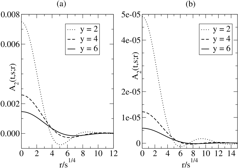
Figure 1: Scaling of the spatio-temporal correlation function $C(t,s;\boldsymbol{r})\simeq A_{2}(t,s;\boldsymbol{r})$ with $s=20$ and for several values of $y=t/s$ for (a) $d=3$ (left panel) and (b) $d=5$ (right panel).

The scaling behaviour of the spatio-temporal two-time correlator is illustrated in figure 1. We see that for relatively small values of $y=t/s$, the correlation function does not decay monotonously towards zero, but rather displays oscillations whose amplitude decays with $|\boldsymbol{r}|s^{-1/4}$. This behaviour is quite close to the well-known one for the equal-time correlation function. As $y$ increases, these oscillations become less pronounced. There is no apparent qualitative difference between the cases $d<4$ and $d>4$.

2.2 The response function

The response function can be computed in a way similar to the non-conserved case [20]. Equation (2.2) is solved in Fourier space yielding an equation similar to (2.4)

$$\widehat{S}(t,\boldsymbol{k}) = \Big{[}\widehat{S}(0,\boldsymbol{k})+\int_{0}^{t}\!{\rm d}\tau\,\exp\Big{(}\omega(\tau,\boldsymbol{k})\Big{)}$$ (2.13)

$$\times\Big{(}\widehat{\eta}(\tau,\boldsymbol{k})+k^{2}\widehat{h}(\tau,\boldsymbol{k})\Big{)}\Big{]}\exp(-\omega(t,\boldsymbol{k}))$$

From this the Fourier transform of the response function is computed as $\widehat{R}(t,s,\boldsymbol{k})={\delta\langle\widehat{S}(t,\boldsymbol{k})\rangle}/{\delta h(s,-\boldsymbol{k})}$. Transforming the result back to direct space, we obtain for $t>s$

$$R(t,s;\boldsymbol{r}) = (t-s)^{-(d+2)/4}\int_{\mathbb{R}^{d}}\frac{{\rm d}\boldsymbol{k}}{(2\pi)^{d}}k^{2}\exp\left(-\frac{{\rm i}\boldsymbol{k}\cdot\boldsymbol{r}}{(t-s)^{{1}/{4}}}\right)$$ (2.14)

$$\times\exp\left(-k^{4}+\mathfrak{g}_{d}k^{2}\frac{y^{{1}/{2}}-1}{(y-1)^{{1}/{2}}}\right)$$

It is easy to see that the scaling form (1.2) holds with $a=(d-2)/4=b$. For large values of $y$ the scaling function $f_{R}(y)$ is given by

$$f_{R}(y)\sim(y-1)^{-{(d+2)}/{4}}.$$ (2.15)

Again, for $d>4$ this expression is exact up to a prefactor. The value of the autoresponse exponent therefore is, for $d>2$

$$\lambda_{R}=d+2=\lambda_{C}$$ (2.16)

in agreement with field-theoretical expectations for the O($n$) model [4].

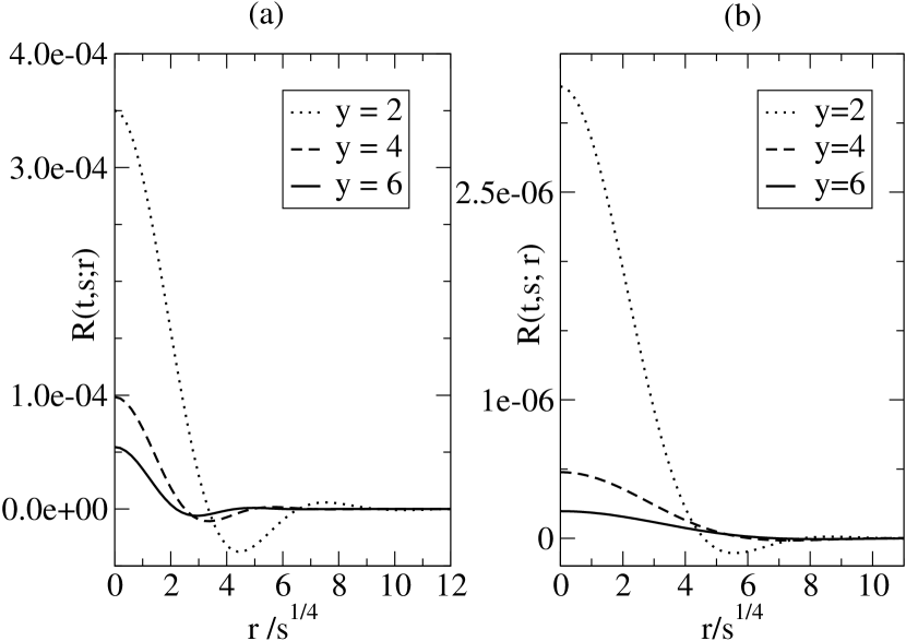
Figure 2: Scaling of the spatio-temporal response function $R(t,s;\boldsymbol{r})$ for $s=20$ and several values of $y=t/s$ for $d=3$ (left panel) and $d=5$ (right panel).

It is instructive to consider the full space-time response function explicitly for the case that $\mathfrak{g}_{d}=0$, that is for $d>4$ in the spherical model and for any $d$ in the Mullins-Herring equation. The integral in (2.14) is done in appendix B and we find

$$R(t,s;\boldsymbol{r})=\frac{\sqrt{\pi}}{2^{3d/2}\pi^{d/2}\Gamma(d/4)}\>(t-s)^{-{(d+2)}/{4}}\left[{{}_{0}F_{2}}\left(\frac{1}{2},\frac{d}{4};\frac{r^{4}}{256\,(t-s)}\right)\right.$$ (2.17)

$$- \left.\frac{8}{d}\frac{\Gamma\left(\frac{d}{4}+1\right)}{\Gamma\left(\frac{d}{4}+\frac{1}{2}\right)}\left(\frac{r^{2}}{16\sqrt{t-s}}\right){{}_{0}F_{2}}\left(\frac{3}{2},\frac{d}{4}+\frac{1}{2};\frac{r^{4}}{256\,(t-s)}\right)\right]$$

This expression will be useful later for direct comparison with the results obtained from the theory of local scale-invariance. For $\mathfrak{g}_{d}\neq 0$ it is more convenient to use the integral representation (2.14). In figure 2 we display the spatio-temporal response function. In contrast to the non-conserved case for a fixed value of $y=t/s$ there are decaying oscillations with the scaling variable $|\boldsymbol{r}|s^{-1/4}$. These oscillations disappear rapidly when $y$ is increased. This qualitative behaviour also arises, as we show in appendix D, for the simple random walk with a conserved noise.

Having found both correlation and response functions, we can also calculate the fluctuation-dissipation ratio $X(t,s)=TR(t,s)(\partial C(t,s)/\partial s)^{-1}$ which measures the distance from equilibrium [21]. In particular, we find for the fluctuation-dissipation limit

$$X_{\infty}=\lim_{s\to\infty}\left(\lim_{t\to\infty}X(t,s)\right)=\frac{1}{2}$$ (2.18)

in agreement with the known result [4] of the conserved $n\to\infty$ limit of the O($n$) model.

3 Symmetries of the deterministic equation

Before we can examine dynamical symmetries in Langevin equations, we need some background material on the dynamical symmetries of the deterministic part of such equations. Therefore, we recall in this section first some facts about Schrödinger-invariance which describes an extension of dynamical scaling for a dynamical exponent $z=2$. As shown earlier [8], an analogous extension can be built for $z\neq 2$ and we shall write down the relevant generators for this local scale-invariance for $z=4$.

The physical starting point is the covariance of $n$-point functions such as the correlator $F^{(n)}(t_{1},\ldots,t_{n};\boldsymbol{r}_{1},\ldots,\boldsymbol{r}_{n},)=\langle\phi_{1}(t_{1},\boldsymbol{r}_{1})\ldots,\phi_{n}(t_{n},\boldsymbol{r}_{n})\rangle$ under the rescaling of spatial and temporal coordinates

$$F^{(n)}(b^{z}t_{1},\ldots,b^{z}t_{n};b\boldsymbol{r}_{1},\ldots,b\boldsymbol{r}_{n})=b^{-(x_{1}+\ldots+x_{n})}F^{(n)}(t_{1},\ldots t_{n};\boldsymbol{r}_{1},\ldots,\boldsymbol{r}_{n})$$ (3.1)

where the $x_{i}$ are the scaling dimensions of the fields $\phi_{i}$ and $z$ is the dynamical exponent. By analogy with conformal invariance at equilibrium, one asks whether an extension of dynamical scaling to local scale-transformations with a space-time dependent rescaling factor $b(t,\boldsymbol{r})$ might be possible. The most simple case is the one of Schrödinger-invariance which describes the dynamical symmetries of the linear diffusion equation (or free Schrödinger equation)

$$\hat{S}_{\rm sch}\phi(\boldsymbol{r},t)=0,\qquad\mbox{with}\quad\hat{S}_{\rm sch}:=\lambda\partial_{t}-\frac{1}{4}\nabla_{\boldsymbol{r}}^{2}$$ (3.2)

where the parameter $\lambda$ is related to the inverse diffusion constant. The symmetry group of this equation, that is the largest group of transformations carrying solutions of (3.2) to other solutions, was already found 1882 by Lie and is the well-known Schrödinger group Sch($d$), see [22]. It transforms coordinates as $(t,\boldsymbol{r})\mapsto(t^{\prime},\boldsymbol{r}^{\prime})=g(t,\boldsymbol{r})$ with

$$\boldsymbol{r}^{\prime}=\frac{\mathcal{R}\boldsymbol{r}+\boldsymbol{v}t+\boldsymbol{a}}{\tilde{\gamma}t+\tilde{\delta}}\;\;,\;\;t^{\prime}=\frac{\tilde{\alpha}t+\tilde{\beta}}{\tilde{\gamma}t+\tilde{\delta}}\;\;;\;\;\tilde{\alpha}\tilde{\delta}-\tilde{\beta}\tilde{\gamma}=1$$ (3.3)

where $\mathcal{R}$ is a rotation matrix and $\boldsymbol{v},\boldsymbol{a},\tilde{\alpha},\tilde{\beta},\tilde{\gamma}$ and $\tilde{\delta}$ are parameters. Evidently, the dynamical exponent is $z=2$. The solutions of (3.2) transform as

$$\phi(t,\boldsymbol{r})\rightarrow(T_{g}\phi)(t,\boldsymbol{r})=f_{g}[g^{-1}(t,\boldsymbol{r})]\phi(g^{-1}(t,\boldsymbol{r}))$$ (3.4)

where the companion function $f_{g}$ is known explicitly [22]. A field transforming as (3.4) is called quasiprimary. The generators of the Schrödinger group form a Lie algebra $\mathfrak{sch}_{d}=\mbox{\rm Lie({\sl Sch}($d$))}$ and it can be shown that a $n$-point correlator built from quasiprimary fields must satisfy the conditions

$$\sum_{i=1}^{n}\mathcal{X}_{i}\;\left\langle\phi_{1}(t_{1},\boldsymbol{r}_{1})\ldots\phi_{n}(t_{n},\boldsymbol{r}_{n})\right\rangle=0$$ (3.5)

where $\mathcal{X}_{i}$ stands for any generator of $\mathfrak{sch}_{d}$ which acts on the field $\phi_{i}$. For example, eq. (3.5) fixes the two-point function of quasiprimary fields completely [23].

Following [8], we now write the generalisation of this to the case when $z=4$ which has already been started in [11]. Consider the ‘Schrödinger operator’

$$\hat{S}:=-\lambda\partial_{t}+\frac{1}{16}\left(\nabla_{\boldsymbol{r}}^{2}\right)^{2}.$$ (3.6)

which we shall encounter in the context of the conserved spherical model and where obviously $z=4$. Using the shorthands $\boldsymbol{r}\cdot\partial_{\boldsymbol{r}}:=\sum_{k=1}^{d}r_{k}\,\partial_{r_{k}}$,$\nabla_{\boldsymbol{r}}^{2}:=\sum_{k=1}^{d}\partial_{r_{k}}^{2}$ and $\boldsymbol{r}^{2}:=\sum_{k=1}^{d}r_{k}^{2}$, the infinitesimal generators of local scale-transformations read (using a notation analogous to [8])

$$X_{-1} := -\partial_{t}$$

$$X_{0} := -t\partial_{t}-\frac{1}{4}\,\boldsymbol{r}\cdot\partial_{\boldsymbol{r}}-\frac{x}{4}$$

$$X_{1} := -t^{2}\partial_{t}-\frac{x}{2}t-\lambda\boldsymbol{r}^{2}\,(\nabla_{\boldsymbol{r}}^{2})^{-1}-\frac{1}{2}\,t\boldsymbol{r}\cdot\partial_{\boldsymbol{r}}$$ (3.7)

$$+4\gamma\,\left(\boldsymbol{r}\cdot\partial_{\boldsymbol{r}}\right)\,\left(\nabla_{\boldsymbol{r}}^{2}\right)^{-2}+2\gamma(d-4)\left(\nabla_{\boldsymbol{r}}^{2}\right)^{-2}$$

$$R^{(i,j)} := r_{i}\partial_{r_{j}}-r_{j}\partial_{r_{i}}\;\;;\;\;\mbox{\rm where $1\leq i<j\leq d$}$$

$$Y^{(i)}_{-1/4} = -\partial_{r_{i}}$$

$$Y^{(i)}_{3/4} = -t\partial_{r_{i}}-4\lambda r_{i}\left(\nabla_{\boldsymbol{r}}^{2}\right)^{-1}+8\gamma\,\partial_{r_{i}}\left(\nabla_{\boldsymbol{r}}^{2}\right)^{-2}$$

where $x$ is the scaling dimension of the fields on which these generators act and $\gamma,\lambda$ are further field-dependent parameters. Here, the generators $X_{\pm 1,0}$ correspond to projective changes in the time $t$, the generators $Y^{(i)}_{n-1/4}$ are space-translations, generalised Galilei-transformations and so on and $R^{(i,j)}$ are spatial rotations. In writing these generators, the following properties of the derivative $\partial_{r}^{\alpha}$ are assumed

$$\partial_{r}^{\alpha}\partial_{r}^{\beta}=\partial_{r}^{\alpha+\beta}\;\;,\;\;{}\left[\partial_{r}^{\alpha},r\right]=\alpha\partial_{r}^{\alpha-1}$$ (3.8)

and which can be justified in terms of fractional derivatives as shown in detail in appendix A of [8]. The operator $(\nabla_{\boldsymbol{r}}^{2})^{-1}$ can then be defined formally as follows. For example, in $d=2$ dimensions, we have

$$(\nabla_{\boldsymbol{r}}^{2})^{-1}:=(\partial_{r_{x}}^{2}+\partial_{r_{y}}^{2})^{-1}:=\sum_{n=0}^{\infty}(-1)^{n}\partial_{r_{x}}^{-2-2n}\partial_{r_{y}}^{2n}$$ (3.9)

The remaining negative powers of $\nabla_{\boldsymbol{r}}$ are then defined by concatenation, e.g. $(\nabla_{\boldsymbol{r}}^{2})^{-2}=(\nabla_{\boldsymbol{r}}^{2})^{-1}\cdot(\nabla_{\boldsymbol{r}}^{2})^{-1}$. We easily verify the following commutation relations for $n\in\mathbb{Z}$

$${[}(\nabla_{\boldsymbol{r}}^{2})^{n},r_{i}] = n\,\partial_{r_{i}}(\nabla_{\boldsymbol{r}}^{2})^{n-1}$$ (3.10)

$${[}(\nabla_{\boldsymbol{r}}^{2})^{n},\boldsymbol{r}^{2}] = 2n\,(\boldsymbol{r}\cdot\partial_{\boldsymbol{r}})\,(\nabla_{\boldsymbol{r}}^{2})^{n-1}+n\,(n-2+d)(\nabla_{\boldsymbol{r}}^{2})^{n-1}$$ (3.11)

The generators eq. (3.7) describe dynamical symmetries of the ‘Schrödinger operator’ (3.6). This can be seen from the commutators of $\hat{S}$ and the generators ${\cal X}$ from eq. (3.7). Straightforward, but a little tedious calculations give, analogously to [8]

$${}[\hat{S},X_{-1}] = 0\;\;,\;\;[\hat{S},Y^{(i)}_{-1/4}]\>=\>0\;\;,\;\;[\hat{S},Y^{(i)}_{3/4}]\>=\>0$$

$${}[\hat{S},X_{0}] = -\hat{S}\;\;,\;\;[\hat{S},R^{(i,j)}]\>=\>0$$ (3.12)

This means that for a solution of the ‘Schrödinger equation’ $\hat{S}\phi=0$ the transformed function ${\cal X}\phi$ is again solution of the ‘Schrödinger equation’. For the commutator with $X_{1}$ we find

$${}[\hat{S},X_{1}]=-2t\hat{S}+\frac{\lambda}{2}\left(x-\frac{d}{2}-1+\frac{2\gamma}{\lambda}\right)$$ (3.13)

hence a dynamical symmetry is found if the field $\phi$ has the scaling dimension

$$x=\frac{d}{2}+1-\frac{2\gamma}{\lambda}$$ (3.14)

which for $d=1$ reproduces the result of [8]. Generalising from conformal or Schrödinger-invariance, quasiprimary fields transform covariantly and their $n$-point functions will again satisfy eq. (3.5). A quasiprimary field is now characterised by its scaling dimension $x_{i}$ and the further parameters $\gamma_{i},\lambda_{i}$. For example, any two-point function $F^{(2)}=\langle\phi_{1}\phi_{2}\rangle$ built from two quasiprimary fields $\phi_{1,2}$ is completely fixed by solving the conditions (3.5) for the generators in (3.7). We quote the result and refer to appendix A for the details of the calculation.

$$F^{(2)}(t-s,\boldsymbol{x}-\boldsymbol{y}):=\langle\phi_{1}(t,\boldsymbol{x})\phi_{2}(s,\boldsymbol{y})\rangle$$ (3.15)

$$= \delta_{x_{1},x_{2}}\delta_{\lambda_{1},-\lambda_{2}}\delta_{\gamma_{1},-\gamma_{2}}\,(t-s)^{-{x}/{2}}\sum_{s\in\mathcal{E}^{\prime}}c_{s}\phi^{(s)}\left(|\boldsymbol{x}-\boldsymbol{y}|(t-s)^{-1/4}\right)$$

Here $\phi^{(s)}(u)$ are scaling functions, the $c_{s}$ are free parameters and the set $\mathcal{E}^{\prime}$ is defined as follows

$$\mathcal{E}^{\prime}:=\left\{\begin{array}[]{lcl}\{2,4\}&\mbox{if}&d>4\\ \{2,4,4-d\}&\mbox{if}&2<d\leq 4\\ \{2,4,2-d,4-d\}&\mbox{if}&d\leq 2\end{array}\right.$$ (3.16)

We shall see later that boundary conditions may impose further conditions on the $c_{s}$. The functions $\phi^{(s)}(u)$ are given by the series, convergent for all $|u|<\infty$

$$\phi^{(s)}(u)=\sum_{\ell=0}^{\infty}b_{\ell}^{(s)}u^{4\ell+s-4}.$$ (3.17)

with the coefficients $b_{\ell}^{(s)}$

$$b_{\ell}^{(s)}=2^{4}\frac{\Gamma(\frac{s}{2}+1)\Gamma(\frac{s}{2}+\frac{d}{2})}{\Gamma(\frac{s+d}{4}-\frac{1}{2}-\frac{\gamma}{\lambda})}\cdot\frac{\Gamma(\ell+\frac{s+d}{4}-\frac{1}{2}-\frac{\gamma}{\lambda})}{\Gamma(2\ell+\frac{s}{2}-1)\Gamma(2\ell+\frac{s}{2}+\frac{d}{2}-2)}\left(-\lambda\right)^{\ell}$$ (3.18)

4 Local scale-invariance

4.1 General remarks

Consider the following stochastic Langevin equation

$$\partial_{t}\phi=-\frac{1}{16\lambda}\nabla_{\boldsymbol{r}}^{2}\Big{(}-\nabla_{\boldsymbol{r}}^{2}\phi+v(t)\phi\Big{)}+\eta$$ (4.1)

where the noise correlator respects the global conservation law

$$\langle\eta(\boldsymbol{r},t)\eta(\boldsymbol{r}^{\prime},t^{\prime})\rangle=-\frac{T}{8\lambda}\nabla_{\boldsymbol{r}}^{2}\delta(\boldsymbol{r}-\boldsymbol{r}^{\prime})\delta(t-t^{\prime})$$ (4.2)

Here and in what follows, we shall often suppress the arguments of the fields for the sake of simplicity, if no ambiguity arises. We shall adopt the standard field-theoretical setup for the description of Langevin equations, see e.g. [24, 25, 26] for introductions. The Janssen- de Domincis action can be written in terms of the order-parameter field $\phi$ and its conjugate response field $\widetilde{\phi}$ and reads

$$\mathcal{J}[\phi,\widetilde{\phi}] = \int\!{\rm d}u{\rm d}\boldsymbol{R}\,\left[\widetilde{\phi}\left(\partial_{u}-\frac{1}{16\lambda}\nabla_{\boldsymbol{R}}^{2}\Big{(}\nabla_{\boldsymbol{R}}^{2}-v(u)\Big{)}\right)\phi\right]$$

$$+ \frac{T}{16\lambda}\int\!{\rm d}u{\rm d}\boldsymbol{R}\>\widetilde{\phi}(u,\boldsymbol{R})\,(\nabla_{\boldsymbol{R}}^{2}\widetilde{\phi})(u,\boldsymbol{R})$$

to which an extra term describing the initial noise must be added, by analogy with the non-conserved case [27, 28]

$$\mathcal{J}_{init}[\phi,\widetilde{\phi}]=\frac{1}{2}\int\!{\rm d}\boldsymbol{R}{\rm d}\boldsymbol{R}^{\prime}\,\widetilde{\phi}(0,\boldsymbol{R})\Big{\langle}\phi(0,\boldsymbol{R})\phi(0,\boldsymbol{R}^{\prime})\Big{\rangle}\widetilde{\phi}(0,\boldsymbol{R}^{\prime})$$ (4.4)

Averages of an observable $\mathcal{O}$ are defined as usual by functional integrals with weight $\exp(-\mathcal{J}[\phi,\widetilde{\phi}])$, viz.

$$\langle\mathcal{O}\rangle:=\int\mathcal{D}[\phi]\mathcal{D}[\widetilde{\phi}]\mathcal{O}\exp(-\mathcal{J}[\phi,\widetilde{\phi}])$$ (4.5)

We decompose the action, in the same way as done in [28] for the non-conserved case, into a deterministic and a noise part, that is

$$\mathcal{J}[\phi,\widetilde{\phi}]=\mathcal{J}_{0}[\phi,\widetilde{\phi}]+\mathcal{J}_{\rm b}[\widetilde{\phi}]$$ (4.6)

with

$$\mathcal{J}_{0}[\phi,\widetilde{\phi}]=\int\!{\rm d}u{\rm d}\boldsymbol{R}\,\left[\widetilde{\phi}\left(\partial_{u}-\frac{1}{16\lambda}\nabla_{\boldsymbol{R}}^{2}\Big{(}\nabla_{\boldsymbol{R}}^{2}-v(u)\Big{)}\right)\phi\right]$$ (4.7)

and ${\cal J}_{\rm b}={\cal J}_{\rm th}+{\cal J}_{\rm init}$ where

$$\mathcal{J}_{\rm th}[\widetilde{\phi}]=\frac{T}{16\lambda}\int\!{\rm d}u{\rm d}\mathbf{R}\>\widetilde{\phi}(u,\mathbf{R})\Big{(}\nabla_{\boldsymbol{R}}^{2}\widetilde{\phi}\Big{)}(u,\mathbf{R})$$ (4.8)

The point of this split-up is, as we shall show, that the action ${\cal J}_{0}[\phi,\widetilde{\phi}]$ has nontrivial symmetry properties, in contrast to the full action ${\cal J}[\phi,\widetilde{\phi}]$, where these symmetries are destroyed by the noise. We call the theory with respect to ${\cal J}_{0}[\phi,\widetilde{\phi}]$ noise-free and denote averages taken with respect to ${\cal J}_{0}[\phi,\widetilde{\phi}]$ only by $\langle\ldots\rangle_{0}$. Averages of the full theory can then be computed by formally expanding around the noise-free theory

$$\Big{\langle}\mathcal{O}\Big{\rangle}=\left\langle\mathcal{O}\exp(-\mathcal{J}_{\rm b}[\widetilde{\phi}])\right\rangle_{0}$$ (4.9)

The noise-free theory has a Gaussian structure, if we consider the two-component field $\Psi=\left({\phi\atop\widetilde{\phi}}\right)$. Then the factor $\exp(-{\cal J}_{0}[\phi,\widetilde{\phi}])$ can be written as $\exp(-\int\!{\rm d}u{\rm d}\boldsymbol{R}{\rm d}u^{\prime}{\rm d}\boldsymbol{R}^{\prime}\,\Psi^{t}\mathsf{A}\Psi)$ with an antidiagonal matrix $\mathsf{A}$. From this, two important facts can be deduced:

1. Wick’s Theorem holds [30]. That is, we can write the $2n$-point function as

   $$\Big{\langle}\phi(t_{1},\boldsymbol{r}_{1})\ldots\phi_{2n}(t_{2n},\boldsymbol{r}_{2n})\Big{\rangle}_{0}=\sum_{\mbox{all possible pairings}\atop\mbox{ P of {$1,2,\ldots,2n$}}}$$ (4.10)

   $$\Big{\langle}\phi_{P_{1}}(t_{P_{1}},\boldsymbol{r}_{P_{1}})\phi_{P_{2}}(t_{P_{2}},\boldsymbol{r}_{P_{2}})\Big{\rangle}_{0}\ldots\Big{\langle}\phi_{P_{2n-1}}(t_{P_{2n-1}},\boldsymbol{r}_{P_{2n-1}})\phi_{P_{2n}}(t_{P_{2n}},\boldsymbol{r}_{P_{2n}})\Big{\rangle}_{0}$$

2. We have the statement

   $$\left\langle\,\underbrace{\phi\ldots\phi}_{n}\>\underbrace{\widetilde{\phi}\ldots\widetilde{\phi}}_{m}\,\right\rangle_{0}=0$$ (4.11)

   unless $n=m$. This is due to the antidiagonal structure of $\mathsf{A}$ and can be seen by performing the Gaussian integral (see for instance [26], chapter 4) explicitly and taking care of the fact, that the inverse matrix $\mathsf{A}^{-1}$ is antidiagonal again. Formally, eq. (4.11) is analogous to the Bargman superselection rule which is used in Schrödinger-invariant theories with $z=2$ [28].

With these tools at hand we cam demonstrate, quite analogous to the non-conserved case [28] an exact reduction of any average to an average computed only with the noiseless theory. For example, for the two-time response function, we have

$$R(t,s)=\left\langle\phi(t)\widetilde{\phi}(s)\right\rangle=\left\langle\phi(t)\widetilde{\phi}(s)e^{-{\cal J}_{b}[\widetilde{\phi}]}\right\rangle_{0}=\left\langle\phi(t)\widetilde{\phi}(s)\right\rangle_{0}$$ (4.12)

In going to the last line, we have expanded the exponential and use that because of Wick’s theorem any $2n$-point function can rewritten as a sum over a product of $n$ two-time functions which in turn are determined by the Bargman rules. From the special structure of $J_{b}[\widetilde{\phi}]$ it follows that only a single term of the entire series remains. As a consequence, the two-time response function does not depend explicitly on the noise. A similar result holds for the correlation function, see section 5. We shall now first consider the noise-free theory and find the two-point function from the dynamical symmetry. Afterwards, we shall show that the two-point functions of the full noisy theory can be reconstructed from this case.

4.2 The response function of the noise-free theory

First, we consider the linear response function of the order-parameter with respect to an external magnetic field $h$

$$R(t,s;\boldsymbol{x}-\boldsymbol{y}):=\left.\frac{\delta\langle\phi(t,\boldsymbol{x})\rangle}{\delta h(s,\boldsymbol{y})}\right|_{h=0}$$ (4.13)

As already mentioned in the previous section, we choose here, and in contrast to [11], a perturbation respecting the conservation law, which means that we have to add the term $\nabla_{\boldsymbol{R}}^{2}h$ to the Langevin equation (4.1) or the term $\int\!{\rm d}\boldsymbol{R}{\rm d}u\,h\nabla_{\boldsymbol{R}}^{2}\widetilde{\phi}$ to the action (4.1). Then it is easy to see that the response function (4.13) is given by

$$R(t,s;\boldsymbol{x}-\boldsymbol{y})=\Big{\langle}\phi(t,\boldsymbol{x})\nabla_{\boldsymbol{y}}^{2}\widetilde{\phi}(s,\boldsymbol{y})\Big{\rangle}$$ (4.14)

We make the important assumption that the field $\phi(t,\boldsymbol{r})$, characterised by the parameters $\lambda$ and $\gamma$ and the scaling dimension $x$, is quasiprimary. As suggested in [8, 28] we consider also the response field $\widetilde{\phi}(t,\boldsymbol{r})$ to be quasiprimary, with parameters $\widetilde{\lambda}=-\lambda$ and $\widetilde{\gamma}=-\gamma$ but the same scaling dimension $\widetilde{x}=x$.

We can concentrate on the model with $v=0$ for the following reason: Suppose $\phi(\boldsymbol{r},t)$ is a solution of equation (4.1) with $\eta=0$. Then we define

$$\Psi(t,\boldsymbol{r}):=\exp\left(\frac{1}{16\lambda}\int_{0}^{t}\!{\rm d}\tau v(\tau)\nabla^{2}_{\boldsymbol{r}}\right)\phi(t,\boldsymbol{r}).$$ (4.15)

$\Psi(t,\boldsymbol{r})$ fulfils the following dynamical equation

$$\partial_{t}\Psi(t,\boldsymbol{r})=\frac{1}{16\lambda}\nabla^{4}_{\boldsymbol{r}}\Psi(t,\boldsymbol{r}),$$ (4.16)

which is the same equation with $v=0$. If suffices thus to consider the problem with $v=0$ and then to apply the inverse of the gauge transformation (4.15) for treating the case $v\neq 0$. In this way, the breaking of time-translation invariance is implemented.

4.3 The case $v=0$

This case is relevant for $d>4$ in the spherical model and for any $d$ in the Mullins-Herring model. We compute (4.14) for the noise-free theory, taking translation-invariance into account. Then the response function is given by

$$R_{0}(t,s;\boldsymbol{r})=\nabla^{2}_{\boldsymbol{r}}F^{(2)}(t,s,\boldsymbol{r})$$ (4.17)

where the two-point function $F^{(2)}(t,s,\boldsymbol{r})$ has been computed in the last section. We obtain, with the scaling variable $u=|\boldsymbol{r}|(t-s)^{-1/4}$

$$R_{0}(t,s;\boldsymbol{r}) = (t-s)^{-{(x+1)}/{2}}\left(u^{1-d}\partial_{u}(u^{d-1}\partial_{u})\right)\sum_{s\in\mathcal{E}^{\prime}}{c}_{s}{\phi}^{(s)}(u)$$ (4.18)

$$= (t-s)^{-{(x+1)}/{2}}\sum_{s\in\mathcal{E}^{\prime\prime}}\widehat{c}_{s}\widehat{\phi}^{(s)}(u)$$

where $\widehat{c}_{s}$ are constants, $\mathcal{E}^{\prime\prime}$ the set of admissible values for $s$ given below, and the solutions $\widehat{\phi}^{(s)}$ are given by

$$\widehat{\phi}(u)^{(s)}=u^{s-6}\sum_{\ell=0}^{\infty}\widehat{b}_{\ell}^{(s)}u^{4\ell}$$ (4.19)

with the coefficients

$$\widehat{b}_{\ell}^{(s)}=\left(-\lambda\right)^{\ell}\frac{\Gamma(\frac{s}{2}+1)\Gamma(\frac{s}{2}+\frac{d}{2})}{\Gamma(\frac{s+d}{4}-\frac{1}{2}-\frac{\gamma}{\lambda})}\cdot\frac{\Gamma(\ell+\frac{s+d}{4}-\frac{1}{2}-\frac{\gamma}{\lambda})}{\Gamma(2\ell+\frac{s}{2}-2)\Gamma(2\ell+\frac{s}{2}+\frac{d}{2}-3)}$$ (4.20)

A priori, $s$ could take the values $s\in\{2,4,2-d,4-d\}\setminus\{-2,-4,\ldots\}$ as derived in appendix B. However, certain values of $s$ have to be excluded, since the solution has to be regular for $u\rightarrow 0$ and has to vanish for $u\rightarrow\infty$. By inspection of the coefficients $\widehat{b}_{\ell}^{(s)}$ one finds, in a similar way as done at the end of appendix B:

$$\mathcal{E}^{\prime\prime}:=\left\{\begin{array}[]{lcl}\{2,4\}&\mbox{if}&d\geq 4\\ \{2,4,2-d\}&\mbox{if}&2<d<4\\ \{2,4,2-d,4-d\}&\mbox{if}&d\leq 2\end{array}\right.$$ (4.21)

In the specific example of the spherical model in turns out that $\frac{\gamma}{\lambda}=\frac{1}{2}$. Then the solution with $s=4-d\in\mathcal{E}^{\prime\prime}$ disappears and is no longer admissible for $d\leq 2$.

For completeness, we rewrite the solutions $\phi^{(s)}(u)$ as hypergeometric functions for the admissible $s$, suppressing some constant prefactors which can be absorbed into the constants $\widehat{c}_{s}$.

$$\widehat{\phi}^{(2)}(u) = {{}_{1}F}_{3}\left(1+\frac{d}{4}-\frac{\gamma}{\lambda};\frac{1}{2},\frac{d}{4},\frac{1}{2}+\frac{d}{4};-\frac{\lambda u^{4}}{16}\right)$$ (4.22)

$$\widehat{\phi}^{(4)}(u) = \left(-\frac{\lambda u^{4}}{16}\right)^{{1}/{2}}{{}_{1}F}_{3}\left(\frac{3}{2}+\frac{d}{4}-\frac{\gamma}{\lambda};\frac{3}{2},\frac{1}{2}+\frac{d}{4},1+\frac{d}{4};-\frac{\lambda u^{4}}{16}\right)$$ (4.23)

$$\widehat{\phi}^{(2-d)}(u) = \left(-\frac{\lambda u^{4}}{16}\right)^{1-{d}/{4}}{{}_{1}F}_{3}\left(2-\frac{\gamma}{\lambda};\frac{3}{2}-\frac{d}{4},2-\frac{d}{4},\frac{3}{2};-\frac{\lambda u^{4}}{16}\right)$$ (4.24)

$$\widehat{\phi}^{(4-d)}(u) = \left(-\frac{\lambda u^{4}}{16}\right)^{{(2-d)}/{4}}{{}_{1}F}_{3}\left(\frac{3}{2}-\frac{\gamma}{\lambda};1-\frac{d}{4},\frac{3}{2}-\frac{d}{4},\frac{1}{2};-\frac{\lambda u^{4}}{16}\right)$$ (4.25)

The constants $\widehat{c}_{s}$ are not completely arbitrary for the case $\lambda<0$, but have to be arranged so that $\widehat{\phi}(u)\rightarrow 0$ for $u\rightarrow\infty$. From [31, 32], one knows the asymptotic behaviour of the hypergeometric functions. In general, there is an infinite series of terms growing exponentially with $u$, together with terms falling off algebraically. The leading term of the exponentially growing series can be eliminated by imposing the following condition on the coefficients

$$c_{2}\frac{\Gamma(\frac{1}{2})\Gamma(\frac{d}{4})\Gamma(\frac{1}{2}+\frac{d}{4})}{\Gamma(1+\frac{d}{4}-\frac{\gamma}{\lambda})}+c_{4}\frac{\Gamma(\frac{3}{2})\Gamma(\frac{1}{2}+\frac{d}{4})\Gamma(1+\frac{d}{4})}{\Gamma(\frac{3}{2}+\frac{d}{4}-\frac{\gamma}{\lambda})}$$

$$+ c_{2-d}\frac{\Gamma(\frac{3}{2}-\frac{d}{4})\Gamma(2-\frac{d}{4})\Gamma(\frac{3}{2})}{\Gamma(2-\frac{\gamma}{\lambda})}+c_{4-d}\frac{\Gamma(1-\frac{d}{4})\Gamma(\frac{3}{2}-\frac{d}{4})\Gamma(\frac{1}{2})}{\Gamma(\frac{3}{2}-\frac{\gamma}{\lambda})}=0$$

Here, some of the constants $\widehat{c}_{s}$ might have to be set to zero, if the corresponding value of $s$ is not admissible. Indeed, the condition (4.3) is sufficient to cancel the entire exponentially growing series and the remaining part decreases algebraically, but we shall not prove this here. The most important case for us is $c_{2-d}=c_{4-d}=0$. In this case (4.3) implies the relation $c_{2}=-\frac{\Gamma\left(\frac{d}{4}+\frac{1}{2}\right)}{\Gamma\left(\frac{d}{4}+\frac{3}{2}-\frac{\gamma}{\lambda}\right)}\frac{c_{4}}{2}$ and it is easy to show that (see appendix B for the details)

$$R_{0}(t,s;\boldsymbol{r}) = \nabla_{\boldsymbol{r}}^{2}F^{(2)}(t,s,\boldsymbol{r})$$ (4.27)

$$=r_{0}(t-s)^{-{(x+1)}/{2}}\int\frac{{\rm d}\boldsymbol{k}}{(2\pi)^{d}}\left(k^{2}\right)^{2-\frac{2\gamma}{\lambda}}\exp\left(-{\rm i}\frac{\boldsymbol{k}\cdot\boldsymbol{r}}{(t-s)^{{1}/{4}}}\right)\exp\left(-k^{4}\right)$$

This prediction of LSI with $z=4$ is perfectly consistent with the exact results (2.14) and (2.17) of the conserved spherical model for the case $d>4$ if we set $\frac{\gamma}{\lambda}=\frac{1}{2}$ and $x=\frac{d}{2}$. The case $d<4$ in the spherical model (where we have $v\neq 0$) will be treated in the next subsection.

4.4 The case $v\neq 0$

In this case, the response function is given by

$$R(t,s;\boldsymbol{r})=\exp(\xi_{t,s}\nabla_{\boldsymbol{r}}^{2})\nabla_{\boldsymbol{r}}^{2}F^{(2)}(t,s,\boldsymbol{r})$$ (4.28)

where we have defined $\xi_{t,s}:=-\frac{1}{16\lambda}\int_{s}^{t}\!{\rm d}\tau\,v(\tau)$ using the fact that $\widetilde{\phi}$ is characterised by the parameters $-\lambda$ and $-\gamma$. Therefore, remembering $u=|\boldsymbol{r}|(t-s)^{-1/4}$

$$R_{0}(t,s,\boldsymbol{r})=r_{0}(t-s)^{-{(x+1)}/{2}}\sum_{n=0}^{\infty}\frac{(\xi_{t,s}(t-s)^{-\frac{1}{2}})^{n}}{n!}(\nabla_{u}^{2})^{n}\sum_{s\in\mathcal{E}^{\prime\prime}}\widehat{c}_{s}\widehat{\phi}^{(s)}(u)$$ (4.29)

where $\nabla_{u}^{2}=u^{1-d}\partial_{u}(u^{d-1}\partial_{u})$ and the $\widehat{\phi}^{(s)}(u)$ have been given in the preceding subsection. We now make the following assumption, following the idea suggested in [28]: If we want to have scaling behaviour, we need that

$$\int_{0}^{t}\!{\rm d}\tau\,v(\tau)\stackrel{{\scriptstyle t\rightarrow\infty}}{{\sim}}\kappa_{0}t^{\digamma}$$ (4.30)

at least for long times, which implies $\xi_{t,s}\sim-\frac{1}{16\lambda}\kappa_{0}(t^{\digamma}-s^{\digamma})$. Evaluating the expression (4.29), we find

$$R_{0}(t,s;\boldsymbol{r})=r_{0}(t-s)^{-{(x+1)}/{2}}\sum_{s\in\mathcal{E}^{\prime\prime}}\widehat{c}_{s}\sum_{\ell,n=0}^{\infty}\frac{(\xi_{t,s}(t-s)^{-\frac{1}{2}})^{n}}{n!}2^{2n}\widehat{b}_{\ell}^{(s)}$$ (4.31)

$$\times\frac{\Gamma(2\ell+\frac{s}{2}-2)\Gamma(2\ell+\frac{s}{2}-3+\frac{d}{2})}{\Gamma(2\ell+\frac{s}{2}-2-n)\Gamma(2\ell+\frac{s}{2}-n-3+\frac{d}{2})}u^{4\ell+s-2n-6}$$

Now we introduce $u=|\boldsymbol{r}|(t-s)^{-1/4}$ and $\xi_{t,s}\sim-\frac{1}{16\lambda}\kappa_{0}(t^{\digamma}-s^{\digamma})$ into this expression. By changing the summation variables from $n$ and $\ell$ to $k:=4\ell-2n+s-6$ and $\ell$ one can then read off the dynamical exponent, which is given by

$$z=\frac{2}{\digamma}.$$ (4.32)

The critical exponent $z$ is therefore determined by the behaviour of the potential $v(\tau)$. However, as we shall see later when treating the correlation function, only a value of $\digamma=\frac{1}{2}$ leads to scaling behaviour of the correlation function. Nevertheless we keep $\digamma$ arbitrary for now and proceed with the autoresponse function $R(t,s)=R(t,s;\boldsymbol{0})$, which can be obtained from (4.31) by setting $u=0$. All nonvanishing terms have to satisfy the condition $4\ell+s-2n-6=0$, which excludes in particular odd values of $s$. Therefore only the contributions from the values $s=2$ and $s=4$ remain and the result for $R(t,s)$ is

$$R_{0}(t,s)=(t-s)^{-{(x+1)}/{2}}\left[\tilde{c}_{2}g^{(2)}(t,s)+\tilde{c}_{4}g^{(4)}(t,s\right].$$ (4.33)

$\tilde{c}_{2}$ and $\tilde{c}_{4}$ are parameters and the expressions $g^{(2)}(t,s)$ and $g^{(4)}(t,s)$ are given by

$$g^{(2)}(t,s) = {{}_{1}F}_{1}\left(1+\frac{d}{4}-\frac{\gamma}{\lambda};\frac{1}{2};-4\lambda\frac{\xi_{t,s}^{2}}{t-s}\right)$$

$$g^{(4)}(t,s) = (-4\lambda\xi_{t,s}^{2}(t-s)^{-1})^{\frac{1}{2}}{{}_{1}F}_{1}\left(\frac{3}{2}+\frac{d}{4}-\frac{\gamma}{\lambda};\frac{3}{2};-4\lambda\frac{\xi_{t,s}^{2}}{t-s}\right)$$ (4.34)

Note that we can write

$$\frac{\xi_{t,s}^{2}}{t-s}=s^{2\digamma-1}\left(\frac{(y^{\digamma}-1)^{2}}{y-1}\right)$$ (4.35)

with $y=t/s$. For future extension it is instructive to consider the different asymptotic behaviour implied by $\digamma$, which we carry out in appendix C. Here we check only that our theory is in line with the exact results of the conserved spherical model as derived in section 2. If we choose $c_{2}=-\frac{\Gamma\left(\frac{d}{4}+\frac{1}{2}\right)}{\Gamma\left(\frac{d}{4}+\frac{3}{2}-\frac{\gamma}{\lambda}\right)}\frac{c_{4}}{2}$ and $c_{2-d}=c_{4-d}=0$, we have seen in the last subsection that the expression ${\nabla_{\boldsymbol{r}}}^{2}F^{(2)}(t,s,\boldsymbol{r})$ can be written as an integral (see (4.27)). On this integral representation, we apply formula (4.28). We also recall the fact that $\exp(\xi_{t,s}\nabla_{\boldsymbol{r}}^{2})e^{{\rm i}kr}=e^{{\rm i}kr-\xi_{t,s}k^{2}}$. It then follows from a straightforward computation that the result (2.14) is reproduced correctly for $\kappa_{0}=-\mathfrak{g}_{d}$.

5 Response and correlation function in the noisy theory

5.1 The response function

We use the decomposition (4.5) and expand around the noise-free theory. Because of (4.11), we find that the response function is equal to the noise-free response function, derived in the last section

$$R(t,s;\boldsymbol{r})=R_{0}(t,s;\boldsymbol{r})$$ (5.1)

Therefore, we can take over the results already discussed in the last section. In particular, we can conclude that the form of the two-time response function in the critical spherical model with conserved order-parameter agrees with the prediction of local scale-invariance.

5.2 The correlation function

For the correlation function, the following terms remain (as usual $\boldsymbol{r}=\boldsymbol{x}-\boldsymbol{y}$)

$$C(t,s;\boldsymbol{r}) = -\frac{T}{16\lambda}\int\!{\rm d}u{\rm d}\boldsymbol{R}\,\Big{\langle}\phi(t,\boldsymbol{x})\phi(s,\boldsymbol{y})\widetilde{\phi}(u,\boldsymbol{R})\nabla_{\boldsymbol{R}}^{2}\widetilde{\phi}(u,\boldsymbol{R})\Big{\rangle}_{0}$$ (5.2)

$$+\frac{a_{0}}{2}\int\!{\rm d}\boldsymbol{R}\,\Big{\langle}\phi(t,\boldsymbol{x})\phi(s,\boldsymbol{y})\widetilde{\phi}^{2}(0,\boldsymbol{R})\Big{\rangle}_{0}$$

where we have assumed uncorrelated initial conditions, that is

$$\langle\phi(\boldsymbol{R},0)\phi(\boldsymbol{R}^{\prime},0)\rangle=a_{0}\delta(\boldsymbol{R}-\boldsymbol{R}^{\prime})$$ (5.3)

We denote the first term on the right-hand side of (5.2) by $C_{1}(t,s;\boldsymbol{r})$ and the second term by $C_{2}(t,s;\boldsymbol{r})$. Unfortunately, we do not have an expression for the three- and four-point functions. However, we can use Wick’s theorem and the Bargman superselection rule, which leads to

$$C_{1}(t,s;\boldsymbol{r})=-\frac{T}{16\lambda}\int_{0}^{s}\!{\rm d}u\int\!{\rm d}\boldsymbol{R}\,\Big{\langle}\phi(t,\boldsymbol{x})\widetilde{\phi}(u,\boldsymbol{R})\Big{\rangle}_{0}\nabla_{\boldsymbol{R}}^{2}\Big{\langle}\phi(s,\boldsymbol{y})\widetilde{\phi}(u,\boldsymbol{R})\Big{\rangle}_{0}$$

$$\hskip 14.22636pt-\frac{T}{16\lambda}\int_{0}^{s}\!{\rm d}u\int\!{\rm d}\boldsymbol{R}\,\nabla_{\boldsymbol{R}}^{2}\Big{\langle}\phi(t,\boldsymbol{x})\widetilde{\phi}(u,\boldsymbol{R})\Big{\rangle}_{0}\Big{\langle}\phi(s,\boldsymbol{y})\widetilde{\phi}(u,\boldsymbol{R})\Big{\rangle}_{0}$$ (5.4)

and

$$C_{2}(t,s;\boldsymbol{r})=a_{0}\int\!{\rm d}\boldsymbol{R}\,\Big{\langle}\phi(t,\boldsymbol{x})\widetilde{\phi}(0,\boldsymbol{R})\Big{\rangle}_{0}\Big{\langle}\phi(s,\boldsymbol{y})\widetilde{\phi}(0,\boldsymbol{R})\Big{\rangle}_{0}$$ (5.5)

Under the integrals, we always find two sorts of factors: The two-point function $F^{(2)}(t,s;\boldsymbol{r})=\langle\phi(t,\boldsymbol{x})\widetilde{\phi}(s,\boldsymbol{y})\rangle$ was computed in appendix A and reads ($\boldsymbol{r}=\boldsymbol{x}-\boldsymbol{y}$ and $u=|\boldsymbol{r}|(t-s)^{-1/4}$)

$$F^{(2)}(t,s;\boldsymbol{r})=(t-s)^{-{x}/{2}}\sum_{s\in\mathcal{E}^{\prime}}c_{s}\phi^{(s)}(u)$$ (5.6)

and the response function $R_{0}(t,s,\boldsymbol{r})=\langle\phi(t,\boldsymbol{x})(\nabla_{\boldsymbol{y}})^{2}\widetilde{\phi}(s,\boldsymbol{y})\rangle$ as computed in the previous section

$$R_{0}(t,s;\boldsymbol{r})=(t-s)^{-{(x+1)}/{2}}\sum_{s\in\mathcal{E}^{\prime\prime}}\widehat{c}_{s}\widehat{\phi}^{(s)}(u)$$ (5.7)

When we introduce the expressions (5.6) and (5.7) with the appropriate arguments into (5.2) and (5.5) we get the most general form of the correlation function fixed by LSI with $z=4$.

We now show, that this result is compatible with the exactly known result for $C(t,s;\boldsymbol{r})$ of the conserved spherical model as derived in section 2. From the response function, we have already seen that we need to make the choice $c_{2-d}=c_{4-d}=0$ and $c_{2}=-\frac{\Gamma\left(\frac{d}{4}+\frac{1}{2}\right)}{\Gamma\left(\frac{d}{4}+\frac{3}{2}-\frac{\gamma}{\lambda}\right)}\frac{c_{4}}{2}$. Then we have the integral representation (4.27) for $R(t,s;\boldsymbol{r})$ to which one can still apply the gauge transform (4.15). For $F^{(2)}(t,s,\boldsymbol{r})$ one can find in the same way an integral representation, so that we have the following two expressions:

$$F^{(2)}(t,s;\boldsymbol{r}) = (t-s)^{-{x}/{2}}\int\frac{{\rm d}\boldsymbol{k}}{(2\pi)^{d}}\left(k^{2}\right)^{1-\frac{2\gamma}{\lambda}}\exp\left(-\frac{{\rm i}\boldsymbol{k}\cdot\boldsymbol{r}}{(t-s)^{{1}/{4}}}\right)$$ (5.8)

$$\times\exp\left(-k^{4}+\frac{k^{2}}{16\lambda}\kappa_{0}\left(\frac{t^{\digamma}-s^{\digamma}}{(t-s)^{{1}/{2}}}\right)\right)$$

$$R_{0}(t,s;\boldsymbol{r}) = (t-s)^{-{(x+1)}/{2}}\int\frac{{\rm d}\boldsymbol{k}}{(2\pi)^{d}}\left(k^{2}\right)^{2-\frac{2\gamma}{\lambda}}\exp\left(-\frac{{\rm i}\boldsymbol{k}\cdot\boldsymbol{r}}{(t-s)^{{1}/{4}}}\right)$$ (5.9)

$$\times\exp\left(-k^{4}+\frac{k^{2}}{16\lambda}\kappa_{0}\left(\frac{t^{\digamma}-s^{\digamma}}{(t-s)^{{1}/{2}}}\right)\right)$$

Using these representations, we obtain

$$C_{1}(t,s;\boldsymbol{r})=-\frac{T}{8\gamma}s^{\frac{d}{4}-\frac{2\gamma}{\lambda}-x+\frac{3}{2}}\int_{0}^{1}\!{\rm d}\theta(y-\theta)^{\frac{d}{4}+\frac{1}{2}-\frac{\gamma}{\lambda}-\frac{x}{2}}(1-\theta)^{\frac{d}{4}+\frac{1}{2}-\frac{\gamma}{\lambda}-\frac{x}{2}}$$ (5.10)

$$\times(y+1-2\theta)^{-\frac{d}{4}-2+\frac{2\gamma}{\lambda}}\int\!\frac{{\rm d}\boldsymbol{k}}{(2\pi)^{d}}\>\exp\Big{(}-\frac{{\rm i}\boldsymbol{k}\cdot\boldsymbol{r}}{(t+s-2s\,\theta)^{\frac{1}{4}}}\Big{)}(k^{2})^{3-\frac{4\gamma}{\lambda}}$$

$$\times\exp\left(-{k}^{4}+\frac{{k}^{2}}{16\lambda}\kappa_{0}\frac{t^{\digamma}+s^{\digamma}-2(s\,\theta)^{\digamma}}{(t+s-2s\,\theta)^{{1}/{2}}}\right)$$

$$C_{2}(t,s;\boldsymbol{r})=a_{0}(t+s)^{-\frac{d}{4}-1+\frac{2\gamma}{\lambda}}\left(t\,s\right)^{\frac{d}{4}+\frac{1}{2}-\frac{\gamma}{\lambda}-\frac{x}{2}}\int\!\frac{{\rm d}\boldsymbol{k}}{(2\pi)^{d}}\>\exp\Big{(}-\frac{{\rm i}\boldsymbol{k}\cdot\boldsymbol{r}}{(t+s)^{{1}/{4}}}\Big{)}({k}^{2})^{2-\frac{4\gamma}{\lambda}}$$

$$\times\exp\left(-{k}^{4}+\frac{{k}^{2}}{16\lambda}\kappa_{0}\frac{t^{\digamma}+s^{\digamma}}{(t+s)^{{1}/{2}}}\right)$$ (5.11)

where we have used the fact that the integration over $\boldsymbol{R}$ gives a delta function. In order to compare with the exact results eqs. (2.1,2.1), we see directly that we have the equalities $A_{1}(t,s;\boldsymbol{r})=C_{2}(t,s;\boldsymbol{r})$ and $A_{2}(t,s;\boldsymbol{r})=C_{1}(t,s;\boldsymbol{r})$ for $x=\frac{d}{2}$, $\lambda=-\frac{1}{16}$ and $\frac{\gamma}{\lambda}=\frac{1}{2}$ and $\digamma=\frac{1}{2}$. Our symmetry-based approach has thus reproduced all the results from section 2, up to an identification of parameters.

6 Conclusion

Current studies on non-equilibrium systems often concentrate on the scaling aspects, since then universality may be used to justify the analysis of rather artificial-looking models in order to obtain physical insight. In this work, we have been exploring the idea that dynamical scaling might be generalisable to a larger algebraic structure of local scale-transformations. This kind of prediction is most conveniently tested through the form of the two-time response functions and, since the form of the autoresponse function contains the dynamic exponent $z$ only in combination with other exponents, the scaling form of the space-time response function will provide non-trivial information about how to construct local scale-transformation beyond the case $z=2$ which by now is rather well understood. Since values of $z$ quite distinct from two can be obtained for a conserved order-parameter, this motivated our choice to study the kinetics of such systems. The spherical model, quenched to $T=T_{c}$ from a fully disordered initial state and the Mullins-Herring model with conserved noise are useful first tests, since their scaling behaviour is non-trivial, yet the models do remain analytically treatable.

By looking for generalised local scale-transformation, it might appear at first sight that the non-invariance of a stochastic Langevin equation under such transformations would make such a programme futile. However, generalizing a technique from Schrödinger-invariance (which applies for example to phase-ordering kinetics with a non-conserved order-parameter [28]), we have shown that also in the conserved case one can decompose the Langevin equation into a deterministic part which does admit larger symmetries and a noise part which breaks them. This decomposition is such that all interesting averages can be exactly reduced to averages calculable from the deterministic part of the theory. We have shown that this decomposition can be carried out in the critical spherical model and did confirm that the predictions obtained for the two-time response and correlation functions are fully compatible with the exactly known results in the spherical model. Together with the Mullins-Herring growth model, these are the first analytically solved examples which confirm LSI for a dynamical exponent $z=4$. In table 1 we collect the values of the exponents of the conserved spherical model and the conserved and the non-conserved Mullins-Herring models. For comparison we also list some of the values for the exponents of the bond-diluted 2D Ising-model, for which it was shown that the autoresponse function is in agreement with LSI [33].

That confirmation was possible because the deterministic part of the Langevin equation is still a linear equation. Numerical simulations in models where this is no longer so will inform us to what extent LSI with $z\neq 2$ can be confirmed in a more general context. At the same time, it will be necessary to derive a generalisation of the Bargman superselection rules in order to have a model-independent justification of the decomposition of the Langevin equation. Work along these lines is in progress.

$$\begin{array}[]{||c||c|c|c|c|c||}\hline\cr\hline\cr\mbox{model}&a&b&\lambda_{R}&\lambda_{C}&\mbox{Reference}\\ \hline\cr\hline\cr\mbox{cons. spherical}&d/4-1/2&d/4-1/2&d+2&d+2&\cite[cite]{[\@@bibref{}{Calabrese05}{}{}]}~{}\&~{}\mbox{this work}\\ \hline\cr\mbox{cons. Mullins-Herring}&d/4-1/2&d/4-1/2&d+2&d+2&\cite[cite]{[\@@bibref{}{Calabrese05}{}{}]}~{}\&~{}\mbox{this work}\\ \hline\cr\mbox{non-cons. Mullins-Herring}&d/4-1&d/4-1&d&d&\cite[cite]{[\@@bibref{}{Roethlein06}{}{}]}\\ \hline\cr\mbox{diluted Ising}&0.24(2)&&1.32(4)&1.280(20)&\cite[cite]{[\@@bibref{}{Henkel06b}{}{}]}\\ \hline\cr\hline\cr\end{array}$$

Table 1: Exponents $a,b,\lambda_{R},\lambda_{C}$ of the conserved spherical model and the Mullins-Herring model at criticality and the bond-diluted 2D Ising model below the critical temperature. The latter model is defined by the hamiltonian $\mathcal{H}=-\sum_{(i,j)}J_{ij}\sigma_{i}\sigma_{j}$ with $\sigma_{i}=\pm 1$ and random variables $J_{ij}$, which are equally distributed over the intervall $[1-\epsilon/2,1+\epsilon/2]$ with $0\leq\epsilon\leq 2$. For the given values of the exponents of this model the temperature has the value $T=1.0$ and the parameter $\epsilon$ has the value $\epsilon=2.0$, see [33] for details. For all models, the dynamical exponent is $z=4$.

Appendix A. The two-point function

In this appendix, we compute the two-point function. We do the computation for $d=2$ for convenience, but the case for arbitrary dimension will be obvious. We write

$$F^{(2)}(t_{1},t_{2},r_{1}^{x},r_{1}^{y},r_{2}^{x},r_{2}^{y})=\Big{\langle}\phi_{1}(t_{1},r_{1}^{x},r_{1}^{y})\phi_{2}(t_{2},r_{2}^{x},r_{2}^{y})\Big{\rangle}$$ (A1)

where $r_{i}^{x}$ denotes the $x$-component of the coordinate vector $\boldsymbol{r}_{i}$ and $r_{i}^{y}$ the y-component. Invariance under $X_{-1},Y^{(x)}_{-\frac{1}{4}}$ and $Y^{(y)}_{-\frac{1}{4}}$ gives us

$$F^{(2)}=\tilde{F}(t,r^{x},r^{y}),$$ (A2)

where we have defined:

$$r^{x}:=r_{1}^{x}-r_{2}^{x},\;\;\;r^{y}:=r_{1}^{y}-r_{2}^{y},\;\;\;t:=t_{1}-t_{2}$$ (A3)

Next we take the rotation generator

$$R^{(x,y)}=r_{x}\partial_{r_{y}}-r_{y}\partial_{r_{x}}$$ (A4)

and find

$$(r^{x}\partial_{r^{y}}-r^{y}\partial_{r^{x}})\tilde{F}(t,r^{x},r^{y})=0$$ (A5)

From this we can conclude that

$$\tilde{F}=G(t,r)\qquad\mbox{with}\;\;\;r=\sqrt{r_{x}^{2}+r_{y}^{2}}=|\boldsymbol{r}|$$ (A6)

Now we use invariance under $X_{0}$. It requires

$$\left(t_{1}\partial_{t_{1}}+t_{2}\partial_{t_{2}}+\frac{1}{4}\Big{(}r_{1}^{x}\partial_{r_{1}^{x}}+r_{1}^{y}\partial_{r_{1}^{y}}+r_{2}^{x}\partial_{r_{2}^{x}}+r_{2}^{y}\partial_{r_{2}^{y}}\Big{)}+{x}\right)F=0$$ (A7)

with ${x}=(x_{1}+x_{2})/{4}$. This can be transformed into

$$\left(t\partial_{t}+\frac{1}{4}r\partial_{r}+x\right)G=0$$ (A8)

Here we have used the facts

$$\partial_{r_{1}^{x}}=\frac{r_{x}}{\sqrt{r_{x}^{2}+r_{y}^{2}}}\partial_{r} ,\quad \partial_{r_{1}^{y}}=\frac{r_{y}}{\sqrt{r_{x}^{2}+r_{y}^{2}}}\partial_{r}$$

$$\partial_{r_{2}^{x}}=-\frac{r_{x}}{\sqrt{r_{x}^{2}+r_{y}^{2}}}\partial_{r} ,\quad \partial_{r_{2}^{y}}=-\frac{r_{x}}{\sqrt{r_{x}^{2}+r_{y}^{2}}}\partial_{r}$$ (A9)

Before we proceed, we also note the fact that, when applied to $G(t,r)$, we have the identity

$$\partial^{2}_{r_{1}^{x}}+\partial^{2}_{r_{1}^{y}}=\partial^{2}_{r_{2}^{x}}+\partial^{2}_{r_{2}^{y}}=\partial^{2}_{r}+\frac{1}{r}\partial_{r}=\frac{1}{r}\partial_{r}(r\partial_{r})$$ (A10)

This is just the operator $\nabla^{2}_{\boldsymbol{r}}$ in polar coordinates without angular part. For arbitrary dimension $d$ we must use

$$\partial^{2}_{r^{x_{1}}}+\ldots+\partial^{2}_{r^{x_{d}}}=\frac{1}{r^{d-1}}\cdot\partial_{r}(r^{d-1}\partial_{r})$$ (A11)

instead of (A10). Turning to the operators $Y_{\frac{3}{4}}^{(x_{i})}$, we require

$$\lambda=\lambda_{1}=-\lambda_{2},\qquad\gamma=\gamma_{1}=-\gamma_{2}.$$ (A12)

Then invariance under $Y_{\frac{3}{4}}^{(x_{i})}$ eventually leads to

$$\left(t\partial_{r^{(x_{i})}}+4\lambda r^{(x_{i})}\left(\frac{1}{r^{d-1}}\partial_{r}(r^{d-1}\partial_{r})\right)^{-1}-16\gamma\partial_{r^{(x_{i})}}\left(\frac{1}{r^{d-1}}\partial_{r}(r^{d-1}\partial_{r})\right)^{-2}\right)G=0$$ (A13)

or, after multiplication with $\frac{r}{r^{(x_{i})}}$

$$\left(t\partial_{r}+4\lambda r\left(\frac{1}{r^{d-1}}\partial_{r}(r^{d-1}\partial_{r})\right)^{-1}-16\gamma\partial_{r}\left(\frac{1}{r^{d-1}}\partial_{r}(r^{d-1}\partial_{r})\right)^{-2}\right)G=0$$ (A14)

independently of the direction. Lastly, invariance under $X_{1}$ yields after a straightforward but slightly lengthy calculation

$$\left(t^{2}\partial_{t}+\frac{t}{2}r\partial_{r}+2tx_{1}+2t_{2}X_{0}+\sum_{i=1}^{d}\frac{r^{(x_{i})}}{2}Y_{\frac{3}{4}}^{(x_{i})}+\lambda r^{2}\left(\frac{1}{r^{d-1}}\partial_{r}(r^{d-1}\partial_{r})\right)\right.$$ (A15)

$$- \left.4\gamma r\partial_{r}\left(\frac{1}{r^{d-1}}\partial_{r}(r^{d-1}\partial_{r})\right)^{-2}\right)G=0$$

Equations (A8),(A14) and (A15) have to be solved. We multiply (A8) by $-t$ and (A14) by $-{r}/{4}$ and add them to (A15). The resulting equation is satisfied provided that the condition

$$x_{1}=x_{2}$$ (A16)

for the scaling dimensions holds. On the other hand (A8) is solved by

$$G(t,r)=\delta_{x_{1},x_{2}}t^{-(x_{1}+x_{2})/4}\phi(u),\qquad\mbox{with}\qquad u=rt^{-{1}/{4}}.$$ (A17)

From (A14), the scaling function $\phi(u)$ satisfies the following equation

$$\left(\partial_{u}+4\lambda u\left(\frac{1}{u^{d-1}}\partial_{u}\left(u^{d-1}\partial_{u}\right)\right)^{-1}-16\gamma\partial_{u}\left(\frac{1}{u^{d-1}}\partial_{u}\left(u^{d-1}\partial_{u}\right)\right)^{-2}\right)\phi(u)=0$$ (A18)

This we rewrite using the shorthands $\widehat{a}:=4\lambda$ and $\widehat{b}:=-16\gamma$

$$\left(\partial_{u}\left(\frac{1}{u^{d-1}}\partial_{u}\left(u^{d-1}\partial_{u}\right)\right)^{2}+\widehat{a}u\left(\frac{1}{u^{d-1}}\partial_{u}\left(u^{d-1}\partial_{u}\right)\right)+\widehat{b}\partial_{u}\right)\widetilde{\phi}(u) = 0$$ (A19)

with

$$\widetilde{\phi}(u):=\left(\frac{1}{u^{d-1}}\partial_{u}\left(u^{d-1}\partial_{u}\right)\right)^{-2}\phi(u)$$ (A20)

We note the following property

$$\left(\frac{1}{u^{d-1}}\partial_{u}\left(u^{d-1}\partial_{u}\right)\right)u^{\alpha}=\alpha(\alpha+d-2)u^{\alpha-2}$$ (A21)

We make a similar ansatz as for the case $d=1$ [11]

$$\widetilde{\phi}(u)=\sum_{n=0}^{\infty}c_{n}u^{n+s}\qquad c_{0}\neq 0$$ (A22)

Introducing this into (A19), we obtain on the one hand, because of $c_{0}\neq 0$

$$s\in\{0,2,4,2-d,4-d\}=:\mathcal{E}.$$ (A23)

On the other hand, we get a recursion relation for $c_{n}$

$$c_{n}=-\frac{\widehat{a}(n+s+d-6)+\widehat{b}}{(n+s)(n+s+d-2)(n+s-2)(n+s+d-4)}c_{n-4}$$ (A24)

Third, we get an additional assumption on $s$, namely

$$s\neq-2,-4,\ldots,\quad\mbox{and}\quad s\neq-d,-d-2,\ldots$$ (A25)

If we did not have this, we would encounter an equation of the form $c_{n}\cdot 0+c_{n-4}\xi=0$ with $\xi\neq 0$, which would imply $c_{n-4}=0$. However, this would be in contradiction to $c_{0}\neq 0$. The recursion (A24) can be solved by standard methods (compare for instance [8]). One can show that for $s\in\mathcal{E}$, one may set $c_{1}=c_{2}=c_{3}=0$ and solve the recursion starting from $c_{0}$. We also set $\tilde{b}_{\ell}:=c_{4\ell}$ and obtain as the solution of the recursion:

$$\tilde{b}_{\ell}=\left(-\frac{\widehat{a}}{4}\right)^{\ell}\frac{\Gamma(\frac{s}{2}+1)\Gamma(\frac{s}{2}+\frac{d}{2})}{\Gamma(\frac{s+d}{4}-\frac{1}{2}+\frac{\widehat{b}}{4\widehat{a}})}\cdot\frac{\Gamma(\ell+\frac{s+d}{4}-\frac{1}{2}+\frac{\widehat{b}}{4\widehat{a}})}{\Gamma(2\ell+\frac{s}{2}+1)\Gamma(2\ell+\frac{s}{2}+\frac{d}{2})}.$$ (A26)

From this we can deduce the form of the scaling function $\phi(u)$ by equation (A20). The final result for the scaling function is therefore

$$\phi(u)=\sum_{s\in\mathcal{E}}c_{s}\phi^{(s)}(u)$$ (A27)

where $c_{s}$ are free parameters and $\phi^{(s)}(u)$ are given by (substituting the original expressions for $\widehat{a}$ and $\widehat{b}$).

$$\phi^{(s)}(u)=\sum_{\ell=0}^{\infty}b_{\ell}^{(s)}u^{4\ell+s-4}$$ (A28)

with

$$b_{\ell}^{(s)}=2^{4}\left(-\lambda\right)^{\ell}\frac{\Gamma(\frac{s}{2}+1)\Gamma(\frac{s}{2}+\frac{d}{2})}{\Gamma(\frac{s+d}{4}-\frac{1}{2}-\frac{\gamma}{\lambda})}\cdot\frac{\Gamma(\ell+\frac{s+d}{4}-\frac{1}{2}-\frac{\gamma}{\lambda})}{\Gamma(2\ell+\frac{s}{2}-1)\Gamma(2\ell+\frac{s}{2}+\frac{d}{2}-2)}$$ (A29)

This kind of function has been considered for instance in [31, 32] and can in fact be rewritten as generalised hypergeometric functions with the result, up to normalisation

$$\phi^{(2)}(u) \sim \left(-\frac{\lambda u^{4}}{16}\right)^{\frac{1}{2}}{{}_{1}F}_{3}\left(\frac{d}{4}+1-\frac{\gamma}{\lambda};\frac{3}{2},\frac{1}{2}+\frac{d}{4},\frac{d}{4}+1;-\frac{\lambda u^{4}}{16}\right)$$

$$\phi^{(4)}(u) \sim {{}_{1}F}_{3}\left(\frac{d}{4}+\frac{1}{2}-\frac{\gamma}{\lambda};\frac{1}{2},\frac{d}{4},\frac{d}{4}+\frac{1}{2};-\frac{\lambda u^{4}}{16}\right)$$ (A30)

$$\phi^{(2-d)}(u) \sim \left(-\frac{\lambda u^{4}}{16}\right)^{\frac{1}{2}-\frac{d}{4}}{{}_{1}F}_{3}\left(1-\frac{\gamma}{\lambda};1-\frac{d}{4},\frac{3}{2}-\frac{d}{4},\frac{1}{2};-\frac{\lambda u^{4}}{16}\right)$$

$$\phi^{(4-d)}(u) \sim \left(-\frac{\lambda u^{4}}{16}\right)^{1-\frac{d}{4}}{{}_{1}F}_{3}\left(\frac{d}{4}+\frac{3}{2}-\frac{\gamma}{\lambda};\frac{3}{2}-\frac{d}{4},2-\frac{d}{4},\frac{3}{2};-\frac{\lambda u^{4}}{16}\right)$$

Here the $s$-dependent prefactors have been dropped, as they can be absorbed into the parameters $c_{s}$. Note however that for certain values of $s$ and $\gamma/\lambda$ these factors might be zero so that the corresponding solution vanishes, see below for the free-field case. The coefficients as given in (A29) will be used in the main text to determine the response function. Let us collect however some facts about the solutions $\phi^{(s)}(u)$, as this might be relevant for models with non-conserving perturbations.

• To be physically acceptable, the solutions have to be regular for $u\rightarrow 0$ and vanishing for $u\rightarrow\infty$. The solutions belonging to $s\in\{0,2,4\}$ are indeed regular for $u\rightarrow 0$. However, the solution for $s\in\{4-d,2-d\}$ are not regular for $d>4$ and have to be dropped for this case (for even $d$ they where anyway excluded for $d>4$). For the same reason, the solution for $s=2-d$ has to be abandoned for $d>2$.
  

  Furthermore, we have $\tilde{b}_{\ell}^{(4)}=\tilde{b}^{(0)}_{\ell+1}$ and $\tilde{b}_{0}^{(0)}=0$, so that, up to a constant, the solution $\phi^{(4)}(u)$ equals $\phi^{(0)}(u)$. Therefore, we drop the solution belonging to $s=0$. The general solution is then

  $$\phi(u)=\sum_{s\in\mathcal{E}^{\prime}}c_{s}\phi^{(s)}(u)$$ (A31)

  with

  $$\mathcal{E}^{\prime}:=\left\{\begin{array}[]{lcl}\{2,4\}&\mbox{if}&d>4\\ \{2,4,4-d\}&\mbox{if}&2<d\leq 4\\ \{2,4,2-d,4-d\}&\mbox{if}&d\leq 2\end{array}\right.$$ (A32)

• For free-field theories, there is $\frac{\gamma}{\lambda}=\frac{1}{2}$. This makes the solution for $s=4-d$ vanish (see (A29)).

• The scaling function must vanish for $u\rightarrow\infty$. Hence, not all of the coefficients $c_{s}$ need to be independent, but they have to be arranged in such a way as to achieve this asymptotic behaviour.

Appendix B. Calculation of an integral

We outline briefly how to obtain the integral

$$I_{\boldsymbol{r}}^{(\alpha,\beta)}:=\int_{\mathbb{R}^{d}}\!{\rm d}\boldsymbol{k}\;(\boldsymbol{k}^{2})^{1+\beta}e^{{\rm i}\boldsymbol{k}\cdot\boldsymbol{r}-\alpha(\boldsymbol{k}^{2})^{2}}$$ (B1)

We choose spherical coordinates, that is:

$$k_{1} = k\cos(\theta_{1})$$

$$k_{2} = k\sin(\theta_{1})\cos(\theta_{2})$$

$$\vdots \qquad\vdots$$ (B2)

$$k_{d-1} = k\sin(\theta_{1})\sin(\theta_{2})\cdot\ldots\cdot\sin(\theta_{d-2})\cos(\theta_{d-1})$$

$$k_{d} = k\sin(\theta_{1})\sin(\theta_{2})\cdot\ldots\cdot\sin(\theta_{d-2})\sin(\theta_{d-1})$$

where $k=|\boldsymbol{k}|$ and $0\leq\theta_{1}<\pi,\ldots,0\leq\theta_{d-2}<\pi,0\leq\theta_{d-1}<2\pi$. Furthermore we rotate the system, so that we have $\boldsymbol{k}\cdot\boldsymbol{r}=kr\cos(\theta_{1})$ with $r=|\boldsymbol{r}|$. The Jacobian is given by

$$\frac{\partial(k_{1},\ldots,k_{n})}{\partial(k,\theta_{1},\ldots,\theta_{d-1})}=k^{d-1}\sin^{d-2}(\theta_{1})\sin^{d-3}(\theta_{2})\cdot\ldots\cdot\sin(\theta_{d-2})$$ (B3)

If we change to the new coordinates in (B1), the angles $\theta_{2},\ldots,\theta_{d-1}$ can be integrated out, yielding a prefactor $\mathcal{A}^{\prime}$, independent of $\boldsymbol{r},\alpha$ and $\beta$, which we determine later. Therefore

$$I_{\boldsymbol{r}}^{(\alpha,\beta)}=\mathcal{A}^{\prime}\int_{0}^{\infty}\!{\rm d}k\,k^{d+1+2\beta}e^{-\alpha k^{4}}\int_{0}^{\pi}\!{\rm d}\theta_{1}\>e^{{\rm i}kr\cos(\theta_{1})}\sin^{d-2}(\theta_{1})$$ (B4)

The inner integral gives $\Gamma(\frac{d}{2}-\frac{1}{2})\Gamma(\frac{1}{2})({\rm i}kr/2)^{1-\frac{d}{2}}I_{\frac{d}{2}-1}({\rm i}kr)$, where $I_{\nu}(z)$ is a modified Bessel function [34], for which we use the series expansion $I_{\nu}(z)=\sum_{n=0}^{\infty}({n!\Gamma(\nu+n+1)})^{-1}(z/2)^{\nu+2n}$. Then we perform the remaining integral over $k$. This leaves us with the expression

$$I_{\boldsymbol{r}}^{(\alpha,\beta)}=\mathcal{A}\,\alpha^{-\frac{d}{4}-\frac{1}{2}-\frac{\beta}{2}}\sum_{n=0}^{\infty}\frac{\left(-{r^{2}}/{(4\sqrt{\alpha})}\right)^{n}}{n!\Gamma(\frac{d}{2}+n)}\,\Gamma\left(\frac{d}{4}+\frac{1}{2}+\frac{\beta}{2}+\frac{n}{2}\right).$$ (B5)

with a new factor $\mathcal{A}$ which is also independent of $\boldsymbol{r},\alpha$ and $\beta$. This factor can now easily be determined by computing $I_{\boldsymbol{0}}^{(\alpha,-1)}$ directly and then comparing with (B5). This yields $\mathcal{A}={\pi^{d/2}}/{2}$. Splitting the sum into even and odd terms and using for the Gamma functions the fact that $\Gamma(2z)=\pi^{-\frac{1}{2}}2^{2z-1}\Gamma(z)\Gamma(z+\frac{1}{2})$, we can rewrite this result in terms of hypergeometric functions and obtain

$$I_{\boldsymbol{r}}^{(\alpha,\beta)}=\int_{\mathbb{R}^{d}}\!{\rm d}\boldsymbol{k}\;(\boldsymbol{k}^{2})^{1+\beta}e^{{\rm i}\boldsymbol{k}{r}-\alpha(\boldsymbol{k}^{2})^{2}}=\mathcal{G}\times\left[{{}_{1}F}_{3}\left(\frac{d}{4}+\frac{1}{2}+\frac{\beta}{2};\frac{1}{2},\frac{d}{4},\frac{d}{4}+\frac{1}{2};\frac{r^{4}}{256\,\alpha}\right)\right.$$

$$\left.-\frac{8\,\Gamma\left(\frac{d}{4}+1+\frac{\beta}{2}\right)}{d\,\Gamma\left(\frac{d}{4}+\frac{1}{2}+\frac{\beta}{2}\right)}\left(\frac{r^{2}}{16\sqrt{\alpha}}\right){{}_{1}F}_{3}\left(\frac{d}{4}+1+\frac{\beta}{2};\frac{3}{2},\frac{d}{4}+\frac{1}{2},\frac{d}{4}+1;\frac{r^{4}}{256\,\alpha}\right)\right]$$

with the expression

$$\mathcal{G}=\left(\frac{\pi}{2}\right)^{\frac{d}{2}}\sqrt{\pi}\alpha^{-\frac{d}{4}-\frac{1}{2}-\frac{\beta}{2}}\frac{\Gamma(\frac{d}{4}+\frac{1}{2}+\frac{\beta}{2})}{\Gamma(\frac{d}{4}+\frac{1}{2})\Gamma(\frac{d}{4})}$$ (B6)

Appendix C. The response function in the scaling regime

We reconsider equation (4.33) and consider the different cases implied by $\digamma$.

• $\digamma=\frac{1}{2}\Leftrightarrow z=4$ . This case in fact corresponds to the conserved spherical model. In this case both $g^{(2)}(t,s)$ and $g^{(4)}(t,s)$ depend only on the ratio $t/s$ and the argument (4.35) of the hypergeometric functions tends to one for $y\rightarrow\infty$. Therefore, in the scaling regime we obtain:

  $$a=\frac{x}{2}-\frac{1}{2},\qquad\mbox{and}\quad\lambda_{R}=2x+2$$ (C1)

• $\digamma<\frac{1}{2}\Leftrightarrow z>4$: In this case, the arguments of the hypergeometric functions tend to zero in the scaling limit and we obtain

  $$R_{0}(t,s)=s^{-\frac{x}{2}-\frac{1}{2}}(y-1)^{-\frac{x}{2}-\frac{1}{2}}\left(\tilde{c}_{2}+\tilde{c}_{4}\sqrt{-\frac{4\lambda\kappa_{0}}{4}}s^{\digamma-\frac{1}{2}}\frac{y^{\digamma}-1}{\sqrt{y-1}}\right)$$ (C2)

  if $\tilde{c}_{2}\neq 0$, this leads to

  $$R_{0}(t,s)=\tilde{c}_{2}s^{-\frac{x}{2}-\frac{1}{2}}(y-1)^{-\frac{x}{2}-\frac{1}{2}}$$ (C3)

  and the same values (C1)for $a$ and $\lambda_{R}$ as before. If $\tilde{c}_{2}=0$, we have

  $$R_{0}(t,s)=\tilde{c}_{4}s^{-\frac{x}{2}+\digamma-1}(y-1)^{-\frac{x}{2}-1}(y^{\digamma}-1)$$ (C4)

  which means for the exponents:

  $$a=\frac{x}{2}-\digamma,\qquad\frac{\lambda_{R}}{z}=\frac{x}{2}+1-\digamma$$ (C5)

• $\digamma>\frac{1}{2}\Leftrightarrow z<4$: If $\lambda<0$, the coefficients $\tilde{c}_{2}$ and $\tilde{c}_{4}$ have to be arranged in a way, that the exponentially growing parts of the hypergeometric functions cancel. More precisely, the condition

  $$\tilde{c}_{4}\frac{\Gamma(\frac{3}{2})}{\Gamma(\frac{3}{2}+\frac{d}{4}-\frac{\gamma}{\lambda})}+\tilde{c}_{2}\frac{\Gamma(\frac{1}{2})}{\Gamma(1+\frac{d}{4}-\frac{\gamma}{\lambda})}=0$$ (C6)

  has to be satisfied. In this case we find

  $$R(t,s)=\widehat{r}_{0}s^{-\frac{x}{2}-\frac{1}{2}-(2\digamma-1)(1+\frac{d}{4}-\frac{\gamma}{\lambda})}\left(\frac{(y^{\digamma}-1)^{2}}{(y-1)}\right)^{-(1+\frac{d}{4}-\frac{\gamma}{\lambda})}$$ (C7)

  where $\widehat{r}_{0}$ is a normalisation constant. This leads to the following critical exponents:

  $$a = \frac{x}{z}-\frac{1}{2}+(2\digamma-1)\left(1+\frac{d}{4}-\frac{\gamma}{\lambda}\right)$$ (C8)

  $$\lambda_{R}/z = \frac{x}{2}+\frac{1}{2}+(2\digamma-1)\left(1+\frac{d}{4}-\frac{\gamma}{\lambda}\right)$$ (C9)

  If $\lambda>0$ there is no condition on $\tilde{c}_{2}$ and $\tilde{c}_{4}$, as the exponential contribution decreases rapidly. In this case expressions (C7) and (C8) remain valid (only the constant $\widehat{r}_{0}$ may change) provided $\tilde{c}_{2}\Gamma(\frac{1}{2})\neq\tilde{c}_{4}\Gamma(\frac{3}{2})$. If the latter condition is not fulfilled, the result is

  $$R(t,s)=\widehat{r}_{0}s^{-\frac{x}{2}-\frac{1}{2}-(2\digamma-1)(\frac{d}{4}-\frac{\gamma}{\lambda})}\left(\frac{(y^{\digamma}-1)}{(y-1)}\right)^{-2(\frac{d}{4}-\frac{\gamma}{\lambda})}$$ (C10)

  and

  $$a = \frac{x}{z}-\frac{1}{2}+(2\digamma-1)\left(\frac{d}{4}-\frac{\gamma}{\lambda}\right)$$ (C11)

  $$\lambda_{R}/z = \frac{x}{2}+\frac{1}{2}+(2\digamma-1)\left(\frac{d}{4}-\frac{\gamma}{\lambda}\right)$$ (C12)

In all cases we find the relation

$$\lambda_{R}=z(a+1)$$ (C13)

Appendix D. Conserved random walk

Conceivably the most simple ageing system is the well-known Brownian particle, described by a Langevin equation only containing the noise and the external perturbing field [21]. Here we extend their idea to a conserved order-parameter $\phi$ and consider the following model, described by the Langevin equation

$$\partial_{t}\phi(t,\boldsymbol{x})=-\nabla_{\boldsymbol{x}}^{2}h(t,\boldsymbol{x})+\eta(t,\boldsymbol{x})$$ (D1)

where the $\eta$ is the same kind of noise (2.3) as in the main text and $h$ is an external field. The solution of the model is promptly found and we obtain, where as usual $\boldsymbol{r}=\boldsymbol{x}-\boldsymbol{y}$

$$R(t,s;\boldsymbol{r}) = -(\nabla_{\boldsymbol{r}}^{2}\delta(\boldsymbol{r}))\Theta(t-s)$$ (D2)

$$C(t,s;\boldsymbol{r}) = C(0,0;\boldsymbol{r})-2T(\nabla_{\boldsymbol{r}}^{2}\delta(\boldsymbol{r}))\mbox{min}(t,s)$$ (D3)

where the initial term $C(0,0;\boldsymbol{r})$ can be dropped in the scaling limit. The limit fluctuation-dissipation ratio is $X_{\infty}=1/2$. As in the non-conserved case [21], an equilibrium state is never reached.

The difference to the non-conserved case is that the space-dependence is described by a second derivative of a Delta-function instead of a simple delta-function. In order to better understand the meaning of this result, we return to a lattice discretization of the model. Then $\delta(\boldsymbol{r})$ goes over to a Kronecker delta $\delta_{\boldsymbol{r},\boldsymbol{0}}$ and the second derivative becomes a discrete difference. We illustrate the result in one space dimension

$$R(t,s;{r}) = \Theta(t-s)\left(2\delta_{{r},0}-\delta_{{r}+1,0}-\delta_{{r}-1,0}\right)$$ (D4)

$$C(t,s;{r}) = 2T\mbox{min}(t,s)\left(2\delta_{{r},0}-\delta_{{r}+1,0}-\delta_{{r}-1,0}\right)$$ (D5)

Then, for $t>s$, $R(t,s;0)=2$ is a local maximum, while $R(t,s;\pm 1)=-1$ would correspond to local minima. This is qualitatively similar to the form of $R(t,s;\boldsymbol{r})$ seen in figure 2 for the conserved spherical model.

Acknowledgements: We thank A. J. Bray, C. Godrèche and S. Majumdar for discussions and the Isaac Newton Institute for hospitality, where part of this work was done. We acknowledge the support by the Deutsche Forschungsgemeinschaft through grant no. PL 323/2. This work was supported by the franco-german binational programme PROCOPE.

References

- [1] H.K. Janssen, B. Schaub and B. Schmittmann, Z. Phys. B73, 539 (1989).
- [2] A.J. Bray, Adv. Phys. 43, 357 (1994).
- [3] C. Godrèche and J-M. Luck, J. Phys. Cond. Matt. 14, 1589 (2002).
- [4] P. Calabrese and A. Gambassi, J. Phys. A: Math. Gen. 38, R133 (2005).
- [5] L.F. Cugliandolo, in Slow Relaxation and non equilibrium dynamics in condensed matter, Les Houches Session 77 July 2002, J-L Barrat, J Dalibard, J Kurchan, M V Feigel’man eds (Springer, 2003); cond-mat/0210312.
- [6] M. Henkel, M. Pleimling and R. Sanctuary (eds), Ageing and the glass transition, Springer (Heidelberg 2006).
- [7] M. Henkel, J. Phys. Cond. Matt., at the press, cond-mat/0609672.
- [8] M. Henkel, Nucl. Phys. B641, 405 (2002).
- [9] W. W. Mullins, in Metal Surfaces: Structure, Energetics and Kinetics (Am. Soc. Metal, Metals Park, Ohio, 1963), p. 17.
- [10] D. E. Wolf and J. Villain, Europhys. Lett. 13, 389 (1990).
- [11] A. Röthlein, F. Baumann and M. Pleimling, Phys. Rev. E74, 061604 (2006).
- [12] C. Godrèche, F. Krzakala and F. Ricci-Tersenghi, J. Stat. Mech. Theor. Exp., P04007 (2004).
- [13] C. Sire, Phys. Rev. Lett. 93, 130602 (2004).
- [14] A. Coniglio and M. Zannetti, Europhys. Lett. 10, 575 (1989).
-
[15]
G.F. Mazenko, Phys. Rev. B42, 4487 (1990);
A.J. Bray and K. Humayun, Phys. Rev. Lett. 68, 1559 (1992) - [16] N. Fusco and M. Zannetti, Phys. Rev. E66, 066113 (2002).
- [17] A. Annibale and P. Sollich, J. Phys. A: Math. Gen. 39 (2006) 2853.
- [18] J.G. Kissner, Phys. Rev. B46, 2676 (1992).
- [19] S.N. Majumdar and D.A. Huse, Phys. Rev. E52, 270 (1995).
- [20] C. Godrèche and J-M. Luck, J. Phys. A: Math. Gen. 33, 9141 (2000).
- [21] L.F. Cugliandolo, J. Kurchan and G. Parisi, J. Physique I4, 1641 (1994).
- [22] U. Niederer, Helv. Phys. Acta 45, 802 (1972), Helv. Phys. Acta 47, 167 (1974).
- [23] M. Henkel, J. Stat. Phys. 75, 1023 (1994).
- [24] U.C. Täuber, M. Howard and B.P. Vollmayr-Lee, J. Phys. A38, R79 (2005).
- [25] U.C. Täuber, in M. Henkel, M. Pleimling and R. Sanctuary (eds) Ageing and the glass transition, Springer (Heidelberg 2007); (cond-mat/0511743).
- [26] U.C. Täuber, Critical dynamics: a field-theory approach to equilibrium and non-equilibrium scaling behaviour, to appear in Cambridge University Press.
- [27] G.F. Mazenko, Phys. Rev. E69, 016114 (2004).
- [28] A. Picone and M. Henkel, Nucl. Phys. B688, 217 (2004).
- [29] H.-K. Janssen, in G. Györgyi et al. (eds) From Phase transitions to Chaos, World Scientific (Singapour 1992), p. 68
- [30] J. Zinn-Justin, Quantum field theory and critical phenomena, edition, Oxford University Press (Oxford 2002).
- [31] E.M. Wright, J. London Math. Soc. 10, 287 (1935); J. London Math. Soc. 27, 256 (1952) erratum.
- [32] E.M. Wright, Proc. London Math. Soc. 46, 389 (1940).
- [33] M. Henkel and M. Pleimling, Europhys. Lett. 76, 561 (2006)
- [34] I.S. Gradshteyn and I.M. Ryzhik, Table of Integrals, Series, and Products, 6th edition, Academic Press (London, 2000).