Analysis of resonant inelastic x-ray scattering
at the $K$ edge in NiO

Abstract

We analyze the resonant inelastic x-ray scattering (RIXS) spectra at the Ni $K$ edge in an antiferromagnetic insulator NiO by applying the theory developed by the present authors. It is based on the Keldysh Green’s function formalism, and treats the core-hole potential in the intermediate state within the Born approximation. We calculate the single-particle energy bands within the Hartree-Fock approximation on the basis of the multi-orbital tight-binding model. Using these energy bands together with the $4p$ density of states from an ab initio band structure calculation, we calculate the RIXS intensities as a function of energy loss. By taking account of electron correlation within the random phase approximation (RPA), we obtain quantitative agreement with the experimental RIXS spectra, which consist of prominent two peaks around 5 eV and 8 eV, and the former shows considerable dispersion while the latter shows no dispersion. We interpret the peaks as a result of a band-to-band transition augmented by the RPA correlation.

I Introduction

Excitations in solids are fundamental to describe physical properties such as the response to external perturbations and temperature dependence. They may be characterized into two types, spin and charge excitations. For the former, the inelastic neutron scattering is quite powerful to investigate energy-momentum relations. By contrast, charge excitations have been investigated by measuring the optical conductivity, but the momentum transfer is limited to nearly zero. Uchida et al. (1991) The electron energy loss spectroscopy can detect the momentum dependence of charge excitations, but it suffers from strong multiple scattering effects.Wang et al. (1996) Recently, taking advantage of strong synchrotron sources, the resonant inelastic x-ray scattering (RIXS) has become a powerful tool to probe charge excitations in solids. Kao et al. (1996); Hill et al. (1998); Hasan et al. (2000); Kim et al. (2002); Inami et al. (2003); Kim et al. (2004); Suga et al. (2005) In transition-metal compounds, $K$-edge resonances are widely used to observe momentum dependence, because corresponding x-rays have wavelengths the same order of lattice spacing. The process is described as a second-order optical process that the $1s$ core electron is prompted to an empty $4p$ state by absorbing photon, then charge excitations are created in order to screen the core-hole potential, and finally the photo-excited $4p$ electron is recombined with the core hole by emitting photon. In the end, charge excitations are left with energy and momentum transferred from photon. In cuprates, the RIXS spectra are found to have clear momentum dependence. Hasan et al. (2000); Kim et al. (2002); Suga et al. (2005)

For NiO, an pioneering Ni $K$-edge RIXS experiment has been carried out by Kao et al., in which the spectral peaks were not well resolved had no clear momentum dependence, probably due to the experimental resolution. Kao et al. (1996) Recently, a new $K$-edge RIXS experiment has been carried out, at Taiwan beam line in SPring-8.Ishii They have observed the spectra as a function of energy loss by tuning the incident photon energy at 8351 eV, which corresponds to the Ni $K$-edge absorption peak. The observed spectra consist of two prominent peaks at 5 eV and 8 eV, and the 5-eV-peak considerably changes while the 8-eV-peak does not change with changing momenta. In addition, extra tiny peaks are found below 4 eV, which are called “$d$-$d$ excitation”. In this paper, we analyze the RIXS spectra for NiO by developing the formalism of Nomura and Igarashi.Nomura and Igarashi (2004, 2005) This theory is based on the many-body formalism of Keldysh, and is regarded as an extension of the resonant Raman theory developed by Nozières and Abrahams.Nozières and Abrahams (1974) The core-hole potential is treated within the Born approximation. Higher-order effects beyond the Born approximation have been evaluated on the $K$-edge RIXS in La₂CuO₄.Igarashi et al. Although the core-hole potential is rather strong, the higher-order effects are found to cause only minor change in the spectral shape.Igarashi et al. In this situation, the RIXS spectra can be connected to the $3d$-density-density correlation function in the equilibrium state. We develop the formalism by clarifying the equivalence of the Keldysh formalism and the conventional Green’s function formalism and by deriving the RIXS formula for possible bound-states corresponding to the $d$-$d$ excitations. Advantages of the present formalism are, in contrast to the numerical diagonalization method, that it is applicable to three-dimensional models consisting of many orbitals, and that it provides clear physical interpretation.

We construct a detailed multi-orbital tight-binding model including all $3d$ orbitals as well as the full intra-atomic Coulomb interaction between $3d$ orbitals. Applying the Hartree-Fock approximation (HFA) to the model, we obtain the antiferromagnetic (AF) solution with an appropriate description of the single-particle spectra having a large energy gap. Unoccupied $3d$ states on a Ni site consist of minority spin states on the site and have almost the $e_{g}$-character. Note that the band calculation with the local density approximation (LDA) fails to reproduce the energy gap of 4 eV. The RIXS spectra are interpreted as a result of a band-to-band transition to screen the $1s$ core hole. Therefore the transition occurs through the amplitude of the $e_{g}$-character. Treating electron correlations by the random phase approximation (RPA), we find that spectral shape as a function of energy loss is strongly modified in the continuum spectra. In order to obtain quantitative agreement with the experiment, we need to take account of the RPA correlation. Note that the same analysis of the RIXS in cuprates has been successful to reproduce the experimental spectra. The success of the analysis for NiO would add another evidence of the usefulness of the present scheme of analyzing the RIXS spectra.

The present formalism describes the ”$d$-$d$” excitation by the bound state in the density-density correlation function. We obtain bound states but with extremely small intensities. We will discuss possible reasons for the discrepancy with the experiment.

The present paper is organized as follows. In Sec. II, we study the electronic structure on the basis of the band calculation, and then introduce a multi-orbital tight-binding model. We calculate the single-particle Green’s function within the HFA in the AFM phase of NiO. In Sec. III, we summarize the formula for the RIXS spectra, including the discussion of the bound states. In Sec. IV, we calculate the RIXS spectra by taking account of the RPA correction in comparison with the experiment. Section V is devoted to the concluding remarks.

II Electronic structure of Nickel Oxide

The crystal structure of NiO is the NaCl-type with the lattice constant of $a=4.177$ A. Ni atoms form an fcc lattice, as shown in Fig. 1. Type -II AF order develops below $T_{{\rm N}}=523$ K. The order parameter is characterized by a wave vector directing to one of four body diagonals in the fcc lattice.Roth (1958)

Figure 1: Schematic view of a NiO crystal with type-II AF order. Only Ni atoms are shown. Wave vector ${\bf Q}_{{\rm AF}}$ characterizes the AF modulation. The direction of magnetic moment on the Ni site denoted by filled circle is antiparallel to that on the site denoted by open circle.

II.1 Ab initio calculation

We calculate the electronic band structure using the muffin-tin KKR method within the LDA. Although we obtain a stable AF self-consistent solution, the energy gap is much smaller than the experimental one, $\sim 4.3$ eV.Sawatzky and Allen (1984) Figure 2 shows the calculated density of states (DOS) projected onto Ni$3d$ and O$2p$ states. The difference between the calculation and the experiment in the energy gap may be improved by using the so called LDA$+U$ method, which is a hybrid of the LDA and the HFA for the Coulomb interaction in the Ni $3d$ orbitals. Since we need to calculate the two-particle correlation function within the RPA, we introduce a multi-orbital tight-binding model in place of the ab initio calculation, and apply the RPA in the following.

Figure 2: Density of states projected onto Ni$3d$ and O$2p$ states calculated within the LDA. The energy zero is at the top of the valence band.

In contrast to the failure for the $3d$ states, we expect that the $4p$ bands are well described within the LDA, since the $4p$ band has a wide width $\gtrsim 20$ eV and thereby are weakly correlated. We show the $4p$DOS convoluted with the Lorentzian function with the full width of half maximum (FWHM) 2 eV in Fig. 3. The FWHM corresponds to the core-hole life-time width. The calculated curve agrees fairly well with the experimental one.

Figure 3: Density of states projected onto Ni$4p$ states calculated within the LDA. The experimental curve is taken from Fig. 4 in ref. Neubeck et al., 2001.

II.2 Multi-orbital tight-binding model

We introduce a multi-orbital tight-binding model defined by

$$H = H_{0}+H_{I},$$ (1)

$$H_{0} = \sum_{im\sigma}E^{d}n_{im\sigma}^{d}+\sum_{j\ell\sigma}E^{p}n_{j\ell\sigma}^{p}+\sum_{\left\langle i,j\right\rangle}\sum_{\sigma\ell m}\left(t_{im,j\ell}^{dp}d_{im\sigma}^{\dagger}p_{j\ell\sigma}+H.c.\right)$$ (2)

$$+ \sum_{\left\langle j,j^{\prime}\right\rangle}\sum_{\sigma\ell\ell^{\prime}}\left(t_{j\ell,j^{\prime}\ell^{\prime}}^{pp}p_{j\ell\sigma}^{\dagger}p_{j^{\prime}\ell^{\prime}\sigma}+H.c.\right)+\sum_{\left\langle i,i^{\prime}\right\rangle}\sum_{\sigma mm^{\prime}}\left(t_{im,i^{\prime}m^{\prime}}^{dd}d_{im\sigma}^{\dagger}d_{i^{\prime}m^{\prime}\sigma}+H.c.\right),$$ (3)

$$H_{I} = \frac{1}{2}\sum_{i}\sum_{\nu_{1}\nu_{2}\nu_{3}\nu_{4}}g\left(\nu_{1}\nu_{2};\nu_{3}\nu_{4}\right)d_{i\nu_{1}}^{\dagger}d_{i\nu_{2}}^{\dagger}d_{i\nu_{4}}d_{i\nu_{3}}.$$ (4)

The part $H_{0}$ represents the kinetic energy, where $d_{im\sigma}$ and $p_{j\ell\sigma}$ denote the annihilation operators of an electron with spin $\sigma$ in the $3d$ orbit $m$ of Ni site $i$ and the annihilation operator of an electron with spin $\sigma$ in the $2p$ orbit $\ell$ of the O-site $j$, respectively. Number operators $n_{im\sigma}^{d}$ and $n_{j\ell\sigma}^{p}$ are defined by $n_{im\sigma}^{d}=d_{im\sigma}^{\dagger}d_{im\sigma}$, $n_{j\ell\sigma}^{p}=p_{j\ell\sigma}^{\dagger}p_{j\ell\sigma}$. The transfer integrals, $t_{im,j\ell}^{dp}$, $t_{j\ell,j^{\prime}\ell^{\prime}}^{pp}$ $t_{im,i^{\prime}m^{\prime}}^{dd}$, are evaluated from the Slater-Koster two-center integrals, $(pd\sigma)$, $(pd\pi)$, $(pp\sigma)$, $(pp\pi)$, $(dd\sigma)$, $(dd\pi)$, $(dd\delta)$.Slater and Koster (1954) The $d$-level position relative to the $p$-levels is given by the charge-transfer energy $\Delta$ defined by $\Delta=E_{d}-E_{p}+8U$ for the $d^{8}$ configuration.Mizokawa and Fujimori (1996) Here $U$ is the multiplet-averaged $d$-$d$ Coulomb interaction given by $U=F^{0}-\left(2/63\right)F^{2}-\left(2/63\right)F^{4}$, where $F^{0}$, $F^{2}$, and $F^{4}$ are Slater integrals for $3d$ orbitals. The part $H_{I}$ represents the intra-atomic Coulomb interaction on TM sites. The Coulomb interaction on O sites is neglected. The interaction matrix element $g\left(\nu_{1}\nu_{2};\nu_{3}\nu_{4}\right)$ is written in terms of $F^{0}$, $F^{2}$, and $F^{4}$ ($\nu$ stands for $\left(m,\sigma\right)$).

We determine most parameter values from a cluster-model analysis of photo-emission spectra. van Elp et al. (1992) The values for $(dd\sigma)$, $(dd\pi)$, and $(dd\delta)$ can not be determined from the cluster-model analysis, and therefore we set them close to Mattheiss’ LDA estimates. Mattheiss (1972) Among Slater integrals, $F^{2}$ and $F^{4}$ are known to be slightly screened by solid-state effects, so that we use the values multiplying $0.8$ to atomic values. On the other hand, $F^{0}$ is known to be considerably screened, so that we regard the value as an adjustable parameter to get a reasonable band gap. Table 1 lists the parameter values used in the present calculation.

Table 1: Parameter values for the tight-binding model of NiO in units of eV.

	SK param.		Slater Integral
Ni	$dd\sigma$	$-0.227$	$F^{0}$	$5.00$
	$dd\pi$	$-0.103$	$F^{2}$	$10.57$
	$dd\delta$	$-0.010$	$F^{4}$	$7.56$
Ni-O	$pd\pi$	$-1.400$	charge transfer energy
	$pd\sigma$	$0.630$	$\Delta$	$4.5$
O	$pp\sigma$	$0.600$
	$pp\pi$	$-0.150$

II.3 Hartree-Fock Approximation

For the AFM order shown in Fig. 1, a unit cell contains two Ni atoms and two O atoms. Labeling a unit cell by $\eta$, we introduce the Fourier transform of the annihilation operator $A_{\eta\mu}$ ($=d_{im\sigma}$ or $p_{j\ell\sigma}$) in the magnetic Brillouin zone,

$$A_{{\bf k}\mu}=\sqrt{\frac{2}{N}}\sum_{\eta}A_{\eta\mu}{\rm e}^{i{\bf kr}_{\eta}}.$$ (5)

Here ${\bf r}_{\eta}$ represents a position vector of the unit cell, and $\eta$ runs over $N/2$ unit cells. Note that a single phase factor ${\bf kr}_{\eta}$ is applied to all the states in each unit cell. With these operators, the single-particle Green’s function is introduced in a matrix form,

$$[\hat{G}({\bf k},\omega)]_{\mu\mu^{\prime}}=-i\int\langle T(A_{{\bf k}\mu}(t)A_{{\bf k}\mu^{\prime}}^{\dagger}(0))\rangle{\rm e}^{i\omega t}{\rm d}t.$$ (6)

In the HFA, we disregard the fluctuation terms in $H_{I}$ and approximate $H_{I}$ by

$$H_{I}^{HF}=\frac{1}{2}\sum_{i}\sum_{\nu_{1}\nu_{2}\nu_{3}\nu_{4}}\Gamma^{(0)}(\nu_{1}\nu_{2};\nu_{3}\nu_{4})\langle d_{i\nu_{2}}^{\dagger}d_{i\nu_{3}}\rangle d_{i\nu_{1}}^{\dagger}d_{i\nu_{4}},$$ (7)

where $\Gamma^{(0)}$is the antisymmetric vertex function defined by

$$\Gamma^{(0)}(\nu_{1}\nu_{2};\nu_{3}\nu_{4})=g(\nu_{1}\nu_{2};\nu_{3}\nu_{4})-g(\nu_{1}\nu_{2};\nu_{4}\nu_{3}).$$ (8)

where $\langle A\rangle$ denotes the ground state average of the operator $A$. With the Hamiltonian $H_{0}+H_{I}^{HF}$, we obtain the following relation:

$$(\omega\hat{I}-\hat{J}({\bf k}))\hat{G}({\bf k},\omega)=\hat{I},$$ (9)

where $\hat{I}$ is the unit matrix, and $\hat{J}({\bf k})$ is given by

$$[H_{0}+H_{I}^{HF},A_{{\bf k}\mu}]=\sum_{\mu^{\prime}}J_{\mu\mu^{\prime}}({\bf k})A_{{\bf k}\mu^{\prime}}.$$ (10)

Introducing an unitary matrix $\hat{U}({\bf k})$ to diagonalize $\hat{J}({\bf k})$, that is, $[\hat{U}({\bf k})^{-1}\hat{J}({\bf k})\hat{U}({\bf k})]_{jj^{\prime}}=E_{j}({\bf k})\delta_{jj^{\prime}}$, we express the Green’s function as

$$\hat{G}({\bf k},\omega)=\hat{U}({\bf k})\hat{D}({\bf k},\omega)\hat{U}({\bf k})^{-1},$$ (11)

with

$$[\hat{D}({\bf k},\omega)]_{jj^{\prime}}=\frac{1}{\omega-E_{j}({\bf k})+i\delta{\rm sign}(E_{j}({\bf k})-\mu_{0})}\delta_{jj^{\prime}},$$ (12)

where $\mu_{0}$ is the chemical potential. The $\hat{J}({\bf k})$ contains expectation values on the ground state, which should be self-consistently determined from the relation,

$$\langle d_{i\mu}^{\dagger}d_{i\mu^{\prime}}\rangle=\frac{2}{N}\sum_{{\bf k}}\int[\hat{G}({\bf k},\omega)]_{\xi^{\prime}\xi}{\rm e}^{i\omega 0^{+}}\frac{{\rm d}\omega}{2\pi},$$ (13)

where $\xi$ and $\xi^{\prime}$ stand for $\mu$ and $\mu^{\prime}$, respectively, at one of two Ni sites in a unit cell. Only the diagonal parts are non-vanishing, if $3d$ orbitals are specified by $m=xy$, $yz$, $zx$, $x^{2}-y^{2}$, $3z^{2}-r^{2}$ with $x$, $y$, $z$ referring to the crystal axes, that is, $\langle d_{i\nu}^{\dagger}d_{i\nu^{\prime}}\rangle\neq 0$ only for $\nu=\nu^{\prime}$.

A stable self-consistent solution exists for the AFM order shown in Fig. 1. Figure 4 shows the energy band as a function of momentum along symmetry lines. The energy gap is obtained as $\sim 4$ eV, in consistent with the experiment.

Figure 4: Energy band as a function of momentum along symmetry lines within the HFA. The energy zero is at the top of the valence band.

Figures 5 and 6 shows the DOS projected onto Ni $3d$ and O $2p$ states, and the $3d$DOS divided into the $e_{g}$ and $t_{2g}$ characters, respectively. The states around the top of the valence band have relatively large weights of O $2p$ state, implying that NiO is an insulator of charge transfer type. Regarding the majority spin states, the $3d$ states are almost fully occupied; the $e_{g}$ character is concentrated around the top and bottom of the valence band, while the $t_{2g}$ character is around the middle of the valence band. Regarding the minority spin states, the unoccupied states have almost the $e_{g}$ character. The $t_{2g}$ character dominates around the top of the valence band, while the $e_{g}$ character are widely distributed with relative small weight. As become clear later, the electron and the hole created in the RIXS process have the same spin. Therefore, the pair creation in the RIXS takes place in the minority spin states with the $e_{g}$ character.

The electron correlation modifies the bands given by the HFA. One of the most prominent difference is that a “satellite” peak is created around 9 eV below the top of the valence band. In addition, the $3d$ states are pushed to upper energy position as a counter effect of the satellite creation. However, these modifications are limited deep in the low energy part of the valence band, mostly with the majority spin. Therefore, the electron correlation on the single-particle excitation may have little influence on the RIXS spectra.

Figure 5: Spin-resolved DOS projected onto Ni $3d$ states and onto O $2p$ states. The energy zero is at the top of the valence band.

Figure 6: Spin-resolved DOS divided into the $t_{2g}$ and $e_{g}$ characters. The energy zero is at the top of the valence band.

III Formula for RIXS spectra

III.1 general expression

For the interaction between photon and matter, we consider the dipole transition at the $K$ edge, where the $1s$-core electron is excited to the $4p$ band with absorbing photon and the reverse process takes place. This process may be described by

$$H_{x}=w\sum_{{\bf q}\alpha}\frac{1}{\sqrt{2\omega_{{\bf q}}}}\sum_{j\eta\sigma}e_{\eta}^{(\alpha)}p_{j\eta\sigma}^{\prime\dagger}s_{j\sigma}c_{{\bf q}\alpha}{\rm e}^{i{\bf q}\cdot{\bf r}_{j}}+{\rm H.c.},$$ (14)

where $e_{\eta}^{(\alpha)}$ represents the $\eta$-th component ($\eta=x,y,z$) of two kinds of polarization vectors ($\alpha=1,2$) of photon. Since the $1s$ state is so localized that the $1s\to 4p$ dipole transition matrix element is well approximated as a constant $w$. Annihilation operators $p_{j\eta\sigma}^{\prime}$ and $s_{j\sigma}$ are for states $4p_{\eta}$ and state $1s$ at Cu site $j$, respectively. The Hamiltonians for the core electron and for $4p$ electrons are given by

$$H_{1s} = \epsilon_{1s}\sum_{j\sigma}s_{j\sigma}^{\dagger}s_{j\sigma},$$ (15)

$$H_{4p} = \sum_{{\bf k}\eta\sigma}\epsilon_{4p}^{\eta}({\bf k})p_{{\bf k}\eta\sigma}^{\prime\dagger}p_{{\bf k}\eta\sigma}^{\prime}.$$ (16)

The photo-created $1s$-core hole induces charge excitations through the attractive core-hole potential, which may be described by

$$H_{1s-3d}=V\sum_{im\sigma\sigma^{\prime}}d_{im\sigma}^{\dagger}d_{im\sigma}s_{i\sigma^{\prime}}^{\dagger}s_{i\sigma^{\prime}}.$$ (17)

Here $V$ may be $5-10$ eV in NiO.

This process is diagrammatically represented in Fig. 7, where the Born approximation is applied to the screening of the core-hole potential. The shaded part in the figure represents the Keldysh-type Green’s function,

$$Y_{\xi^{\prime},\xi}^{+-}({\bf q},s^{\prime}-s) = \int Y_{\xi^{\prime},\xi}^{+-}({\bf q},\omega){\rm e}^{-i\omega(s^{\prime}-s)}\frac{{\rm d}\omega}{2\pi}$$ (18)

$$= \langle\rho_{{\bf q}m^{\prime}\sigma^{\prime}}^{\lambda^{\prime}}(s^{\prime})\rho_{{\bf q}m\sigma}^{\lambda\dagger}(s)\rangle,$$ (19)

where superscripts $+$ and $-$ stand for the backward and outward time legs, respectively.Landau and Lifshitz (1962) Confining our discussion to the zero temperature, we take the average over the ground state. Therefore, $Y^{+-}$ is nothing but a conventional correlation function in the equilibrium state. The superfix $\lambda$ on the density operator represents A or B sites of Ni in a unit cell; we have for $\lambda=A$,

$$\rho_{{\bf q}m\sigma}^{A}=\sqrt{\frac{2}{N}}\sum_{{\bf k}}d_{{\bf k+q}m\sigma}^{A\dagger}d_{{\bf k}m\sigma}^{A}.$$ (20)

The momentum conservation requires the relation ${\bf q}={\bf q}_{i}-{\bf q}_{f}$, and ${\bf k}$ runs over the magnetic first BZ.

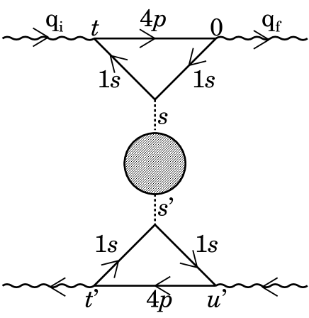
Figure 7: Diagrams for the RIXS intensity within the Born approximation to the $1s$ core-hole potential. The dotted lines represent the core-hole potential $V$. The shaded part represents the Keldysh-type Green’s function, which connects the outward time leg on the top half and the backward time leg on the bottom half.

The product of Green’s functions for the $4p$ electron and for the core hole, which are represented by lines with labels “4p” and “1s” in the figure, gives simply a factor $\exp[i(\epsilon_{4p}^{\eta}({\bf p})-\epsilon_{1s}-i\Gamma_{1s}-\omega_{i})t]$ on the outward time leg and a factor $\exp[-i(\epsilon_{4p}^{\eta}({\bf p})-\epsilon_{1s}+i\Gamma_{1s}-\omega_{i})(t^{\prime}-u^{\prime})]$ on the backward time leg, where $\Gamma_{1s}$ is a lifetime broadening width of the $1s$ core hole. The Keldysh Green’s function carries the time dependent factor ${\rm e}^{i\omega s}$ to the outward time leg and ${\rm e}^{-i\omega s^{\prime}}$ to the backward time leg. Note that the core-hole potential works only in intervals $[t,0]$ and $[t^{\prime},u^{\prime}]$. Integrating the time factor combined to the above product of Green’s functions, with respect to $s$ and $t$ in the region of $t<s<0$, $-\infty<t<0$, we obtain

$$L_{B}^{\eta}(\omega_{i};\omega) \equiv V\int_{-\infty}^{0}{\rm d}t\sum_{{\bf p}}\exp[i(\epsilon_{4p}^{\eta}({\bf p})-\epsilon_{1s}-i\Gamma_{1s}-\omega_{i})t]\int_{t}^{0}{\rm d}s\,{\rm e}^{i\omega s}$$ (21)

$$= \int\frac{V\rho_{4p}^{\eta}(\epsilon){\rm d}\epsilon}{(\omega_{i}+\epsilon_{1s}+i\Gamma_{1s}-\epsilon)(\omega_{i}-\omega+\epsilon_{1s}+i\Gamma_{1s}-\epsilon)}.$$

Here the sum over $4p$ states is replaced by the integration of the $4p$ DOS projected onto the $\eta$ ($=x,y,z$) symmetry, $\rho_{4p}^{\eta}(\epsilon)$. A similar factor has been derived in third-order perturbation theory by Abbamonte et al.Abbamonte et al. (1999) The integration with respect to $s^{\prime}$ and $t^{\prime}$ in the backward time leg gives the term complex-conjugate to Eq. (21). The integration with respect to $u^{\prime}$ give the energy conservation factor, which guarantees that $\omega$ in Eq. (21) is the energy loss, $\omega=\omega_{i}-\omega_{f}$. Finally, combining these relations together, we obtain an expression of the RIXS intensity for the incident photon with the momentum and energy $q_{i}=({\bf q}_{i},\omega_{i})$, polarization ${\bf{\rm e}^{(\alpha_{i})}}$, and the scattered photon with the momentum and energy $q_{f}=({\bf q}_{f},\omega_{f})$, polarization ${\bf{\rm e}^{(\alpha_{f})}}$:

$$W(q_{i},\alpha_{i};q_{f},\alpha_{f})=2\pi\frac{|w|^{4}}{4\omega_{i}\omega_{f}}\sum_{\xi\xi^{\prime}}Y_{\xi\xi^{\prime}}^{+-}(q)\left|\sum_{\eta}e_{\eta}^{(\alpha)}L_{B}^{\eta}(\omega_{i};\omega)e_{\eta}^{(\alpha^{\prime})}\right|^{2}.$$ (22)

Here $q=({\bf q},\omega)$ with ${\bf q}={\bf q}_{i}-{\bf q}_{f}$, $\omega=\omega_{i}-\omega_{f}$. Suffix $\xi$ and $\xi^{\prime}$ represent the $3d$ states distinguishing the A or B Ni sites.

III.2 The correlation function

We consider diagrams where one electron-hole pair remains after the RIXS process, as shown in Fig. 8(a). We write $Y_{\xi^{\prime},\xi}^{+-}(q)$ in the form,

$$Y_{\xi^{\prime},\xi}^{+-}(q)=\sum_{\xi_{1}\xi_{2}\xi_{3}\xi_{4}}\Lambda_{\xi_{1}\xi_{2},\xi^{\prime}}^{*}(q)\Pi_{\xi_{1}\xi_{2},\xi_{3}\xi_{4}}^{+-(0)}(q)\Lambda_{\xi_{3}\xi_{4},\xi}(q),$$ (23)

with

$$\Pi_{\xi_{1}\xi_{2},\xi_{3}\xi_{4}}^{+-(0)}({\bf q},\omega) = 2\pi\frac{2}{N}\sum_{{\bf k}}\sum_{j,j^{\prime}}\delta(\omega-E_{j^{\prime}}({\bf k+q})+E_{j}({\bf k}))[1-n_{j^{\prime}}({\bf k+q})]n_{j}({\bf k})$$ (24)

$$\times U_{\xi_{1}j^{\prime}}({\bf k+q})U_{\xi_{3}j^{\prime}}^{*}({\bf k+q})U_{\xi_{4}j}({\bf k})U_{\xi_{2}j}^{*}({\bf k}),$$

where $j$ and $j^{\prime}$ denote energy eigenstates. The $\delta$-function in $\Pi^{+-(0)}(q)$ indicates that the inter band transition from the valence band to the conduction band gives rise to the RIXS intensity. Only the weight of $3d$ states in the bands contributes to the intensity. We evaluate the vertex function in Eq. (23) within the RPA. Collecting the ladder diagrams shown in Fig. 8(b), we obtain

$$\Lambda_{\xi_{1}\xi_{2},\xi}(q)=\left[\hat{I}-\hat{\Gamma}\hat{F}^{--}(q)\right]_{\xi_{1}\xi_{2},\xi\xi}^{-1},$$ (25)

where $\hat{F}^{--}(q)$ is the conventional time-ordered propagator given by

$$[\hat{F}^{--}(q)]_{\xi_{1}\xi_{2},\xi_{3}\xi_{4}} = -i\frac{2}{N}\sum_{{\bf k}}\int\frac{{\rm d}k_{0}}{2\pi}G_{\xi_{4}\xi_{2}}({\bf k},k_{0})G_{\xi_{1}\xi_{3}}({\bf k+q},k_{0}+\omega)$$ (26)

$$= \frac{2}{N}\sum_{{\bf k}}U_{\xi_{4}j}({\bf k})U_{\xi_{2}j}^{*}({\bf k})U_{\xi_{1}j^{\prime}}({\bf k+q})U_{\xi_{3}j^{\prime}}^{*}({\bf k+q})$$

$$\times \left[\frac{n_{j}({\bf k})[1-n_{j^{\prime}}({\bf k+q})]}{\omega-E_{j^{\prime}}({\bf k+q})+E_{j}({\bf k})+i\delta}-\frac{n_{j^{\prime}}({\bf k+q})[1-n_{j}({\bf k})]}{\omega-E_{j^{\prime}}({\bf k+q})+E_{j}({\bf k})-i\delta}\right].$$

The four-point vertex is non-zero only for $\xi_{1}$, $\xi_{2}$, $\xi_{3}$, $\xi_{4}$ belonging to the same Ni site, that is,

$$[\hat{\Gamma}]_{\xi_{1}\xi_{2},\xi_{3}\xi_{4}}=\Gamma^{(0)}(\xi_{1}\xi_{4};\xi_{2}\xi_{3}),$$ (27)

and otherwise it is zero.

Figure 8: (a)Diagrams for $Y^{+-}(q)$. Solid lines with arrows are not the time-ordered Green’s functions but the Keldysh-type ones connecting the outward time leg with the backward time leg. (b)Vertex function $\Lambda(q)$ within the RPA. Solid lines with arrows are the conventional time-ordered Green’s functions. The square represents the four-point vertex of the $3d$ Coulomb interaction effective only at the same Ni sites. (c)Diagrams for the time-ordered $Y^{{\rm T}}(q)$ within the RPA.

As already pointed out, the Keldysh-type Green’s function $Y_{\xi^{\prime},\xi}^{+-}(q)$ is equivalent to the conventional correlation function. Therefore, it may be more convenient to analyze the function with the help of the conventional time-ordered Green’s function,

$$Y_{\xi^{\prime},\xi}^{{\rm T}}({\bf q},t)=-i\langle T[\rho_{{\bf q}m^{\prime}\sigma^{\prime}}^{\lambda^{\prime}}(t)(\rho_{{\bf q}m\sigma}^{\lambda})^{\dagger}(0)]\rangle,$$ (28)

with $T$ being the time-ordering operator. Considering the diagrams shown in Figs. 8(b) and (c), it is expressed within the RPA as

$$Y_{\xi^{\prime},\xi}^{{\rm T}}(q)=\left\{\hat{F}^{--}(q)[\hat{I}-\hat{\Gamma}\hat{F}^{--}(q)]^{-1}\right\}_{\xi^{\prime}\xi^{\prime},\xi\xi}.$$ (29)

This expression leads to Eq. (23) with the help of the fluctuation-dissipation theorem (FDT),

$$\sum_{\xi^{\prime}\xi}Y_{\xi^{\prime}\xi}^{+-}(q)=-i\sum_{\xi^{\prime}\xi}\left[Y_{\xi^{\prime}\xi}^{{\rm T}*}(q)-Y_{\xi\xi^{\prime}}^{{\rm T}}(q)\right]\quad{\rm for}\,\,\omega>0.$$ (30)

To show this fact, we first rewrite Eq. (26) as

$$\hat{F}^{--}(q)=\hat{F}_{1}^{--}(q)+i\hat{F}_{2}^{--}(q),$$ (31)

where $\hat{F}_{1}^{--}(q)$ and $\hat{F}_{2}^{--}(q)$ are Hermitian matrices. Then, using the Hermitian property, we transform $Y_{\xi^{\prime}\xi}^{{\rm T}}(q)^{*}$ as

$$Y_{\xi^{\prime}\xi}^{{\rm T}}(q)^{*} = \bigl{\{}[I-(F_{1}^{--}(q)-iF_{2}^{--}(q))\Gamma]^{-1}[F_{1}^{--}(q)-iF_{2}^{--}(q)]$$ (32)

$$\times [I-\Gamma(F_{1}^{--}(q)+iF_{2}^{--}(q))][I-\Gamma(F_{1}^{--}(q)+iF_{2}^{--}(q))]^{-1}\bigl{\}}_{\xi\xi^{\prime}}.$$

Combining the similar expression for $Y_{\xi\xi^{\prime}}^{{\rm T}}(q)$, we have

$$Y_{\xi^{\prime}\xi}^{{\rm T}*}(q)-Y_{\xi\xi^{\prime}}^{{\rm T}}(q)=\bigl{\{}[I-(F_{1}^{--}(q)-iF_{2}^{--}(q))\Gamma]^{-1}(-2i)[\hat{F}_{2}^{--}(q)][I-\Gamma(F_{1}^{--}(q)+iF_{2}^{--}(q))]^{-1}\bigl{\}}_{\xi\xi^{\prime}}.$$ (33)

Since $-2F_{2}^{--}(q)$ is equivalent to $\Pi^{(0)}(q)$ for $\omega>0$, the RXS intensity given by Eq. (33) through Eq. (30) is equivalent to the one given by Eq. (23).

Equation (29) has sometimes poles for some frequencies below the energy continuum of an electron-hole pair. These bound states may be called as “$d$-$d$ excitations”, and give rise to extra RIXS peaks. To analyze the problem, we rewrite Eq. (29) as

$$Y_{\xi^{\prime},\xi}^{{\rm T}}(q)=\left[\hat{F}^{--}(q)^{-1}-\hat{\Gamma}\right]_{\xi^{\prime}\xi^{\prime},\xi\xi}^{-1},$$ (34)

where ${\hat{F}}^{--}(q)^{-1}$ becomes an Hermitian matrix for $\omega$ below the energy continuum. Therefore, ${\hat{F}}^{--}(q)^{-1}-\Gamma$ can be diagonalized by a unitary matrix. Let the diagonalized matrix have a zero component at $\omega=\omega_{B}({\bf q})$ with the corresponding eigenvector $B_{\xi_{1}\xi_{2}}({\bf q})$. Then, $Y_{\xi^{\prime}\xi}^{{\rm T}}(q)$ can be expanded around $\omega\sim\omega_{B}({\bf q})$ as

$$Y_{\xi^{\prime}\xi}^{{\rm T}}(q)=\frac{C_{\xi^{\prime}\xi}({\bf q})}{\omega-\omega_{B}({\bf q})},$$ (35)

with

$$C_{\xi^{\prime}\xi}({\bf q})=\frac{B_{\xi^{\prime}\xi^{\prime}}({\bf q})B_{\xi\xi}^{*}({\bf q})}{\sum_{\xi_{1}\xi_{2}\xi_{3}\xi_{4}}B_{\xi_{1}\xi_{2}}^{*}({\bf q})\frac{\partial}{\partial\omega}[\hat{F}^{--}(q)^{-1}]_{\xi_{1}\xi_{2},\xi_{3}\xi_{4}}B_{\xi_{3}\xi_{4}}({\bf q})}.$$ (36)

Substituting the right hand side of Eq. (30) by this equation, we obtain

$$\sum_{\xi^{\prime}\xi}Y_{\xi^{\prime}\xi}^{+-}(q)=2\pi\sum_{\xi^{\prime}\xi}C_{\xi^{\prime}\xi}(q)\delta(\omega-\omega_{B}({\bf q})).$$ (37)

This relation is to be inserted into Eq. (22) for evaluating the RIXS spectra.

IV Calculated Results

We calculate the RIXS intensity from Eq. (22). The $\delta$-function in $Y^{+-}(q)$ is replaced by the Lorentzian function with the FWHM $=0.2$ eV in order to take account of the instrumental resolution. Corresponding to the experimental situation that the polarization of photon is not specified, we use the realistic $4p$-DOS in evaluating $L_{B}^{\eta}(\omega_{i};\omega)$ (Eq. (21)) and tune the incident photon energy on the top of the $4p$-DOS. Figure 9 shows the calculated spectra as a function of energy loss in comparison with the experiment by Ishii et al.Ishii The momentum transfer is chosen along symmetry axes in the Brillouin zone.

Figure 9: RIXS spectra as a function of energy loss $\omega=\omega_{i}-\omega_{f}$, in comparison with the experiment by Ishii et al.Ishii Momentum transfer is along the symmetry lines: (a) $\Gamma$- $\frac{2\pi}{a}(0.25,0.25,0.25)$-$L$, (b) $\Gamma$-$\frac{2\pi}{a}(0.3,0,0)$-$X$, and (c) $\Gamma$-$\frac{2\pi}{a}(0.25,0.25,0)$-$K$. The incident photon energy is tuned to excite the $1s$ electron to the peak of the $4p$-DOS. The broken and solid lines are the results of the HFA and RPA, respectively. The dotted lines represent the experimental data.Ishii

The spectra arise from the excitation from the valence states with the $e_{g}$ character to the conduction states with also the $e_{g}$ character. Since the unoccupied states are almost concentrated in the minority spin states (see Fig. 6), the electron-hole pair creation occurs in the minority spin channel. They form a continuum spectrum. Several peaks are already present within the HFA. Some peaks are suppressed and some are enhanced by the RPA. At the $\Gamma$ point, peaks are found around 4-6 eV and around 8 eV, in good agreement with the experiment. In addition, an extra peak is found around the upper edge of the continuum, $\sim 10$ eV, which is not confirmed by the experiment (the observation is limited below 10 eV). With momenta deviating from the $\Gamma$ point, intensities around 5-6 eV is particularly enhanced in the entire region of 4-6 eV. Thereby the spectral shape looks like the peak position is moving with changing momenta. On the other hand, the peak around 8 eV does not change its position with changing momenta. These characteristics are the same along the three symmetry lines. The spectral shapes show excellent agreement with the experiment. Ishii Note that the sharp peak around 10 eV is strongly suppressed with deviating momenta from the $\Gamma$ point.

Below the lower edge of the continuum spectra, we obtain a bound state at 2 eV, as shown in Fig. 10. This may be compared with the experimental peak at 1.7 eV, but the calculated intensity is about two order of magnitude smaller. At present, we do not know the real origin for this discrepancy.

Figure 10: RIXS intensity below the lower edge of the continuum at $\Gamma$ point in comparison with the experiment. Ishii The calculated intensity is enlarged by multiplying 200 to make the spectra visible.

V Concluding Remarks

We have analyzed the RIXS spectra in NiO by developing the formalism of Nomura and Igarashi. This is based on the Keldysh Green’s function formalism and relates the RIXS spectra to the density-density correlation function under the Born approximation to the core-hole potential. The use of the Born approximation had been justified for the RIXS in La₂CuO₄ by evaluating the multiple scattering effects.Igarashi et al. Since NiO has a larger energy gap than La₂CuO₄, we expect that the Born approximation is better justified in NiO. We have introduced the tight-binding model including all the Ni $3d$ and O $2p$ orbitals as well as the full Coulomb interaction between $3d$ orbitals, and have calculated the single-particle excitation within the HFA. The RIXS spectra are generated by the band-to-band transition to screen the $1s$ core hole. We have calculated the RIXS spectra using the single-particle band thus evaluated together with the $4p$ DOS by the LDA. The electron correlation is treated within the RPA. We have obtained several peaks in the continuum spectra. Two peaks are found prominent around 5 eV and 8 eV, and the one around 5 eV shifts to the higher energy position while another around 8 eV does not move with momenta changing to the zone boundary. The calculated spectral shape show quantitative agreement with the experiment. The excellent agreement with the experiment suggests that the present scheme is useful to analyze the RIXS spectra. As regards the ”$d$-$d$” excitation, we have obtained a bound state below the lower edge of the continuum spectrum. However, the intensity is about two order of magnitude smaller than the experimental one. The presence of crystal distortion might enhance the intensity of ”$d$-$d$” excitation. At any rate, the real reason for this discrepancy is not known.