Disorder-induced magnetic memory: Experiments and theories

M. S. Pierce^1,2, C. R. Buechler¹, L. B. Sorensen¹, S. D. Kevan³, E. A. Jagla⁴, J. M. Deutsch⁵,T. Mai⁵, O. Narayan⁵, J. E. Davies⁶, Kai Liu⁶, G. T. Zimanyi⁶, H. G. Katzgraber⁷, O. Hellwig⁸, E. E. Fullerton⁸, P. Fischer⁹, and J. B. Kortright⁹ ¹Department of Physics, University of Washington, Seattle, Washington 98195, USA ²Materials Science Division, Argonne National Laboratory, Argonne Illinois 60439, USA ³Department of Physics, University of Oregon, Eugene, Oregon 97403, USA ⁴Centro Atómico Bariloche, Comisión Nacional de Energía Atómica, (8400) Bariloche, Argentina ⁵Department of Physics, University of California, Santa Cruz, California 95064, USA ⁶Department of Physics, University of California, Davis, California 95616, USA ⁷Theoretische Physik, ETH Zürich, CH-8093 Zürich, Switzerland ⁸Hitachi Global Storage Technologies, San Jose, California 95120, USA ⁹Lawrence Berkeley National Laboratory, Berkeley, California 94720, USA

Abstract

Beautiful theories of magnetic hysteresis based on random microscopic disorder have been developed over the past ten years. Our goal was to directly compare these theories with precise experiments. To do so, we first developed and then applied coherent x-ray speckle metrology to a series of thin multilayer perpendicular magnetic materials. To directly observe the effects of disorder, we deliberately introduced increasing degrees of disorder into our films. We used coherent x-rays, produced at the Advanced Light Source at Lawrence Berkeley National Laboratory, to generate highly speckled magnetic scattering patterns. The apparently “random” arrangement of the speckles is due to the exact configuration of the magnetic domains in the sample. In effect, each speckle pattern acts as a unique fingerprint for the magnetic domain configuration. Small changes in the domain structure change the speckles, and comparison of the different speckle patterns provides a quantitative determination of how much the domain structure has changed. Our experiments quickly answered one longstanding question: How is the magnetic domain configuration at one point on the major hysteresis loop related to the configurations at the same point on the loop during subsequent cycles? This is called microscopic return-point memory (RPM). We found the RPM is partial and imperfect in the disordered samples, and completely absent when the disorder was below a threshold level. We also introduced and answered a second important new question: How are the magnetic domains at one point on the major loop related to the domains at the complementary point, the inversion symmetric point on the loop, during the same and during subsequent cycles? This is called microscopic complementary-point memory (CPM). We found the CPM is also partial and imperfect in the disordered samples and completely absent when the disorder was not present. In addition, we found that the RPM is always a little larger than the CPM. We also studied the correlations between the domains within a single ascending or descending loop. This is called microscopic half-loop memory (HLM) and enabled us to measure the degree of change in the domain structure due to changes in the applied field. No existing theory was capable of reproducing our experimental results. So we developed new theoretical models that do fit our experiments. Our experimental and theoretical results set new benchmarks for future work.

pacs:

07.85.+n, 61.10.-i, 78.70.Dm, 78.70.Cr

I Introduction

What causes magnetic hysteresis and how is it induced and influenced by coexisting microscopic disorder? This is the question that we address and provide new answers about in this paper. We are able to provide new information about this venerable old question because we have developed a new way to directly probe the effect of disorder on the spatial structure of the microscopic magnetic domain configuration as a function of the applied magnetic field history. When we finished our experimental study, we discovered that our results could not be explained by any existing microscopic theories of magnetic hysteresis. So we developed several viable theoretical models. In this paper, we present our detailed experimental results and the theoretical models that we developed to explain them.

Magnetic hysteresis is fundamental to all magnetic storage technologies and consequently is a cornerstone of the present information age. The magnetic recording industry deliberately introduces carefully controlled disorder into its materials to obtain the desired hysteretic behavior and magnetic properties. Over the past 40 years, such magnetic hardening has developed into a high art form. However, despite decades of intense study and significant recent advances, we still do not have a completely satisfactory microscopic understanding of magnetic hysteresis.

The exponential growth of computing power that fueled the information age has been driven by two technological revolutions: 1) The integrated circuit revolution and its exponential growth described by Moore’s Law. 2) The magnetic disk drive revolution and its exponential growth which for the past decade has surpassed Moore’s Law. Both of these mature technologies are rapidly approaching their fundamental physical limits. If the incredible growth rate of storage capacity in magnetic media is to continue, new advances in our fundamental understanding of magnetic hysteresis are needed.

For the past 20 years, magnetic films with perpendicular anisotropy have been extensively studied for their potential to extend the limits of storage capacity. Early in 2005, the first commercial disk drives using perpendicular magnetic media became available. The system that we study here is a model for these new perpendicular magnetic media. In this paper, we present our results on the effect of disorder on the correlations between the domain configurations in these systems.

To study the detailed evolution of the magnetic domain configuration correlations in our samples, we developed a new x-ray scattering technique, coherent x-ray speckle metrology (CXSM). We illuminate our samples with coherent x-rays tuned to excite virtual 2p to 3d resonant transitions in cobalt. The resulting resonant excitation of the cobalt provides our magnetic signal. The coherence of the x-rays produces a magnetic x-ray speckle pattern. The positions and intensity of the speckles provides a detailed fingerprint of the microscopic magnetic domain configuration. Changes in the magnetic domain configuration produce changes in the speckle pattern. So by comparing these magnetic fingerprints versus the magnetic field history—by cross-correlating speckle patterns with different magnetic field histories—we obtain a quantitative measure of the applied field-history-induced evolution of the magnetic domain configuration.

Here we report our results obtained by applying CXSM to investigate the effects of controlled disorder on the magnetic domain evolution in a series of Co/Pt multilayer samples with perpendicular anisotropy. We introduced disorder into the samples by systematically increasing the interfacial roughness of the Co/Pt multilayers during the growth process. We found that this disorder induces memory in the microscopic magnetic domain configurations from one cycle of the hysteresis loop to the next, despite taking the samples through magnetic saturation. Our lowest disorder samples have no detectable cycle-to-cycle memory; their domain patterns are unique each time the sample is cycled around the major loop. As we increase the disorder, the cycle-to-cycle memory develops and grows to a maximum value, but never becomes perfect or complete at room temperature.

In this paper, we only present our results for microscopic magnetic memory along the major loop in the slow field sweep limit. In this limit, the measured hysteresis loop is the same over many decades of sweep rate. The hysteresis in this limit is often called rate-independent hysteresis, or quasi-static hysteresis. There are, of course, also interesting and important hysteresis effects that occur at high sweep rates. Our strategy was to study the simpler rate-independent hysteresis case before adding the additional physics, and complications, associated with high sweep rates. As we explain below, the disorder dependence of the rate-independent hysteresis in our system turned out to be remarkably rich and interesting. We do not discuss our results for rate-independent minor loop memory in this paper, but we briefly reported them recently prl1 .

The best modern microscopic disorder-based theories of magnetic hysteresis were built on the foundations of Barkhausen noise measurements sethna-dahmen . Even in the rate-independent limit, the magnetization of a disordered ferromagnet does not change smoothly as the applied field is swept up and down. Instead, there are magnetic domain avalanches that produce magnetization jumps. These avalanches exhibit power-law size distributions indicating that many different size regions change their magnetization in jumps as the field is swept around the major hysteresis loop.

A comprehensive, recent review of Barkhausen noise studies—including a translation of Barkhausen’s 1919 paper—is given in Ref. zapperi . For some materials in the rate-independent limit, the Barkhausen noise is independent of the magnetic sweep rate; these avalanches occur at fixed values of the applied field, independent of the sweep rate zapperi_prl .

Barkhausen measurements provide exquisite information about the time structure of the avalanches, but they usually do not provide any spatial information about the location of the avalanches. Because we directly measure the nanometer scale spatial structure of the magnetic domain configuration changes, we obtain detailed information about the configuration evolution that cannot be obtained directly from the best classical Barkhausen noise studies or from their modern optical implementations optical-bark . Because there has been extensive theoretical work on Barkhausen noise, the corresponding field-history-dependent microscopic morphologies of the magnetic domain configurations have been indirectly inferred from the Barkhausen time-signals via detailed computer simulations. For example, Sethna, Dahmen and their co-workers have shown that the morphology for their random field Ising model (RFIM) is fractal in space. They provide a comprehensive review of their work in Ref. sethna-dahmen .

Taken together, the detailed fractal-in-time structure measured via the Barkhausen noise, and the extensive computer simulations by Sethna, Dahmen, and others, imply that their magnetic domain configurations are fractal in space. Therefore, why not simply measure the correlations between the magnetic domain configurations directly? That is precisely what we do in this paper. There has been very little systematic, ensemble-level experimental work on the spatial evolution of the magnetic domain configurations optical-bark ; waveform_magnetics , but this information is readily available from the existing simulations. However, up until now almost all of the work has been done for pure RFIMs. Our experimental system and the new generation of perpendicular magnetic disk drive media have long-range dipole interactions. This means that new theories that include the dipolar interactionsdipolar_rmp will be required to understand these materials.

During our work, we unearthed three interesting aspects of our magnetic domain wall evolution. The first, called major loop return-point memory (RPM), describes the magnetization for each point on the major loop. If this magnetization is precisely the same for each cycle around the major loop, then we have macroscopic major loop RPM. If, in addition, the microscopic magnetic domain configuration is also identical, then we have microscopic major loop RPM. Our experiments show that our samples have perfect macroscopic major loop RPM, but imperfect microscopic major loop RPM at room temperature.

The second, called complementary-point memory (CPM), describes the inversion symmetry of the major loop through the origin. If the magnetization at field $H$ on the descending branch is equal to the minus the magnetization at field $-H$ on the ascending branch, then we have perfect macroscopic major loop CPM. If, in addition, the magnetic domains are precisely reversed, then we have perfect microscopic major loop CPM. Our experiments show that our samples have perfect macroscopic major loop CPM, but imperfect microscopic major loop CPM at room temperature. In addition, we find that our measured values for the microscopic RPM are consistently a little larger than those for our microscopic CPM—thus the RPM-CPM symmetry is slightly broken.

The third, called half-loop-memory(HLM), describes the degree of change in the magnetic domain configurations along a single branch of the major hysteresis loop. Our experiments show that disorder has a direct effect on how the domains evolve. The greater the disorder present in the sample, then the greater the observed changes in the domain configurations as the applied field is slowly adjusted to take the system along the major hysteresis loop. Our measured values for the HLM are consistently higher in the low disorder samples than those present in the disordered samples.

We were inspired to do our experimental study by the beautiful work on the RFIM by Sethna, Dahmen, and coworkers sethna-dahmen . We were therefore very surprised to discover that their model could not describe our experimental results. Their pure zero-temperature RFIM predicts perfect macroscopic and microscopic major loop RPM, but it does not agree with our experiments because it predicts essentially no microscopic major loop CPM. It seems reasonable that their $T>0$ RFIM will predict perfect macroscopic RPM but imperfect microscopic RPM like that observed in our experiments, but this has not been tested. However their model cannot predict our observed microscopic CPM and therefore it also cannot predict the slightly broken microscopic RPM-CPM symmetry that our experiments observe.

So, what physics is required to produce imperfect microscopic RPM and CPM with the slightly broken symmetry? There are two aspects to this question—the imperfection and the RPM-CPM symmetry breaking. Almost all models have perfect memory at $T=0$ and imperfect memory for $T>0$ . And it seems likely that the imperfect memory that we observe could be caused by temperature effects, but this has not yet been established. On the other hand, no viable theoretical model for the slight RPM-CPM symmetry breaking existed. So we developed viable models. The key idea behind each of our models was to combine physics with spin-reversal symmetry with physics without spin-reversal symmetry. Then the spin-reversal-symmetric physics produces symmetric memory ${{\rm RPM}={\rm CPM}}$ and the non-symmetric physics produces symmetry-broken memory ${{\rm RPM}\not={\rm CPM}}$ .

Within the standard RXIM models—viz., RAIM, RBIM, and RCIM, and RFIM where A denotes anisotropy, B denotes bond, C denotes coercivity, and F denotes field—the first three have spin-reversal symmetry, but the fourth (RFIM) does not. So one way to produce slightly symmetry-broken memory is to combine the RFIM with one of the symmetric models. Surprisingly, another way is to combine one of the symmetric models with vector spin dynamics because vector dynamics breaks the spin-reversal symmetry. We report our work on three viable models: Model 1 combines a pure RFIM with a pure RCIM. Model 2 combines a pure RAIM with vector spin dynamics. Model 3 combines a pure RFIM with a pure spin-glass model

We explored Model 1 and Model 2 in the most detail. By tuning the model parameters, we were able to semi-quantitatively match our experimentally observed disorder-dependence and magnetic-field-dependence of (i) the domain configurations, (ii) the shape of the major loops, (iii) the values of the RPM and CPM, and (iv) the slight RPM-CPM symmetry breaking.

Note that in order to properly describe our observed magnetic domain configurations, we had to include the long-range dipolar interactions. In contrast to the Sethna-Dahmen RFIMs that predict spatially fractal magnetic domain configurations sethna-dahmen , our samples exhibit labyrinthine domain configurations due to their long-range dipolar interactions.

The remainder of this paper is organized as follows. Section 2 describes the physics of return point memory and complementary point memory. Section 3 describes our experiments, sample fabrication, structural characterization, magnetic characterization, and coherent x-ray speckle metrology (CXSM) characterization. Section 4 describes our data analysis methodology. Section 5 describes the results of our data analysis. Section 6 describes the theoretical models that we developed to account for the observed behavior of our system. Section 7 presents our conclusions.

II Macroscopic and Microscopic Return-Point Memory and Complementary Point Memory

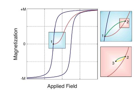
In his 1903 dissertation at Göttingen entitled “On the magnetization produced by fast currents and the operation of Rutherford-Marconi magnetodetectors,” Erwin Madelung presented his rules for magnetic hysteresis as illustrated in Figure 1:

1.

Major-loop return-point memory.

The magnetization of the sample at every point on the major loop is completely determined only by the applied field, and all first-order reversal curves starting from the major loop and going to saturation are uniquely determined by their starting point. The curve $1\rightarrow+S$ in Fig. 1 illustrates a first-order reversal curve (forc).
2.

Minor-loop return-point memory.

The magnetization of the sample at every point on the major loop is completely determined solely by the value of the applied field, even when the point on the major loop is reached starting from a point inside the major loop. This holds for every order reversal curve. The curve $2\rightarrow 1$ illustrates this property for a second-order reversal curve (sorc).
3.

The memory deletion property, a.k.a. the wiping out property.

The magnetization of the sample at every point on a reversal curve is precisely the same as that for its parent curve as soon the reversal curve returns to its parent. In this way, all memory of the previous field history between the initial departure from the parent and the return to the parent has been erased. This holds for every order reversal curve. The curve $3\rightarrow+S$ illustrates this for a third-order reversal curve (torc).
4.

The congruency property.

All return curves that start from reversal at the same value of the applied field have the same shape thereafter independent of the entire previous applied field history.
5.

The similarity property for initial magnetization curves.

When any initial magnetization curve is reversed at point a, the reversed return curve to saturation will pass through the inversion symmetric point to a as it proceeds to saturation. As discussed below, we call the analogous property to the similarity property—for reversal curves that do not start from a point on the initial magnetization curve—the complementary-point memory property.

Madelung formulated his rules based on his careful experimental studies of different alloys of steel and published them in 1905 and 1912 madelung_05 . Because Madelung formulated his rules before the existence of magnetic domains was known, he only considered the macroscopic magnetization. Nevertheless, his rules still predict the macroscopic magnetization of “any typical” sample versus its applied field history. Madelung’s rules have truly been the foundation for all modern theories of hysteresis.

It is therefore surprising that Madelung’s rules are so rarely cited. Apparently this is because essentially all of the subsequent work has been focused on the Preisach model. The obscurity of Madelung’s magnetic hysteresis work is particularly surprising because the Preisach model has been well known to be unphysical for a very long time due to heavy reliance on phenomenology.

Of course, Madelung’s rules do not apply to every magnetic system. For example, many systems exhibit accomodation, reptation and magnetic viscosity effects, and all systems exhibit dynamic hysteresis effects. However, on the other hand, Madelung’s rules do apply to an incredible number of magnetic systems under a vast range of conditions.

Now that we know that the microscopic magnetic domains are intimately involved in the production of magnetic hysteresis, we immediately come to the first question at the core of our investigation: How do the magnetic domains behave on the microscopic level. Do the domains remember—viz., return precisely to—their initial states, or does just the ensemble average remember? We show below that, at room temperature, some of the domains in our samples return to their original configurations and some do not, but nevertheless the macroscopic magnetization—set by the ensemble average—does return to its original value.

In other words, we find that our samples have perfect macroscopic RPM, but they have imperfect microscopic RPM at room temperature. In fact, our measured RPM values for each sample demonstrate a rich, complex behavior reflecting the fundamental physics of the magnetic domains. We quantitatively measured the fraction of the domains that remember and thereby demonstrated that the disorder has a profound impact on the microscopic RPM. As we tune the disorder, our samples develop microscopic RPM that starts from zero in the low-disorder limit and jumps to a saturated value in the high-disorder limit, but never becomes perfect at room temperature. Consequently, our experimental system is a finite-temperature realization of the “microscopic disorder-induced phase transition between no memory and perfect memory” predicted by Sethan, Dahmen, and coworkers sethna-dahmen .

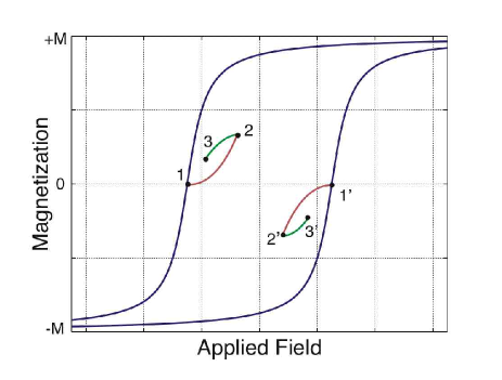
The major loop for “any typical” magnetic system usually has an additional symmetry—it is symmetric about inversion through the origin. This inversion symmetry immediately raises the second question at the core of our investigation: How are the domains at the complementary points of the major loop related? Do the magnetic domains at the opposing points on the major loop evolve in a similar, but perhaps mirror correlated fashion? We call this effect microscopic major loop CPM. The geometry of complementary-point memory is illustrated in Fig. 2.

Despite an incredible amount of effort since 1905, it has proven impossible to develop a simple, yet adequate, phenomenological model that can be used to treat all magnetic materials. We still do not have a phenomenological model for modern magnetic technology. In addition, although there has also been tremendous effort expended and progress achieved, it has similarly proven impossible to develop a general purpose micromagnetics model. We now know, based on recent theoretical work sethna-dahmen , that the detailed magnetic hysteresis properties of real materials cannot be treated using standard mean-field methods. This is because the hysteresis depends on the interactions between each domain and a limited number of its neighbors, as well as between each domain and its local disorder. Consequently, our approach has been to determine to what extent the nanoscale domain-level physics of our experimental system obeys Madelung’s rules, and then to explore whether we can better understand the observed behavior using traditional (overly) simplified Ising models.

Refer to caption — Figure 1: The topology of Madelung’s rules. (a) If the magnetization curves from point 1 to saturation are uniquely determined by the applied field at their departure point 1 from the major loop, then the system exhibits macroscopic major-loop return-point memory. If after returning to point 1 on the major hysteresis loop, the system continues along the major loop, then the system exhibits macroscopic major-loop memory deletion (wiping out). (b) If the first-order reversal curve from point 2 back to the major loop arrives at its original departure point, then the system exhibits first-order macroscopic minor-loop return-point memory. (c) If the second-order reversal curve from point 3 back towards saturation passes through point 2, then the system exhibits second-order macroscopic minor-loop return-point memory. If thereafter it continues along the original curve from 1 to saturation, then the system exhibits macroscopic minor-loop memory deletion (wiping out).

III Experimental Aspects

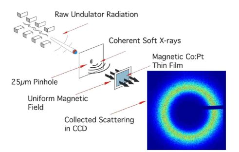
To measure the field-history induced changes in the microscopic magnetic domain configurations, we developed coherent x-ray speckle metrology (CXSM) prl1 ; prl2 ; srn . Our CXSM experiments were performed at the Advanced Light Source at Lawrence Berkeley National Laboratory. A schematic diagram of the experimental apparatus is shown in Figure 3. We used linearly polarized x-rays from the third and higher harmonics of the beamline 9 undulator. The raw undulator beam was first reflected from a nickel-coated-bremmstrahlung-safety mirror and then passed through a water-cooled Be window to decrease unwanted light. The partially coherent incident beam from the undulator was passed through a 35-micron-diameter pinhole to select a transversely coherent portion. The sample was located 40 centimeters downstream of the coherence-selection pinhole. This provided transversely coherent illumination of about a 40 micron diameter area of the sample. The transversely coherent x-ray beam was incident perpendicular to the sample surface and was scattered in transmission by the sample. The resonant magnetic scattering was detected by a soft x-ray CCD camera located 1.1 meters downstream of the sample. Between the sample and the CCD camera we used a small blocker to prevent the direct beam from damaging the CCD.

The photon energy was set to the cobalt L3 resonance at $778$ eV. These photons resonantly excited virtual 2p to 3d transitions in the cobalt atoms and thereby provided our magnetic sensitivity. The intensity of the raw undulator beam was $2\times 10^{14}$ photons/sec, the intensity of the coherent beam was $2\times 10^{12}$ photons/sec, and the intensity of the scattered beam was $2\times 10^{7}$ photons/sec. We typically measured each speckle pattern for 10 to 100 seconds, so the total number of photons in each CCD image was $10^{8}$ to $10^{9}$ .

The applied magnetic field was provided by an in-vacuum water-cooled electromagnet allowing in situ adjustment of the magnetic field during the experiment. The return path for the electromagnet consists of an external soft Fe yoke that feeds field to vanadium permandur pole pieces that are integral to the vacuum chamber. The pressure inside the chamber during our experiments was typically $10^{-8}$ Torr. The in-vacuum electromagnet provided magnetic fields up to $11$ kOe.

III.1 Sample Fabrication and Structural Characterization

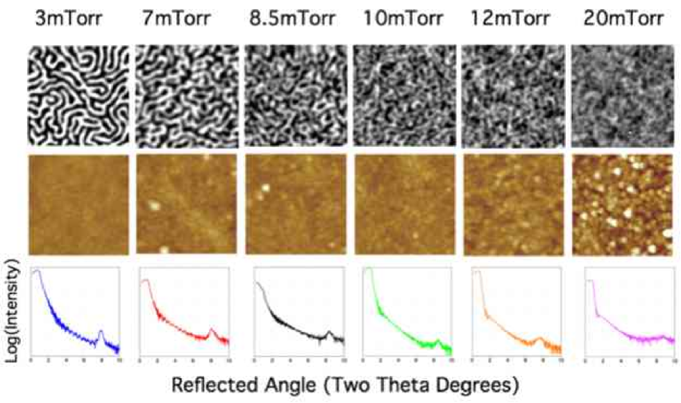
Our thin-film samples were grown by magnetron sputtering in the San Jose Hitachi Global Storage Technology Laboratory on smooth, low-stress, 160-nm-thick silicon nitride membranes. The samples had 20-nm-thick Pt buffer layers, and 2.3-nm-thick Pt caps to prevent oxidation. Between the buffer layer and the cap, the samples had 50 repeating units of a 0.4-nm-thick Co layer and a 0.7-nm-thick Pt layer. While the six samples had identical multilayer structure they were grown at different argon sputtering pressures to tune the disorder in the samples. During growth, we adjusted the deposition times to keep the Co and Pt layer thickness constant over the entire series. For low argon pressures, the sputtered metal atoms arrive at the growth substrate with considerable kinetic energy which locally heats and anneals the growing film. This leads to smooth Co/Pt interfaces produced at a low sputtering pressure. For higher argon sputtering pressures, the sputtered atoms arrive at the growth substrate with minimal kinetic energy thereby resulting in rougher Co/Pt interfaces. The resulting roughness is cumulative through the samples eric-prb . The magnetocrystaline anisotropy at the Co/Pt interface forces the magnetization to align perpendicularly to the surface of the film. Our samples were grown at six different sputtering pressures: 3, 7, 8.5, 10, 12, and 20 mTorr. Due to the important and interesting magnetic properties, these samples and others very similar in form and structure have been studied in different experimentsolav_physicab ; davies .

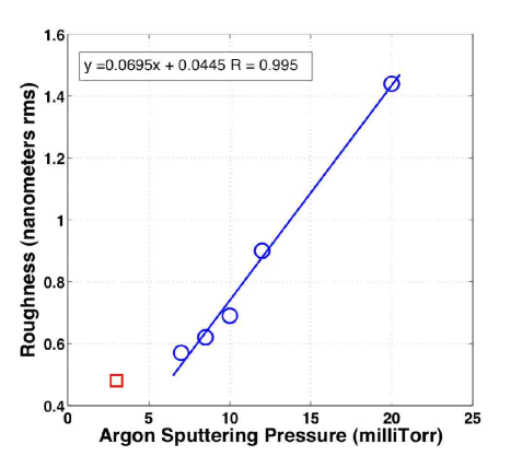
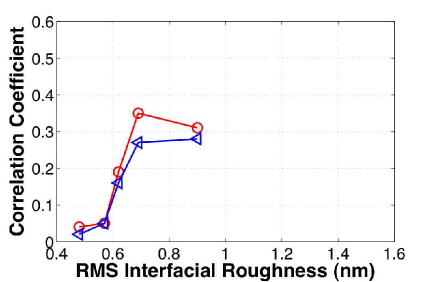
The rms roughness for the samples was measured in the Almaden Hitachi Global Storage Technology Laboratory using two different methods. First, we measured the roughness by scanning the sample surface with an atomic force microscope (AFM) and calculating the rms roughness from the AFM images. Since our samples have conformal roughness, the rms roughness of the surface is a reasonable measure of the internal rms roughness. However, to directly probe the internal rms roughness, we also did the x-ray reflectivity measurements shown in Fig. 5. The reflectivity data was fit using a Debye-Waller factor to determine the roughness. Instead of the system possessing thermal fluctuations, the displacements from the average height are randomly distributed and fixed. The rms roughness values from the x-ray measurements agreed with those from the AFM measurements, confirming the conformal roughness of our samples. The rms roughness values are shown in Fig. 4 and are listed in Table 1. We found that the rms roughness for the 3 mTorr sample is about 0.48 nm and that it increases to 1.44 nm for the 20 mTorr sample.

III.2 Magnetic Characterization

Table 1: The Measured Magnetic Characteristics of Our Six Samples

Sample¹¹1Our samples are labeled by their growth pressure in mTorr	$\sigma_{{\it{rms}}}$ ²²2The measured rms interfacial roughness in nm	$M_{s}$ ³³3The measured saturation magnetization of Co in $emu/cm^{3}$	$H_{n}$ ⁴⁴4The nucleation field measured from positive saturation	$H_{c}$ ⁵⁵5The measured coercive field in kOe	$H_{s}$ ⁶⁶6The measured saturation field in kOe
3 mTorr	0.48	1360	1.58	0.16	3.7
7 mTorr	0.57	1392	0.64	0.68	5.0
8.5 mTorr	0.62	1136	1.68	1.42	5.5
10 mTorr	0.69	1069	1.45	1.87	6.5
12 mTorr	0.90	1101	1.23	2.74	9.5
20 mTorr	1.44	918	-1.81	5.89	14.2

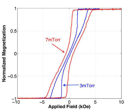
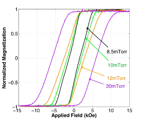
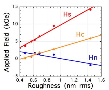
We measured the major hysteresis loops for all of our samples using both Kerr magnetometry at the San Jose Hitachi Global Storage Technology Laboratory and alternating gradient magnetometry (AGM) at the University of California-Davis. The measured major loops shown in Fig. 6 exhibit clear changes that are related to the increasing roughness. The two low disorder films (3 mTorr and 7 mTorr) exhibited “classic Kooy-Enz kooy-enz soft loops” with low remanence and abrupt nucleation transitions. Between 7 mTorr and 8.5 mTorr, there is an abrupt transition to loops which do not show a clear nucleation region. Between 8.5 mTorr and 20 mTorr, the ascending and descending slopes of the loop remain the approximately the same, but the loops gradually widen until the full magnetic moment is left at remanence. The values of the nucleation, coercive and saturation fields each exhibit a roughly linear dependence upon the sample roughness. This behavior is shown in Fig. 7. In addition, we also found via magnetometry that all of our films exhibit perfect macroscopic major loop and minor loop RPM and CPM.

The AGM magnetometer was used to measure the saturation magnetization of the samples. The measured saturation magnetizations are reported in Table 1; they should be compared against the value of $M_{s}=1400{\rm emu/cm}^{3}$ for pure cobalt. It is interesting to note that with increasing interfacial roughness, that the coercivity and saturation field increase and the nucleation field decreases linearly with the roughness; the measured saturation magnetizations also decrease as the disorder increases.

III.3 Coherent X-Ray Speckle Metrology

To measure the field-history induced changes in the correlations between the microscopic magnetic domain configurations, we developed coherent x-ray speckle metrology (CXSM). The magnetic sensitivity of CXSM is provided by virtual 2p to 3d resonant magnetic scattering. We produce a transversely coherent beam by passing the partially coherent beam from the undulator through a 35-micron-diameter circular pinhole to select a highly transversely coherent portion. The beam selected by the spatial filter is largely coherent over the entire illuminated area. Due to this large uniform transverse coherence, the resonant magnetic scattering produces the speckle patterns that we use to track the field-history-induced evolution of the magnetic domains. We explain our analysis methodology for the magnetic speckle patterns in the next section.

What information does x-ray speckle metrology provide about the magnetic domains, and why don’t we simply study the magnetic domains in real space? This is the venerable old question about diffraction versus microscopy. The conventional answer is that they are complementary: use “conventional beam diffraction” to obtain information about the ensemble average, and use microscopy to obtain information about the individual defects. There are two limiting cases of conventional diffraction studies. When the diffraction pattern consists of Bragg peaks, then the information that conventional diffraction provides is the ensemble average of the long-range order. When the diffraction pattern consists of diffuse scattering, then the information that conventional diffraction provides is the ensemble average of the short-range order. In our labyrinthine systems, there is no long-range magnetic order, and consequently the diffraction is diffuse. With an unfiltered beam we observe only a diffuse annulus which contains information about the strength (amplitude) of the magnetic domains, the mean spacing of the magnetic domains, and the correlation length of the magnetic domains. We have performed such studies already and the results are in preparation for publication.

Fully coherent diffraction changes that paradigm because the precise configuration of the speckles provide detailed information about the defects, or in our case about the configuration of the magnetic labyrinths. In the Bragg case, the information is about the defects in the crystalline order. In the diffuse case, the information is about the defects in the short-range order. In fact, in two- or three-dimensions, if the speckle pattern is sampled with sufficient wavevector resolution, then all of the real-space information is contained in the speckle pattern and can be recovered using “oversampling speckle reconstruction” miao . However, no successful oversampling speckle reconstructions have yet been reported for magnetic domains, though holography methods have recently been demonstrated in similar systemsluening_speckle . Consequently, our objective was not to extract the complete real-space information, but instead to directly determine the changes between the correlations of the magnetic domain configurations prepared via different applied-field histories—specifically without requiring the oversampling speckle reconstruction of our speckle image magnetic fingerprints.

So what information does our magnetic speckle metrology provide? We illuminate a 40 micron diameter circle on the sample so our ensemble-average is over that region. Consequently, each speckle in our speckle pattern consists of an Airy pattern with a characteristic size in reciprocal space of $2\pi/40$ inverse microns. The second important length scale in our problem is set by the width of the magnetic domains in the labyrinth state. This width is 200 nm, and consequently the corresponding characteristic size in reciprocal space is $2\pi/200$ inverse nm; this sets the mean-radius of our annular speckle patterns. In principle, our speckle patterns can provide spatial information down to $\lambda/2=0.8$ nm, but in practice—due to the strong disorder in our labyrinths—our speckle patterns really only contain information set by the region where the diffuse scattering is measurable, namely between the inside and outside radii of the annulus. For our samples this was from about 110 to 260 nm in real space.

As argued above, all of the physical information that can be obtained using our incident wavelength is contained within the limited range that contains measurable scattering intensity. Our incident wavelength is fixed by the magnetic resonant scattering condition for cobalt so $\lambda\simeq 1.6$ nm. For this wavelength, diffraction provides information ranging from 0.8 nm for backscattering with $2\theta=180$ degrees up to 40 microns set by the illumination area. At our usual sample-to-camera separation, the pixel size of our camera translates into a real-space resolution of 13 microns and the total coverage of the camera translates into a real-space resolution of 270 nm. The angular size of our beamstop translates into 70 nm. Since $70<110$ nm, $260<270$ nm, and $27<40$ microns, our camera and our beamstop do not limit the spatial scales that we can access. Instead, the limits are set only by the disorder levels in our samples.

The intensity $I(q_{r},q_{\theta})$ of each speckle located at position $(q_{r},q_{\theta})$ is proportional to the square-modulus $\mid a_{q}\mid^{2}$ of the scattering amplitude $a_{q}$ of the corresponding Fourier component of the magnetic density $\rho_{\rm mag}(q_{r},q_{\theta})$ . So by taking the square root of the intensity of our speckle pattern, we can first calculate and then visualize the result as a map of the magnetic density amplitudes for all of the most important Fourier components. Each component located at ${\bf q}=(q_{r},q_{\theta})$ tells us the amplitude of an infinite-spatial-extent complex-valued exponential density component $\exp(i{\bf q}\cdot{\bf r})$ multiplied by our illumination function which is roughly equal to one inside the illumination circle and zero outside. Imagine a large number of these complex-valued oscillating exponentials, each one oriented along the direction $\theta$ with amplitude $\sqrt{I}$ and with wavevector $q_{r}$ .

So, how many of these Fourier components do we measure? The area of our observed annulus in reciprocal space is given by

A_{q}=\pi{{q^{2}_{\rm{max}}}}-\pi{{q^{2}_{\rm{min}}}}

and the area of each one of our speckles in reciprocal space is given by

A_{\rm{speckle}}=\pi{\delta q_{\rm{speckle}}^{2}}

so the number of speckles inside the annulus is given by

A_{\rm{annulus}}/A_{\rm{speckle}}\;\simeq\;30,000.

In other words, we directly measure this many Fourier components of the magnetization density. Because the speckle intensity outside the annulus is negligible, the corresponding Fourier components outside the annulus are also negligible. So we directly obtain information about all of the non-negligible Fourier components of the magnetic density that produce the magnetic scattering within the speckled annular region that we measure.

On the other hand, modern computer control and computer image analysis should enable modern magnetic x-ray microscopy to obtain ensemble-averaged information about the magnetic domains. This is certainly worth pursuing, and we are just beginning such studies.

Speckle contrast, the normalized standard deviation of the intensity, is generally used as a measure of the quality of the produced speckle patterns. As the diffuse scattering envelope is azimuthally symmetric about $q_{r}=0$ , it is correct to define the speckle contrast $\sigma^{2}_{con}(q_{r})$ as

\sigma_{con}^{2}(q_{r})=\frac{1}{\langle I\rangle}{\sqrt{\sum_{k}^{N}\frac{(I_{k}-\langle I\rangle)^{2}}{N-1}}}

for small steps of $q_{r}$ where the sum is carried out over all $N$ is the number of data points included in each step. Using this calculation, the contrast present in our speckle patterns typically ranges from $0.6$ to $0.4$ , with a small dip in values over the peak scattering. This interesting variation of the speckle contrast as it depends upon $q_{r}$ is quite reminiscent of the speckle contrast studies by Retsch and McNulty mcnulty_prl across absorption edges and could provide useful information if properly understood.

IV Data and Data Analysis

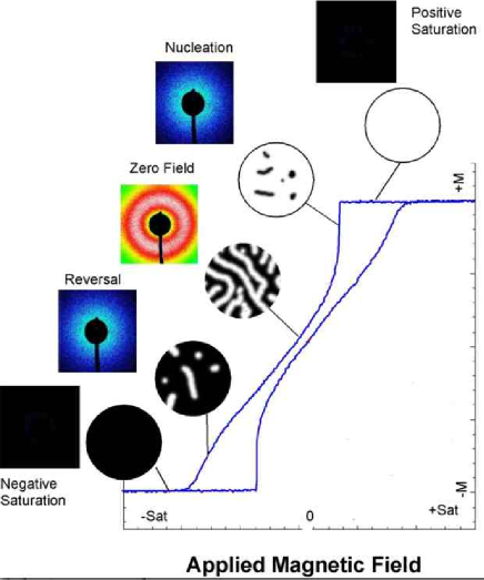
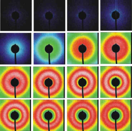
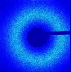
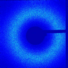
The typical evolution of the speckle patterns for one-half cycle around the major hysteresis loop for the 3 sample is schematically illustrated in Fig. 8. and the corresponding measured speckle patterns are shown in Fig. 9. Starting at positive saturation there is no magnetic contrast—all the magnetic domains are aligned with the field—consequently there is no magnetic scattering. As we descend from positive saturation the magnetic domains nucleate and produce a magnetic speckle pattern that is shaped like a cookie (disk). When we reach zero applied field, the magnetic domains have grown so much that they fill the entire sample; in this limit they must interact, and their interaction produces the donut (annular) shaped speckle pattern. When we reach the reversal region, the domain density is again low, and so the associated speckle pattern is again cookie shaped.

IV.1 Correlation Coefficients

To quantitatively compare the magnetic domain configurations versus the applied magnetic field history, we calculate the normalized correlation coefficients between pairs of our measured images acquired for different applied field histories. To date, our work has been primarily based on the normalized cross-correlation of these magnetic speckle patterns—our magnetic speckle fingerprints. However, this comparison can be done in reciprocal space—as we have primarily been doing up until now—or in real space as we are just beginning to do.

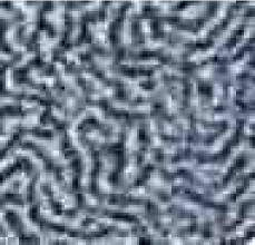
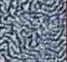
Some of our initial experimental work in real space is illustrated Figure 10 which shows the magnetic domains in our 8.5 mTorr sample measured using x-ray magnetic microscopy peter RSI . These images were recorded at the Co L3 edge using XM-1 at the ALS and were taken on the descending major loop; the left panel shows the domains at $H=-0.50$ kOe and the right panel shows the domains at $H=-1.00$ kOe. The correlation coefficients obtained from our real-space normalized cross-correlation analysis of the domain patterns agrees with our correlation coefficients obtained via our standard reciprocal-space normalized cross-correlation analysis of the corresponding speckle patterns. Therefore we believe that our real space and reciprocal space methods will prove to be complementary.

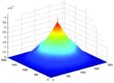
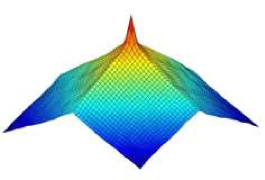
Our normalized cross-correlation analysis procedure in reciprocal space is illustrated in figures 11-13. Figure 11 shows the speckle fingerprints measured in reciprocal space; again the left panel shows the fingerprint at $H=-0.5$ and the right panel shows the fingerprint at $H=-1.0$ kOe. Figure 12 shows the calculated autocorrelation functions for these two speckle fingerprints. Note that both of these consist of a broad smooth “mountain” with a sharp “tree” on top of it.

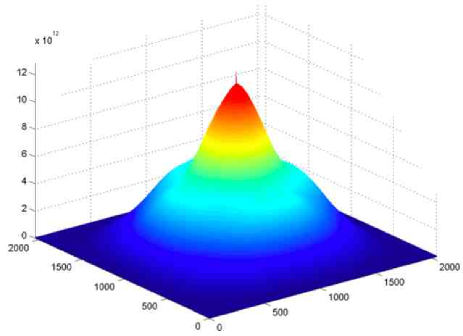
The mountain corresponds to the diffuse scattering envelope from the short range magnetic ordering and the tree corresponds to the coherent scattering from the entire illuminated area. Figure 13 shows the calculated cross-correlation function for the two speckle fingerprints shown in Fig. 12. Again there is an “diffuse mountain” with a “coherent tree” on top of it.

We want to use the coherent components of these auto- and cross-correlation functions to compute the normalized correlation coefficient. We extract the volume of each tree and then we calculate the ratio

\rho(a,b)=\frac{volume(a\otimes b)}{\big{[}{volume(a\otimes a)}\;\;{volume(b\otimes b)}\big{]}^{1/2}}.

The resulting normalized correlation coefficient $\rho(a,b)$ measures the normalized degree-of-correlation between any two speckle patterns. We use it to quantify the degree-of-correlation between pairs of speckle patterns which in turn is our measure of the degree-of-correlation between the corresponding magnetic domain patterns. When $\rho(a,b)=1$ the two magnetic domain patterns are identical, and when $\rho(a,b)=0$ the two magnetic domain patterns are completely different.

In general, the value of $\rho$ specifies the degree-of-correlation between the two speckle patterns which in turn are proportional to the Fourier coefficients of the magnetization density for the two magnetic domain configurations. Because our correlations are based on the intensity, we are unable to determine the sign of the correlations—we cannot distinguish correlation from anti-correlation. This is essentially Babinet’s Principle.

IV.2 Data Analysis

We now sketch the details of our correlation coefficient calculations. To determine the correlation between two speckle patterns, we generalized the standard correlation coefficient for two random variables $a$ and $b$ , which is given by

\rho(a,b)={\rm Cov}(a,b)\times\big{\{}{\rm Var}(a){\rm Var}(b)\big{\}}^{-1/2},

to the equivalent expression in terms of the background-subtracted cross-correlation function (ccf) and the background-subtracted autocorrelation functions (acf) of the speckle pattern intensities $I_{a}(q_{x},q_{y})$ and $I_{b}(q_{x},q_{y})$

\rho(a,b)=\frac{\sum{\rm ccf}(a,b)}{\big{[}{\sum\;{\rm acf}(a)\;\;\sum\;{\rm acf}(b)}\big{]}^{1/2}}

where the sums run only over the trees so that the background-subtracted auto- and cross-correlation functions contain only coherent scattering contributions.

We used the standard fast Fourier transform (FFT) to calculate the auto- and cross-correlation functions, but we first verified that the FFT produces precisely the same results as slow, sliding cross-correlation. Our speckle fingerprint images are 1024 by 1024 pixels, so they produce cross-correlation images with 2049 by 2049 points. The coherent speckle information, which is 2-3 pixels wide in the speckle patterns, is transformed into a peak 5-7 pixels wide in the correlation map. Figure 13 shows a typical cross-correlation map calculated using the two entire speckle patterns. Note that the shape of the mountain under the coherence tree is shaped like a rounded cone. When the tree gets small—as the two speckle patterns become almost uncorrelated—the rounded shape makes it tricky to subtract the background properly.

To provide information about the quality of our normalized cross-correlation values, we divided the whole speckle pattern into 8 to 15 square regions containing 100 by 100 pixels within which the intensity was nearly constant. In this way we removed the distortion produced by the shadow of the blocker, its support arm, and by camera defects and burns.

This piece-by-piece analysis made it much easier to separate the tree from the mountain. Because the variation in the average intensity over the small regions is much smaller than that over the entire image, the mountain now decays linearly away from the tree as shown in Fig. 14. Consequently, the small regions could always be reliably fit with simple linear functions. This made it much easier and more reliable to subtract the background.

It is also very useful to note that this type of speckle analysis completely separates the coherent signal from the diffuse, incoherent scattering present in an image. Indeed, so long as the speckle signal is identifiable and separable, then any incoherent signal is eliminated. This calculation is capable of introducing some error, however it is usually not sufficient to detract from the values obtained for the correlation coefficients. Even when the cross-correlation becomes difficult to identify, the correlation coefficient $\rho{\rm(a,b)}$ is still normalized by the auto-correlation of each image which remain well defined and comparably large.

V Experimental Results

As explained in the previous section, we used normalized correlation coefficients to extract information about the correlations between the magnetic domain configurations versus their applied-field history.

We addressed the following questions: Are the domains precisely the same each time we go around the major hysteresis loop? How are the domains related at the complementary points on the major loop? How are the domains related for different points within the same (ascending or descending) branch of the major loop? The first two questions are about major loop microscopic RPM and CPM, or inter-loop correlations. The third question is about major loop microscopic half-loop memory (HLM) values that probe the intra-branch correlations. We present our answers to these questions in turn below.

V.1 Major Loop Microscopic Return-Point Memory and Complementary-Point Memory

The first question that we addressed was whether our samples exhibited major loop microscopic RPM. To do so, we compared pairs of speckle patterns collected at the same point on the major loop, but separated by one or more full excursions around the major loop. The second question that we addressed was whether our samples exhibited major loop microscopic CPM. To do so, we compared pairs of speckle patterns collected at one point on the major loop with the speckle patterns collected at the inversion-symmetric complementary point on subsequent cycles.

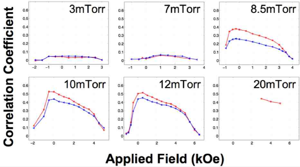
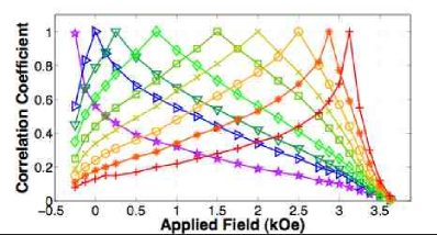
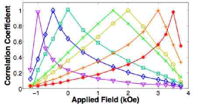
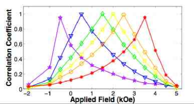
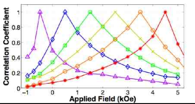
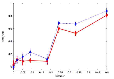
Our results for each sample are shown in Fig. 15, where the measured magnetic field dependence of the RPM and CPM correlation coefficients for each sample are shown. The data shown is for many excursions around each major loop. We did not observe any RPM or CPM for the 3 mTorr sample. The 7 mTorr sample exhibited an extremely small RPM and CPM—so small that we could not determine whether there was any RPM-CPM symmetry breaking. For all of our disordered samples, i.e., for 8.5 mTorr and above, we measured non-zero RPM and CPM values that had their RPM-CPM values slightly symmetry broken—our measured CPM coefficients are consistently a little smaller than the corresponding RPM coefficients. It is worth noting again that we verified with magnetometry that our samples demonstrated perfect macroscopic return point memory.

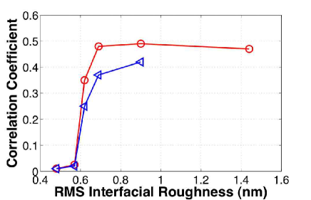
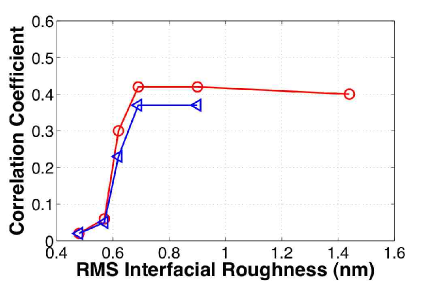
In order to properly compare the memory of the different samples, it is helpful to plot them using the same scale. By dividing each actual measured magnetization value, by the saturation magnetization for each sample we obtain a relative measure of the magnetization values. The value $M/M_{S}$ is known as the reduced magnetiztion $m$ . Fig. 16 shows our major loop microscopic RPM and CPM correlation coefficients, measured at room temperature for three values of the reduced magnetization, $m=-0.4$ , $m=0$ the coercive point, and $m=+0.4$ , for each sample. The RPM and CPM curves are plotted versus the sample’s measured rms roughness. As noted above, our smooth samples have essentially zero RPM and CPM values. In contrast, all of our rough samples exhibit RPM and CPM correlation coefficients that increase and saturate as the roughness increases, but never grow to unity. This increase starts precisely where the major loops change from being nucleation-dominated to being disorder-dominated.

In addition, our measurements establish the following interesting trends about the RPM and the CPM:

1.

Neither correlation coefficient depends on the number of intermediate loops between the correlated speckle patterns. This indicates that the deterministic components of the RPM and CPM are essentially stationary. This implies that the deterministic component of the memory in our system is largely reset by bringing the sample to saturation. It also strongly suggests that the same disorder is largely producing at least the deterministic component of both the RPM and the CPM.
2.

The RPM correlation coefficients are consistently a little larger than the CPM correlation coefficients. This demonstrates that the system acts in nearly the same way under positive and negative magnetic fields. So this implies that much of the disorder must have spin-reversal symmetry. This might be produced by random anisotropy, random bonds, or random coercivity, but not by random fields. This also suggests that the right physics might be captured by combining an RFIM model (which has RPM but essentially no CPM) with any of the other microscopic models (RAIM, RBIM, and RCIM) which all predict identical RPM and CPM.
3.

The correlation coefficients are largest near the initial domain reversal region. This suggests that the subsequent decorrelation is produced by the domain growth.
4.

The correlation coefficients decrease monotonically to their minimum values near complete reversal. This suggests that the decorrelation is produced by the domain reversal.

V.2 Half-Loop Memory (HLM); The Domain Configuration Correlations within a Single Branch of the Major Loop

We next studied the correlations between the magnetic domain configurations within a single half loop—i.e., the correlations within a single ascending, or a single descending, half loop. We looked for evidence that the evolution of the magnetic domains depended upon the disorder present in the sample. Does the level of the disorder influence how quickly or slowly the domain pattern evolves?

To study this question, we computed the normalized cross-correlation coefficient between the speckle patterns taken along a single ascending or descending half-loop. As we cycled each sample from negative to positive saturation, we stopped many times at fixed field values to record the speckle patterns. By cross correlating two speckle patterns collected on the same trip along the major hysteresis loop, we are able to determine how the domain configuration is changing.

Denoting the ordered set of descending speckle patterns by ${1,2,3,4,...}$ , we then calculated the correlation coefficients between all of the pairs of these speckle patterns:

•

$\rho(1,1),\rho(1,2),\rho(1,3),\rho(1,4),$ …. ,
•

$\rho(2,1),\rho(2,2),\rho(2,3),\rho(2,4),$ …. ,
•

$\rho(3,1),\rho(3,2),\rho(3,3),\rho(3,4),$ …. ,
•

etc.

This allowed us to correlate each of the domain configurations against all of the previous and subsequent measured configurations within the same descending branch of the major loop.

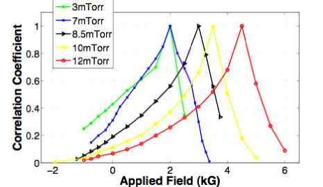
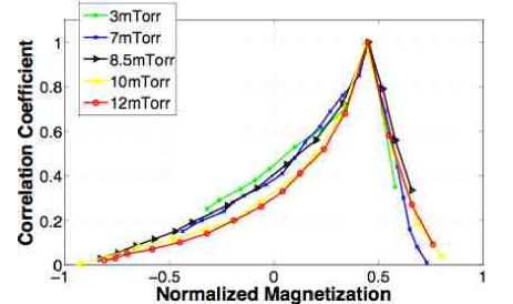
When the reference pattern was taken to be the image with its reduced magnetization $m=-0.4$ , the resulting half-loop memory (HLM) curves are shown versus the applied field in the top panel of Fig. 17; the bottom panel shows the same HLM curves plotted versus the reduced magnetization. Note the nice data collapse that occurs for the plots versus $m$ .

We found that the $m=-0.4$ HLM curves for our samples exhibit a subtle, but interesting dependance on their disorder. Although the HLM curves in the bottom panel of Fig. 17 look remarkably the similar, the low-disorder curves are systematically above the high-disorder curves. This indicates that the intra-loop domain configurations in the low-disorder samples are a little more persistent than those in the high-disorder samples. This is consistent with the idea that the domain widths in the low-disorder samples can expand and contract as the applied field is changed, whereas the domains in the high-disorder samples must break and reform.

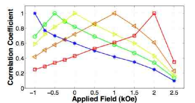
Fig. 18 shows the systematic evolution of our measured HLM curves versus each reference image for the 3, 7, 8.5, 10, and 12 mTorr samples. Up until now, there have been no analytic predictions or simulations for the shapes of, or the evolution of, these measured HLM curves.

VI Our New Theoretical Models

Our experimental results are the first direct measurements of the effects of controlled disorder on microscopic return-point memory and complementary-point memory. How can we understand our experimental results in the light of the current microscopic disorder theories, and, in particular, how does nature produce the RPM-CPM symmetry breaking? For spin models that are bilinear in spin (excluding the external field term), one might expect that the microscopic evolution of spins from a completely saturated state would lead to the same speckle patterns (or, with thermal noise or dynamical instabilities, to the same distribution of speckle patterns), whether one starts from a very large positive or very large negative applied field. As a consequence, the RPM and CPM correlation coefficients would be the same. Our experimental results show that this is not the case, and we have found that this apparent experimental small RPM-CPM symmetry breaking imposes strong constraints on any theory designed to describe the experiments.

In many theoretical descriptions of the magnetization process in systems with an easy anisotropy-axis, the local magnetization is described as a scalar quantity, since it is assumed that to a good approximation the magnetization must point along this easy axis. Starting from this point, we can obtain a number of different models according to the additional ingredients that we add. The well known Ising model is obtained by coupling neighboring spins ferromagnetically.

Many different microscopic disorder-induced memory systems have been constructed by introducing different types of disorder. The random anisotropy Ising model (RAIM) is produced by varying the local deviations from normal of the easy axisraim_vives . The random bond Ising model (RBIM) is produced by varying the strength of the ferromagnetic coupling between spinsrbim_vives . The random coercitivity Ising model (RCIM) is produced by varying the coercive field that is necessary to flip each spinrcim_friedman . The Edwards-Anderson spin-glass model (EASG) is produced by randomly choosing the signs of the bonds. An additional interesting and extensively studied possibility is to consider disorder entering in the form of a random local field acting on each spin. In this case, the model is called the random field Ising model (RFIM)sethna-dahmen . For compactness, below we will refer the above models using the acronym RXIM.

There is an important distinction among the previous models. The RAIM, RBIM, and RCIM are all spin inversion symmetric. So at zero temperature, they show perfect RPM and CPM. If temperature is included, then both the RPM and CPM become less than one, but they remain equal. The only model that is not spin symmetric, and can thereby explain the experimentally observed difference between RPM and CPM is the RFIM. The RFIM alone is too drastic because for all but extremely high disorder, it has essentially no CPM. This suggests one possible approach to explain our results: a theory that combines the RFIM with one of the other RXIMs possessing full CPM could produce a system which possesses slightly symmetry broken RPM and CPM. Another possible route to the broken RPM-CPM symmetry is via spin-glass models. The standard spin-glass model has perfect RPM and CPM at $T=0$ , but when coupled to random fields it exhibits imperfect CPM. Some of the relevant properties are summarized in Table 2.

We have explored the first two models, denoted Model 1 and Model 2 below, in the most detail. Specifically we tuned the model parameters to make the simulations behave as closely as possible to our experimental results. Both models were able to semi-quantitatively match our experimentally measured behavior for: (i) the domain configuration morphology, (ii) the shape of the major loops, (iii) the values of the RPM and CPM coefficients, and (iv) the small RPM-CPM symmetry breaking, versus both the disorder level and versus the magnetic-field-history.

We also explored one more model that was designed to produce the observed small RPM-CPM symmetry breaking with the minimum physics: Model 3 combines the RFIM with a spin-glass model. However, for this model, we have not yet tried to tune the model parameters to match the detailed experimental behavior. So we present it here as a minimal model that can produce a small RPM-CPM symmetry breaking that is qualitatively similar to that observed in our experiments.

Model 1 combines a pure RFIM with a pure RCIM jagla_1 ; jagla_2 . The essential idea was to produce a theory which combines the pure RFIM—with perfect zero-temperature RPM but essentially no CPM—with one of the other random Ising models possessing full CPM to thereby produce a model which possesses the experimentally observed slightly symmetry-broken RPM and CPM.

Model 2 explores the consequences of the type of dynamics used by the simulations to change the orientation of a spin ucsc_llg . All of the typical RXIM simulations use selection and update methods which are unchanged under a global spin flip. The next level of sophistication beyond simple scalar spin flips, is to use the vector Landau-Lifschitz-Gilbert (LLG) equation to describe the classical dynamics of the magnetic spins. However, this equation of motion is not spin symmetric. Consequently, the system will evolve differently than it does for simple spin flip dynamics. In fact, we found that the major loop for Model 2 does not exhibit perfect complementary symmetry.

Model 3 explores the consequences of mixing a RFIM with a spin-glass model helmut-gergely . Once again, because the RFIM has RPM but essentially no CPM, and the spin-glass model has both RPM and CPM, this model can be adjusted to exhibit a small RPM-CPM symmetry breaking.

The underlying symmetries and the predicted zero- and finite-temperature behavior of the RPM and CPM for the standard RXIMs and for the EASG model are shown in Table 2. The entries in this table shows the memories for the zero-temperature models. For the corresponding finite-temperature models, all of the “perfect” memories should be replaced by “imperfect”. The label “small” for the CPM represents the fact that at very high disorder the RFIM will show imperfect CPM. Our three models are presented and discussed one-by-one in more detail below.

Table 2: Symmetries and Memories of our Microscopic Disorder-Based Hysteresis Models

Disorder	RPM	CPM	Spin-inversion	Time-reversal
Model			symmetry	symmetry
RAIM	perfect	perfect	yes	yes
RBIM	perfect	perfect	yes	yes
RCIM	perfect	perfect	yes	yes
RFIM	perfect	small	no	yes
EASG	perfect	perfect	yes	yes

VI.1 Model 1: The RCIM plus the RFIM

The first model that we explored simulates localized magnetic moments that lie in a plane and point perpendicular to it. The local magnetization is taken to be a scalar variable $\phi$ . We include in Model 1 the long-range dipolar interactions, the short-range exchange interactions, and some sort of quenched disorder to simulate the effect of the interfacial roughness. In order to obtain more realistic results within a reasonable computational time, we used a continuous variable $\phi$ , instead of an Ising-like discrete variable. The numerical advantages provided by a continuous variable have previously been discussed in detail in jagla_1 .

The total Hamiltonian for Model 1 is

	$\displaystyle H=\alpha\int d{\bf r}\left(-\frac{\phi({\bf r})^{2}}{2}+\frac{\phi({\bf r})^{4}}{4}\right)-h\int d{\bf r}\phi({\bf r})$
	$\displaystyle+\beta\int d{\bf r}\frac{\left\|\nabla\phi({\bf r})\right\|^{2}}{2}+\gamma\int d{\bf r}d{\bf r}^{\prime}\phi({\bf r})\phi({\bf r}^{\prime})G({\bf r},{\bf r}^{\prime})$		(1)

For more details see jagla_1 .

The first term gives the local energy of the magnetic dipoles, favoring (but not forcing) the values $\phi=\pm 1$ . The second term includes the effect of an external magnetic field $h$ , and the third term provides the continuum version of a local ferromagnetic interaction. The dipolar interaction kernel $G$ is defined on a discrete numerical lattice by $G({\bf r},{\bf r}^{\prime})=1/|{\bf r}-{\bf r}^{\prime}|^{3}$ for ${\bf r}\neq{\bf r}^{\prime}$ , whereas $G({\bf r},{\bf r})\equiv 0$ . It has been shown that this particular regularization adopted at short distances does not play a crucial role in the results jagla_2 .

Disorder is included through the random spatial variation of $\alpha$ , namely $\alpha({\bf r})=\bar{\alpha}(1+\omega_{0}\eta({\bf r}))$ , where $\eta({\bf r})$ is a random spatial variable uniformly distributed between plus and minus one. Consequently, the constant $\omega_{0}$ controls the overall strength of the disorder. This way of introducing disorder corresponds to that in the RCIM. Other forms of introducing disorder in the system (particularly random anisotropy and random bond) should also be explored.

As anticipated above, Model 1 is spin symmetric, and consequently it will always predict RPM values equal to its CPM values. To explore the possibility that they could become different due to the existence of some symmetry breaking field we introduced disorder in the field through $h({\bf r})=\bar{h}(1+\omega_{1}\eta({\bf r}))$ . We always set $\omega_{1}<<\omega_{0}$ , so that the amount of disorder in the RFIM component was always much smaller than that in the RCIM component. The time evolution of the system is obtained through overdamped dynamics of the type

\frac{\partial\phi({\bf r})}{\partial t}=-\frac{\delta H}{\delta\phi({\bf r})}+\sqrt{2k_{B}T}\xi(t)

(2)

where for convenience, time has been rescaled and $\xi(t)$ is an uncorrelated white noise that simulates the effects of a temperature $T$ on the system.

Through a rescaling procedure, two of the coefficients in the Hamiltonian can be forced to take fixed values. In fact, we will assume that by appropriate time-, space-, and field-rescaling, the coefficients of the ferromagnetic and dipolar interactions (namely $\beta$ and $\gamma$ ) have been made equal to fixed values. For convenience in the simulations, these values were taken to be $\beta=2$ and $\gamma=0.19$ . The new parameters on which the model depends are now the rescaled values of $\alpha$ , $h$ , and $T$ . The results presented below correspond to simulations with $\alpha=1.8$ and $k_{B}T=2\times 10^{-4}$ for different values of the disorder set by $\omega_{0}$ and $\omega_{1}$ , and as a function of the external field $h$ .

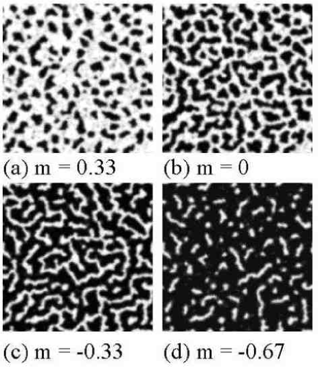
We tuned the model parameters to reproduce the experimental conditions. We started at magnetic saturation by applying a large external field $h$ , so that all the local moments point in the same direction. We then reduced the external field in small steps and obtained the “equilibrium configuration” by numerically solving the Hamiltonian equation until stationarity was obtained. Of course, the resulting “equilibrium configuration” is actually metastable. An example of the simulated magnetic domain configurations is shown in Fig. 19 for different applied fields.

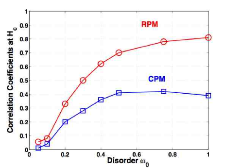
By using our scalar model with a ratio between the random field component and the random coercivity component of $\omega_{1}/\omega_{0}=0.04$ , we obtained the disorder-dependent correlation coefficients shown in Fig. 20. They were calculated using the domain configurations obtained from the simulation.

VI.1.1 The Effects of Combined Coercivity Disorder and Field Disorder on Memory

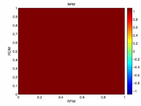
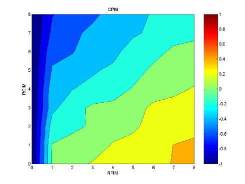
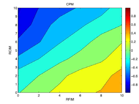
Now that we have demonstrated that a combined RCIM plus RFIM can be tuned to describe the resuts of our experiment quite well, it is natural to ask about the generic behavior of this combined model. In particular, how does its memory depend on its two disorders—the disorder in the coercivity and the disorder in the random field? We used a simple discrete-spin simulation to explore this question for both zero- and finite-temperature. Our simulations were performed on a 64 by 64 grid of dipolar-Ising spins. In dimensionless units, where the near-neighbor interaction energies are unity $J=1$ , our parameters were as follows: the random-field disorder was distributed normally with mean 0 and standard deviation $x/3$ ; the random-coercivity disorder was distributed normally with mean 0 and standard deviation $y$ . Note that $x$ and $y$ are the horizontal and vertical scales in Fig. 21.

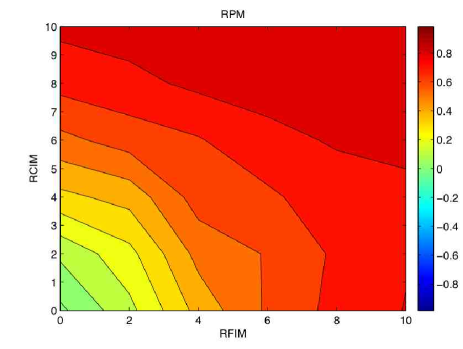
Our results for $T=0$ are shown in Fig. 21. Note that the RPM is perfect for both the RFIM and the RCIM, and that it is also perfect for any linear combination of the RFIM and RCIM. The CPM is perfect for the pure RCIM for all values of the random coercivity disorder, but the CPM is imperfect for the pure RFIM for all non-zero values of the random field disorder. The perfect CPM for both the pure Ising model and for the pure RCIM have perfect negative CPM values $\rho_{cpm}=-1$ . Consequently the magnetic domains at the complementary point are perfectly anti-correlated with the magnetic domains at the return point.

Our results for $T=0.1$ also are shown in Fig. 21. Note that the RPM for the pure Ising model is near zero, and that the RPM for the pure RFIM increases as the random field disorder is increased—it grows from zero with no random field disorder to about 1.0 at the highest disorders we explored. The RPM for the pure RCIM also increases as the random coercivity disorder is increased—it grows from zero with no random field disorder to 1.0 at the highest disorders we explored. The CPM for the pure Ising model is near zero. The CPM for the pure RFIM increases as the random field disorder is increased—it grows from zero with no random field disorder to about +0.4 at the highest disorders we explored. The CPM for the pure RCIM increases as the random coercivity disorder is increased—it grows from zero with no random field disorder to -1.0 at the highest disorders we explored. It is interesting to note that the magnitude of the correlations and anticorrelations is larger for the RCIM than the RFIM over the same range. The spin inversion symmetry of the RCIM pushes the system towards anti-correlation, favoring the same microscopic spin evolution on both sides of the major hysteresis loop. In contrast, because the RFIM does not possess spin-inversion symmetry, the random field can only drive the system towards positive correlation. Both of these compete to determine the sign and magnitude of the correlation coefficients. In the range where the contributions from the RCIM and RFIM are roughly equal, the CPM is uncorrelated while the RPM increases with the magnitude of each.

Although we have used a very simple discrete-spin simulation done on a 64 by 64 grid of dipolar-Ising spins, note that we obtain very similar behavior to that produced by our much more sophisticated and realistic model presented earlier.

VI.2 Model 2: The RAIM plus LLG Dynamics

There is another fundamental explanation for the observed RPM-CPM asymmetry ucsc_llg . Even when the Hamiltonian is constructed to possess spin-inversion symmetry, the dynamics describing how the magnetization changes do not have to be. In fact, the dynamics of the standard Landau-Lifschitz-Gilbert (LLG) equation break spin-inversion symmetry

\frac{d{\bf s}}{dt}=-{\bf s}\times({\bf B}-\gamma{\bf s}\times{\bf B}).

(3)

The first term describes the velocity with which a spin precesses about the magnetic field. The second term describes the damping of the precessional motion produced as the spin aligns along the magnetic field.

Under LLG dynamics, the spins undergo damped precessional motion about their local magnetic fields. When both the external field and all the spins are reversed, the orientation of each spin and its precesssion are reversed. The precessional motion of the spins (i.e., their motion perpendicular to their local fields) is not reversed, whereas the relaxational motion (parallel to the local fields) is reversed. As a consequence, for a disordered system, the evolution of the magnetic domains when starting from a large negative field is not the mirror image of the evolution starting from a large positive field.

Therefore the spin-inversion symmetry of the Hamiltonian that completely determines the equilibrium static properties does not control the non-equilibrium dynamics that are relevant for magnetic hysteresis. We first observed this effect for a vector spin model using the LLG equations to describe a set of magnetic nanopillars ucsc_llg . There we found that the major hysteresis loop was not symmetric under inversion of the applied field and the magnetization despite the fact that the Hamiltonian displayed this symmetry.

Model 2 that we describe below attempts to capture the physics of the magnetic domains in our experimental CoPt layered system and it has many parallels with the scalar approach described for Model 1 above. We will assume that (1) The films are disordered on the scales relevant to pattern formation, but are strongly anisotropic. (2) The easy axis has small random deviations away from the direction perpendicular to the film.

From electron micrographs of similar sputtered films, we see that the layers become increasingly rough and non-planar as the disorder is increased eric-prb . Consequently, even though the physics of the perfect material dictates a strong anisotropy, the local direction of the easy axis will no longer be precisely perpendicular to the film. Because it varies randomly in space, we write the anisotropic contribution to the Hamiltonian as

\mathcal{H}_{ani}=-\alpha\displaystyle\sum_{i}({\bf s}_{i}\cdot{\bf\hat{n}}_{i})^{2},

(4)

where $\alpha$ is a model parameter. Higher-order corrections that are even in $s_{i}$ are also possible, but they are not necessary to obtain qualitative agreement with our experiments.

Disorder is included through random variation in the easy axis $\hat{\mathbf{n}}_{i}$ for each block of spins. To adjust the effects of the disorder, a weighting factor $w_{ani}$ was included that controls the variation from the perpendicular axis. For small values of $w_{ani}$ the variation is small and there is little disorder. At larger values, the disorder is heavily weighted and has a large influence.

We have also included the short-range ferromagnetic coupling $J$ . Because we are attempting to model this system as a continuum, we take the usual approach of minimizing effects of the grid by writing this ferromagnetic interaction in terms of ${\bf s_{k}}$ , the Fourier transform of the spins

\mathcal{H}_{el}=J\displaystyle\sum_{\bf k}k^{2}s_{\bf k}^{2}.

(5)

As in the scalar case, it is also crucial to include the long-range dipolar interaction

\mathcal{H}_{dip}=-w_{dip}\displaystyle\sum_{i,j\neq i}\frac{3({\bf s}_{i}\cdot{\bf e}_{ij})({\bf e}_{ij}\cdot{\bf s}_{j})-{\bf s}_{i}\cdot{\bf s}_{j}}{r_{ij}^{3}},

(6)

where ${\bf r}_{ij}$ is the displacement vector between spins $i$ and $j$ , ${\bf e}_{ij}$ is the unit vector along this direction, and $w_{dip}$ represents the strength of the dipolar coupling.

Although this is correct for point dipoles, we are modeling blocks of spins and must include this effect in this interaction. In particular, the short-range behavior is smoothed out by integration in the vertical direction LangerGoldstein . We implement this as a k-space cutoff by multiplying the dipolar interaction in k-space by a Gaussian $\exp(-k^{2}d^{2}/2)$ where $d$ is a parameter comparable to the thickness of the sample.

Finally, we include the usual interaction with the external field

\mathcal{H}_{ext}=-B_{e}\displaystyle\sum_{i}s_{i}^{z}.

(7)

All of the terms in the Hamiltonian are bi-linear in the spins and the external field but, as discussed above, the LLG equations are not. Because of the symmetry breaking produced by the LLG dynamics, Model 2 can be tuned to produce a small RPM-CPM symmetry breaking similar to that measured by our experiments.

We have chosen the relaxation time to be of the order of the precessional period near saturating fields, that is $\gamma=1$ . Although this quantity has not been measured for our CoPt films, it has been measured for other similar materials. Experiments on NiFe films show that it is very large, approximately 100 Sandler , If it were so large in our CoPt system, it would only accentuate the memory asymmetry further. Work on CoCrPt systems Lyberatos has indicated that the precessional period is comparable to the relaxation time and if this is also true for our films, then our $\gamma=1$ assumption is reasonable.

Summarizing Model 2, we have coarse-grained vector spins evolving via the LLG equations with thermal noise. The Hamiltonian incorporates local ferromagnetic coupling, long-range dipolar forces, disordered anisotropy modeled by a random easy axis, and coupling to the external field. We found a range of model parameters that produced comparable behavior to that of our experimental samples.

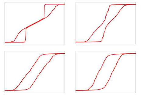
First, we examine the evolution of the major hysteresis loops versus the disorder. The evolution of the simulated major loops is shown in figure 22. The disorder increases from left to right and from top to bottom; the simulated loop shape for the lowest disorder is shown in the upper left panel and the simulated loop shape for the highest disorder is shown in the lower right panel.

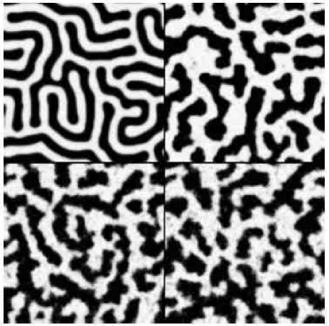
The simulated domain configurations for different amounts of disorder at a finite temperature are shown in Fig. 23. Again the disorder increases from left to right and from top to bottom. The evolution of our simulated domain configurations versus disorder qualitatively agrees with that observed in the experimental samples.

For low disorder when lowering the external field from saturation, our simulations show that there is suddenly spontaneous growth of domain lines that fill up the system at a critical value of the field; this happens at constant field. For our simulations with low disorder the domain morphology looks labyrinthine at remanence. The simulated morphology and growth of the domains is very similar to that of our experiments.

For low disorder, the simulated hysteresis loops look quite similar to those for the 3 mTorr samples: corresponding to the onset of domain growth in the simulation, there is a cliff in the hysteresis loop because the magnetization decreases substantially during this phase of growth. When the disorder is high, it pins the domains by destroying translational invariance. This happens suddenly in our simulations in a similar fashion as that in the experiments suggesting a “critical disorder” sethna-dahmen . For this “critical disorder” and above, the spontaneous cliff-producing growth of the domains disappears, and the domains at remanence no longer look labyrinthine, but instead are much more disordered. After losing their cliff-like shape, the simulated hysteresis loops are smooth. The qualitative similarities between the experimental major loops and the simulated major loops for Model 2 can be seen by a comparison of Fig. 22 and Fig. 6.

We explored the memory effects in Model 2 by calculating the correlation between pairs of domain configurations. Because we had direct access to the complete domain configurations, we calculated the correlations in real space. The simulated RPM and CPM values for Model 2 at the coercive point as a function of the disorder are shown in figure 24. The RPM-CPM symmetry breaking is clearly visible. As the temperature is increased, both curves lower in value but the RPM curve still remains slightly above the CPM curve. These curves clearly grow rapidly past the “critical disorder point” where the simulated and experimental loops change from cliff-like to smooth.

The observed memory behavior in Model 2 can be explained as follows. For low disorder, the spontaneous growth of the domains is very susceptible to thermal fluctuations. If we observe the growth of the domains for several cycles around the major loop, we find that although the initial nucleation points are precisely the same, the evolution past that point is different every time. For low disorder, it appears that the thermal fluctuations produce different domain patterns during each cycle. However, for high disorder, the pinning produced by the disorder appears to constrain the domain growth and leads to significant similarity from cycle to cycle of the domain configurations at the coercive point.

In summary, Model 2 simulated CoPt thin films using a spin symmetric Hamiltonian with LLG dynamics. Unlike in our other scalar models, the LLG vector dynamics is the mechanism for breaking the RPM and CPM symmetry. In addition to this asymmetry, Model 2 was also able to successfully simulate both the major hysteresis loops and the evolution of the domain configurations in qualitative agreement with our experimental results.

VI.3 Model 3: A Spin-Glass Model plus the RFIM

Motivated by the above experimental and theoretical results, we attempted to determine the minimal model that would capture the essential physics of the observed memory effects. In this section, we explore the following four questions: (1) What is the minimal model that exhibits these memory effects? (2) Do these memory effects persist at finite temperatures? (3) How do these memory effects depend on the disorder? and (4) Does the RPM-CPM symmetry breaking convincingly exceed the error bars? We assert that it is of general interest to study the RPM and CPM for simple paradigmatic models, such as the Edwards-Anderson Ising spin glass and the RFIM sethna-dahmen ; binder

VI.3.1 Ingredient 1: The Edwards-Anderson Spin-Glass

We start with the Hamiltonain for the Edwards-Anderson edwards spin glass (EASG) given by

{\mathcal{H}}_{\rm EASG}=-\sum_{\langle i,j\rangle}J_{ij}S_{i}S_{j}-H\sum_{i}S_{i}.

(8)

The spins $S_{i}=\pm 1$ lie on the vertices of a square lattice in two dimensions (2D) of size $N=L^{2}$ with periodic boundary conditions. The interactions $J_{ij}$ are Gaussian distributed with zero mean and standard deviation $\sigma_{J}$ . Our simulations were performed by first saturating the system by applying a large external field $H$ and then reducing $H$ in small steps to reverse the magnetization.

For finite temperatures, we performed a Monte Carlo simulation and equilibrated until the average magnetization was independent of time for each field step. For zero temperature, we used Glauber dynamics katzgraber where randomly chosen unstable spins—pointing against their local field $h_{i}=\sum_{\langle j\rangle}J_{ij}S_{j}+H$ —were flipped until all spins were stable for each field step. These simulations converged rapidly and showed essentially no size-dependence past $L=20$ .

We quantified the simulated RPM and CPM with $\rho_{r}(H)$ , the overlap in real space of the spin configuration at a field $H$ with the configuration at a field with the same magnitude $|H|$ after an $n=1/2$ cycle for CPM and $n=1$ cycle for RPM

\rho_{r}(H)=\frac{(-1)^{2n}}{N}\sum_{i=1}^{N}S_{i}(H)S_{i}^{(n)}(H)\;.

(9)

Our results for the EASG show that this system exhibits nearly complete RPM and CPM throughout the entire field range for $T=0$ . The strong CPM can be attributed to the spin-inversion symmetry of the system: upon reversing all spins $S_{i}$ and the magnetic field $H$ , the Hamiltonian transforms into itself. The observation of robust RPM and CPM answers question 1 by establishing the EASG as a minimal model displaying these memory effects. However, the simulated memory effects were not perfect even at $T=0$ . This was probably due to the stochastic nature of the updating: during each field sweep, the spins were selected randomly for updating. Therefore, even at $T=0$ , the spin configurations did not evolve entirely along the same valleys of the energy landscape. Our simulations at finite temperatures show that the RPM and CPM decreased with increasing temperature and remained finite, even though it would seem natural for the thermal fluctuations to completely wash out the microscopic memory rendering it macroscopic only.

By varying the disorder strength $\sigma_{J}$ in our EASG model we showed that the RPM and CPM increase dramatically with increasing disorder, in good agreement with the experiments. The physical reason behind this result lies in the fact that when the disorder is high the energy landscape develops a few preferable valleys and the system evolves along these optimal valleys. This is not the case for small disorder where several comparable shallow valleys without a single optimal path are present. Finally, in relation to question 4 it is noted that in the EASG the differences between the RPM and CPM are immeasurably small.

VI.3.2 Ingredient 2: The Pure Random-Field Ising Model

Next, we study the same memory effects in the 2D random-field Ising model (RFIM)

{\mathcal{H}}_{\rm RFIM}=-J\sum_{\langle i,j\rangle}S_{i}S_{j}-\sum_{i}[H+h_{i}]S_{i}\;,

(10)

here the random fields $h_{i}$ were chosen from a Gaussian distribution with zero mean and standard deviation $\sigma_{h}$ ( $J=1$ ). The main differences between the RFIM and the EASG are that the RFIM does not have frustration and does not have spin-inversion symmetry. We find that this RFIM model also shows memory effects which are again stable with respect to thermal fluctuations.

Regarding question 4, the RFIM deviates from the EASG results and correlates with the experiments: in the RFIM, the RPM and CPM are different. The RPM is larger than the CPM for all temperatures due to the lack of spin-inversion symmetry in the Hamiltonian. For intermediate-to-large values of the disorder, the CPM is negligible and, in the proximity of the coercive field, the CPM correlation is even negative. In contrast, the RPM is large in the RFIM. In particular, for $T=0$ the RPM is perfect due to the “no-crossing property” of the RFIM middleton . Consequently, the RPM-CPM symmetry breaking is large over much of the parameter space. Just as for the EASG, the RFIM memory increases due to the valleys in the energy landscape becoming more pronounced with increasing disorder.

VI.3.3 The Combined Spin-Glass Model plus the RFIM

Because of the way that our simulations for the pure EASG model and for the pure RFIM do not agree with the experiments, the following question immediately arises: Can a combined EASG and RFIM yield results comparable to the experiments—increasing memory with increasing disorder, together with the RPM-CPM symmetry breaking?

In order to test this, we introduced random fields into the EASG that act only on a small fraction (5%) of the spins in order to break the spin-inversion symmetry of the Hamiltonian [Eq. (8)]:

{\mathcal{H}}_{\rm SG+RF}=-\sum_{\langle i,j\rangle}J_{ij}S_{i}S_{j}-\sum_{i}[H+h_{i}]S_{i}\;.

(11)

The random bonds $J_{ij}$ were chosen from a Gaussian distribution with zero mean and standard deviation $\sigma_{J}$ . The random fields were chosen from a Gaussian distribution with zero mean and standard deviation unity.

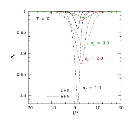
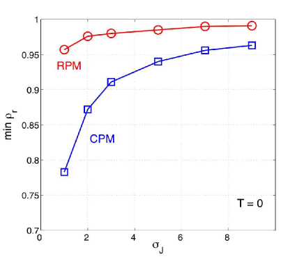
Since the dipolar interactions in our perpendicular anisotropy films are antiferromagnetic, they introduce extensive frustration into the system; this is the key ingredient for spin glasses. Our experimental system also contains several possible sources of random fields: spins frozen in by the local shape anisotropies produced by the locally deformed environments, unusually large crystal-field anisotropies, or by frozen-in reversed bubbles, as reported in the same experimental system by Davies et al. davies . Consequently, it is easy to imagine that all of the necessary ingredients for the combined EASG plus RFIM are likely to be present in our experimental samples. Results from Model 3 are shown in Fig. 25 and clearly resemble the experimental results presented earlier.

VI.3.4 Summary for Model 3

We now summarize our results for Model 3. We have found that our pure EASG model, our pure RFIM model, and our combined EASG model plus RFIM all exhibit both RPM and CPM, in which both memory effects persist to finite temperatures and both memory effects increase with increasing disorder. For our pure EASG model, the simulated RPM and CPM are identical because of the spin-inversion symmetry. For our pure RFIM, the RPM is always much larger than the CPM because of the lack of spin-inversion symmetry. Our combined ESAG and RFIM, a spin glass with diluted random fields that break the spin-inversion symmetry, reproduces the essential experimental results—it exhibits both RPM and CPM, both memory effects increase with increasing disorder, and the model can be tuned so that the RPM is a little bit larger than the CPM. All of these properties are present in Fig. 25. It will be exciting to see if experimentally realizable spin-glass systems can be shown to have these properties.

VII Conclusions

Our experimental results are the first direct measurements of the effects of controlled microscopic disorder on the magnetic memory of an ensemble of magnetic domains in the such perpendicular magnetic materials. We identified and studied three different aspects of the domain-level memory: microscopic return-point memory (RPM), microscopic complementary-point memory (CPM), and microscopic half-loop memory (HLM). Because our experimental observations could not be described by any existing microscopic-disorder-based theory, we developed new theories that do account for the behavior of our experimental system. Our combined experimental and theoretical work sets new benchmarks for future work.

We found a very rich behavior of these memory properties in our system of perpendicular-anisotropy multilayer CoPt samples. At the domain level, we found disorder-induced-partial RPM and CPM, and we also found a small RPM-CPM symmetry breaking where the RPM was consistently slightly larger than the CPM.

At the domain level, we found that the HLM versus the sample magnetization was very similar for all of our samples. There was only a subtle effect—the low disorder samples had slightly higher microscopic HLM than the high disorder samples. It was surprising to us that the HLM effects were nearly sample independent whereas the RPM and CPM effects were extremely sample dependent.

Our observed RPM and CPM are independent of the number of major loops separating the pairs of magnetic speckle fingerprints. This shows that the deterministic components of the RPM and CPM are essentially stationary, and implies that the deterministic memory in our system is largely reset by bringing the sample to saturation. It also strongly suggests that the same disorder is producing both the deterministic RPM and CPM.

Our measured RPM is consistently higher than our CPM. This slightly broken symmetry imposes severe limitations on the possible theoretical models. The evolution of the RPM and CPM with disorder is also very interesting. Both the RPM and CPM have their largest values just after the initial domain nucleation takes place and then diminish towards a minimum as saturation is approached. At room temperature, the memory is imperfect—the maximum measured RPM and CPM values are less than one. We suspect that this is due to the thermal fluctuations in our samples, but have not yet demonstrated this experimentally.

As we increase the disorder in our samples, there is initially little change in the memory, then at the same level of disorder there is a rapid increase in both the RPM and the CPM followed by apparent plateaus with the RPM slightly larger than the CPM. This is reminiscent of the disorder-induced transition predicted by the Sethna-Dahmen RFIM work where the major loop shape changes from a gradual loop to a sharp loop at a critical value of the disorder. At the corresponding “critical disorder transition” in our system, our loops also change shape, but more interestingly, and perhaps more importantly, both the RPM and CPM suddenly jump from zero to their maximum values.

Two possible explanations for RPM $>$ CPM in the disordered samples have been presented. Within the current experimental framework, it is not possible to determine which of these two methods is a more accurate description of our system.

There are potential physical mechanisms that would introduce random fields into our samples. Due to defects in the disordered samples, quenched spins may be present that do not reverse their direction even under the highest magnetic fields we were able to apply. In effect, even though the major loop hysteresis curve appears to be constant and unchanging, there may still be spins which persist in their original direction. These could be due to large crystal anisotropy, shape anisotropy because of the rough interfaces, or small, persistent magnetic bubbles due to incomplete saturation. In order to test for this scenario, it would be necessary to repeat the RPM and CPM measurements after saturating the samples under very high applied fields sufficient to saturate even the most stubborn spins.

In contrast, our dynamical model does not require the existence of these random fields. Instead it requires precessional motion to be present in the system. We know that spins precess in the presence of a magnetic field. However, we do not know the extent of precession relative to damping. Measurements of the ratio of the precessional and damping terms off the LLG equation on similar systems Sandler ; Lyberatos have shown that precessional motion is quite significant. More experiments will be necessary to determine if this is also the case for Co/Pt multilayer films. These two suggested experiments, study under very high applied fields and determination of the precessional to damping ratio, should shed light on the true mechanism for spin inversion symmetry breaking in this system.

There are very few direct, detailed studies of microscopic RPM, CPM, and HLM in either longitudinal or perpendicular magnetic materials and even fewer domain-level ensemble studies of such properties. It will be extremely interesting to see what our new coherent x-ray speckle metrology technique—together with our complementary x-ray magnetic microscopy studies—will teach us about the domain-level-ensemble memory in both of these technologically important and scientifically fascinating magnetic memory systems.

Acknowledgements.

We gratefully acknowledge the support of our work by the U.S. DOE via DE-FG02-04ER46102, DE-FG06-86ER45275, and DE-AC03-76SF00098, by the NSF via EAR-0216346, by the American Chemical Society via ACS-PRF 43637-AC10, and via the Alfred P. Sloan Foundation (K.L.).

References

(1) M. S. Pierce, R. G. Moore, L. B. Sorensen, S. D. Kevan, O. Hellwig, E. E. Fullerton, and J. B. Kortright, Phys. Rev. Lett. 90, 175502 (2003).
(2) “Random-Field Ising Models of Hysteresis,” J.P. Sethna, K.A. Dahmen, and O. Perkovic, cond-mat/0406320. Included in The Science of Hysteresis, Vol. II as Chapter 2. Ed. G. Bertotti and I. Mayergoyz, Academic Press, 2006.
(3) “The Barkhausen Effect,” G. Durin and S. Zapperi, cond-mat/0404512. Included in The Science of Hysteresis, Vol. II as Chapter 3. Ed. G. Bertotti and I. Mayergoyz, Academic Press, 2006.
(4) G. Durin and S. Zapperi, Phys. Rev. Lett. 84, 4075 (2000).
(5) Recently a number of groups have developed optical microscopy based Barkhausen apparatii. See, for example: S. Yang and J.L. Erskine, Phys. Rev. B 72, 064433 (2005); E. Puppin, Proceedings of the SPIE 5843, 23 (2004); D.H. Kim et al., ibid. p. 40; A. Schwartz and M. Liebmann, ibid. p. 52; K. Szielasko et al., Proceedings of the SPIE 5892, 105 (2004); O.M. Korpusov et al., J. Magn. Magn. Mater. 272-276, 2035 (2004); and references therein. However, because these marvelous new instruments use visible light, they cannot be used to study the sub-optically sized magnetic domains in our samples or in modern magnetic media.
(6) There has been some interesting work on memory properties, magnetic domains and reversal done in different systems by very different techniques. For a microscopy study, see: J. Ferré, V. Grolier, P. Meyer, S. Lemerle, A. Maziewski, E. Stefanowicz, S.V. Tarasenko, V.V. Tarasenko, M. Kisielewski, and D. Renard. Phys. Rev. B, 55, 15092, (1997). To see memory properties studied with magnetic waveforms see: J. R. Hoinville, R. S. Indeck, and M. W. Muller. IEEE Trans. Mag., 28, (1992).
(7) K. De’Bell, A.B. MacIsaac, J.P. Whitehead, Rev. Mod. Phys., 72, 1, 225, (2000).
(8) E.R. Madelung, Ann. d. Physik 17, 861 (1905). E.R. Madelung, Zeitschrift Physikalische 13, 486 (1912).
(9) F. Preisach, Z. Phys. 94, 277 (1935). For more recent work, see: I.D. Mayergoyz and G. Friedman, J. Appl. Phys. 61, 8, 4022, (1987); I.D. Mayergoyz, A.A. Adly, and G. Friedman, J. Appl. Phys. 67, 9, 5373, (1990).
(10) S.E. Zirka and Y.I. Moroz, IEEE Trans. on Magnetics, 31, 6, 3509,(1995); S.E. Zirka and Y.I. Moroz, IEEE Trans. on Magnetics, 35, 4, 2090, (1999); S.E. Zirka, Y.I. Moroz, and E. Della Torre, IEEE Trans. on Magnetics, 41, 9, 2426, (2005).
(11) M. S. Pierce, C. R. Buechler, L. B. Sorensen, J. J. Turner, S. D. Kevan, E. A. Jagla, J. M. Deutsch, T. Mai, O. Narayan, J. E. Davies, K. Liu, J. H. Dunn, K. M. Chesnel, J. B. Kortright, O. Hellwig, and E. E. Fullerton, Phys. Rev. Lett. 94, 017202 (2005).
(12) B. Hu, P. Geissbuhler, L. B. Sorensen, S. D. Kevan, E. E. Fullerton, and J. B. Kortright, Synch. Rad. News 14, 11 (2001).
(13) E. E. Fullerton, J. Pearson, C. H. Sowers, S. D. Bader, X. Z. Wu, and S. K. Sinha, Phys. Rev. B 48, 17432 (1993).
(14) O. Hellwig, G. Denbeau, J. B. Kortright and E. E. Fullerton, Physica B: Cond. Mat. 336, 136, (2003).
(15) J. E. Davies, O. Hellwig, E. E. Fullerton, G. Denbeaux, J. B. Kortright and Kai Liu, Phys. Rev. B, 70, 224434 (2004).
(16) C. Kooy and C. Enz, Philips Res. Reports 15, 7 (1960).
(17) J.W. Miao, Y. Nishino, Y. Kohmura, B. Johnson, C. Song, S.H. Risbud, and T. Ishikawa, Phys. Rev. Lett., 95, 085503, (2005); J.W. Miao, H. N. Chapman, J. Kirz, D. Sayre and K. O. Hodgson, Ann. Rev. Biophys. Biomol. Struct. 33, 157 (2004) and references therein.
(18) S. Eisebitt, J. Lüning, W. F. Schlotter, M. Lörgen, O. Hellwig, W. Eberhardt and J. Stöhr, Nature, 432, 885. (2004). O. Hellwig, S. Eisebitt, W. Eberhardt, J. Lüning, W. F. Schlotter and J. Stöhr J. Appl. Phys. 99, 08H307, (2006).
(19) C.C. Retsch and I. McNulty, Phys. Rev. Lett., 87, 077401, (2001).
(20) P. Fischer, T. Eimüller, G. Schütz, G. Denbeaux, A. Pearson, L. Johnson, D. Attwood, S. Tsunashima, M. Kumazawa, N. Takagi, M. Köhler and G. Bayreuther, Rev. Sci. Inst. 72, 2322 (2001).
(21) For the RAIM, see for example E. Vives and A. Planes, Phys. Rev. B, 63, 134431, (2001).
(22) For RBIM see E. Vives and A. Planes, J. Magn. Magn. Mater. 221, 164 (2000).
(23) For RCIM see O. Hovorka and G. Friedman, cond-mat/0306300 (2003).
(24) E. A. Jagla, Phys. Rev. E 70, 046204 (2004).
(25) E. A. Jagla, Phys. Rev. B 72, 094406 (2005).
(26) J.M.Deutsch, T. Mai, and O. Narayan, Phys. Rev. E, 71, 026120 (2005); J.M. Deutsch and T. Mai Phys. Rev. E, 72, 016115 (2005).
(27) H.G. Katzgraber and G.T. Zimányi, Phys. Rev. B 74, 020405(R) (2006)
(28) S. A. Langer, R. E. Goldstein and D. P. Jackson, Phys. Rev. A 46, 4894 (1992).
(29) G. M. Sandler, H. N. Bertram, T. J. Silva and T. M. Crawford, J. Appl. Phys. 85, 5080 (1999).
(30) A. Lyberatos, G. Ju, R. J. M. van de Veerdonk, and D. Weller, J. Appl. Phys. 91, 2236 2002.
(31) K. Binder, and A.P. Young, Rev. Mod. Phys. 58, 801 (1986); N. Kawashima and H. Rieger, cond-mat/0312432 (2003).
(32) S.F. Edwards, and P.W. Anderson, J. Phys. F: Met. Phys. 5, 965 (1975).
(33) H.G. Katzgraber, F. Pázmándi, C. R. Pike, K. Liu, R. T. Scalettar, K. L. Verosub, and G. T. Zimányi, Phys. Rev. Lett. 89, 257202 (2002).
(34) A.A. Middleton, Phys. Rev. Lett. 68, 670 (1992).