Microcanonical Approach to the Simulation of First-Order Phase Transitions.

Abstract

A generalization of the microcanonical ensemble suggests a simple strategy for the simulation of first order phase transitions. At variance with flat-histogram methods, there is no iterative parameters optimization, nor long waits for tunneling between the ordered and the disordered phases. We test the method in the standard benchmark: the $Q$-states Potts model ($Q\!=\!10$ in 2 dimensions and $Q\!=\!4$ in 3 dimensions), where we develop a cluster algorithm. We obtain accurate results for systems with $10^{6}$ spins, outperforming flat-histogram methods that handle up to $10^{4}$ spins.

Phase transitions are ubiquitous (formation of quark-gluon plasmas, evaporation/crystallization of ordinary liquids, Cosmic Inflation, etc.). Most of them are of (Ehrenfest) first order SANMIGUEL . Monte Carlo simulations MONTEBOOK are crucial for their investigation, but difficulties arise for large system linear size, $L$ (or space dimension, $D$). The intrinsic problem is that, at a first order phase transition, two (or more) phase coexist. The simulated system tunnels between pure phases by building an interface of size $L$. The free-energy cost of such a mixed configuration is $\Sigma L^{D-1}$ ($\Sigma$: surface tension), the interface is built with probability $\mathrm{exp}[-\Sigma L^{D-1}]$ and the natural time scale for the simulation grows with $L$ as $\mathrm{exp}[\Sigma L^{D-1}]$. This disaster is called exponential critical slowing down (ECSD).

No cure is known for ECSD in canonical simulations (cluster methods SWENDSEN-WANG ; WOLFF do not help), which motivated the invention of the multicanonical ensemble MULTICANONICAL . The multicanonical probability for the energy density is constant, at least in the energy gap $e^{\mathrm{o}}<e<e^{\mathrm{d}}$ ($e^{\mathrm{o}}$ and $e^{\mathrm{d}}$: energy densities of the coexisting low-temperature ordered phase and high-temperature disordered phase), hence the name flat-histogram methods MULTICANONICAL ; WANGLANDAU ; DEPABLO ; MASFLAT . The canonical probability minimum in the energy gap ($\propto\mathrm{exp}[-\Sigma L^{D-1}]$) is filled by means of an iterative parameter optimization.

In flat-histogram methods the system performs an energy random walk in the energy gap. The elementary step being of order $L^{-D}$ (a single spin-flip), one naively expects a tunneling time from $e^{\mathrm{o}}$ to $e^{\mathrm{d}}$ of order $L^{2D}$ spin-flips. But the (one-dimensional) energy random walk is not Markovian, and these methods suffer ECSD NEUSHAGER . In fact, for the standard benchmark (the $Q\!=\!10$ Potts model WU in $D\!=\!2$), the barrier of $10^{4}$ spins was reached in 1992 MULTICANONICAL , while the largest simulated system (to our knowledge) had $4\times 10^{4}$ spins WANGLANDAU .

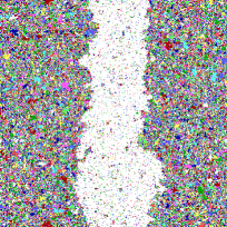
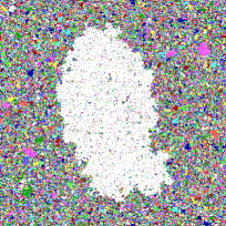
Figure 2: (Color online) $L=1024$ equilibrium configurations for the ferromagnetic $Q\!=\!10\,,D\!=\!2$ Potts model with periodic boundary conditions, at the 2 sides of the droplet-strip transition, namely $e=-0.809$ (left) and $e=-0.8$ (right).

ECSD in flat histogram simulations is probably understood NEUSHAGER : on its way from $e^{\mathrm{d}}$ to $e^{\mathrm{o}}$, the system undergoes several (four in $D\!=\!2$) “transitions”. First comes the condensation transition CONDENSATION ; NEUSHAGER , at a distance of order $L^{-D/(D+1)}$ from $e^{\mathrm{d}}$, where a macroscopic droplet of the ordered phase is nucleated. Decreasing $e$, the droplet grows to the point that, for periodic boundary conditions, it reduces its surface energy by becoming a strip DROPLETSTRIP , see Fig. 2 (in $D\!=\!3$, the droplet becomes a cylinder, then a slab LUIS2 ). At lower $e$ the strip becomes a droplet of disordered phase. Finally, at the condensation transition close to $e^{\mathrm{o}}\,,$ we encounter the homogeneous ordered phase.

Here we present a method to simulate first order transitions without iterative parameter optimization nor energy random walk. We extend the configuration space as in Hybrid Monte Carlo HYBRID : to our $N$ variables, $\sigma_{i}$ (named spins here, but they could be atomic positions) we add $N$ real momenta, $p_{i}$. The microcanonical ensemble for the $\{\sigma_{i},p_{i}\}$ offers two advantages. First, microcanonical simulations LUSTIG are feasible at any value of $e$ within the gap. Second, we obtain Fluctuation-Dissipation Eqs. (5–8) where the (inverse) temperature $\hat{\beta}$, a function of $e$ and the spins, plays a role dual to that of $e$ in the canonical ensemble. The $e$ dependence of the mean value $\langle\hat{\beta}\rangle_{e}$, interpolated from a grid as it is almost constant over the gap, characterizes the transition. We test the method in the $Q$-states Potts model, for which we develop a cluster algorithm. We handle systems with $10^{6}$ spins for $Q\!=\!10$ in $D\!=\!2$ and for $Q\!=\!4$ in $D\!=\!3$ (where multibondic simulations handle $N=10^{4}$ JANKE-PRIV ).

Let $U$ be the spin Hamiltonian. Our total energy is

$${\cal E}=\sum_{i=1}^{N}\frac{p_{i}^{2}}{2}\ +\ U\,,\quad(e\equiv{\cal E}/N\,,\ u\equiv U/N)\,.$$ (1)

In the canonical ensemble , the $\{p_{i}\}$ are a trivial gaussian bath decoupled from the spins. Note that, at inverse temperature $\beta$, one has $\langle e\rangle_{\beta}=\langle u\rangle_{\beta}+1/(2\beta)\,$.

Microcanonically, the entropy density, $s(e,N)$, is given by ($\sum_{\{\sigma_{i}\}}$: summation over spin configurations)

$$\mathrm{exp}[Ns(e,N)]=\int_{-\infty}^{\infty}\prod_{i=1}^{N}\mathrm{d}p_{i}\sum_{\{\sigma_{i}\}}\ \delta(Ne-\cal{E})\,,$$ (2)

or, integrating out the $\{p_{i}\}$ using Dirac’s delta function,

$$\mathrm{exp}[Ns(e,N)]=\frac{(2\pi N)^{N/2}}{N\Gamma(N/2)}\,\sum_{\{\sigma_{i}\}}\,(e-u)^{\frac{N}{2}-1}\theta(e-u)\,.$$ (3)

The Heaviside step function, $\theta(e-u)$, enforces $e>u$. The microcanonical average at fixed $e$ of a generic function of $e$ and the spins, $O(e,\{\sigma_{i}\})$, is (see Eq. (3) and LUSTIG )

$$\langle O\rangle_{e}\equiv\frac{\sum_{\{\sigma_{i}\}}\,O(e,\{\sigma_{i}\})\,(e-u)^{\frac{N}{2}-1}\theta(e-u)}{\sum_{\{\sigma_{i}\}}(e-u)^{\frac{N}{2}-1}\theta(e-u)}\,.$$ (4)

The Metropolis simulation of Eq. (4), is straightforward.

Calculating $\mathrm{d}s/\mathrm{d}e$ from Eq.(3) we learn that  

$$\frac{\mathrm{d}s(e,N)}{\mathrm{d}e} = \langle\hat{\beta}(e;\{\sigma_{i}\})\rangle_{e}\,,$$ (5)

$$\hat{\beta}(e;\{\sigma_{i}\}) = \frac{N-2}{2N(e-u)}\,.$$ (6)

Fluctuation-Dissipation follows by derivating Eq. (4):

$$\frac{\mathrm{d}\langle O\rangle_{e}}{\mathrm{d}e}=\left\langle\frac{\partial O}{\partial e}\right\rangle_{e}+N\left[\langle O\hat{\beta}\rangle_{e}-\langle O\rangle_{e}\langle\hat{\beta}\rangle_{e}\right]\,.$$ (7)

As in the canonical case REWEIGHT , an integral version of (7) allows to extrapolate $\langle O\rangle_{e^{\prime}}$ from simulations at $e\geq e^{\prime}$:

$$\langle O\rangle_{e^{\prime}}=\frac{\left\langle O(e^{\prime};\{\sigma_{i}\})\,\theta(e^{\prime}-u)\left[\frac{e^{\prime}-u}{e-u}\right]^{\frac{N}{2}-1}\right\rangle_{e}}{\left\langle\,\theta(e^{\prime}-u)\left[\frac{e^{\prime}-u}{e-u}\right]^{\frac{N}{2}-1}\right\rangle_{e}}\,.$$ (8)

For $e<e^{\prime}$, configurations with $e<u<e^{\prime}$, suppressed by a factor $(e^{\prime}-u)^{N/2-1}$, are ignored in (8). Since we are limited in practice to $|e-e^{\prime}|\leq\sqrt{\langle u^{2}\rangle_{e}-\langle u\rangle_{e}^{2}}/|\mathrm{d}\langle u\rangle_{e}/\mathrm{d}e|\sim N^{-1/2}$, the restriction $e\geq e^{\prime}$ can be dropped, as it is numerically negligible.

The canonical probability density for $e$, $P_{\beta}^{(L)}(e)\propto\mathrm{exp}[N(s(e,N)-\beta e)]$ follows from $\langle\hat{\beta}\rangle_{e}$:

$$\log P_{\beta}^{(L)}(e_{2})-\log P_{\beta}^{(L)}(e_{1})=N\int_{e_{1}}^{e_{2}}\mathrm{d}e\,\left(\langle\hat{\beta}\rangle_{e}-\beta\right)\,.$$ (9)

In the thermodynamically stable region (i.e. $\mathrm{d}\langle\hat{\beta}\rangle_{e}/\mathrm{d}e<0$), there is a single root of $\langle\hat{\beta}\rangle_{e}=\beta$, at the maximum of $P_{\beta}^{(L)}$. But, see Fig. 1, in the energy gap $\langle\hat{\beta}\rangle_{e}$ has a maximum and a minimum ($L$-dependent spinodals SANMIGUEL ), and there are several roots of $\langle\hat{\beta}\rangle_{e}=\beta$. The rightmost (leftmost) root is $e_{L}^{\mathrm{d}}(\beta)$ ($e_{L}^{\mathrm{o}}(\beta)$), a local maximum of $P_{\beta}^{(L)}$ corresponding to the disordered (ordered) phase. We define $e_{L}^{*}(\beta)$ as the second rightmost root of $\langle\hat{\beta}\rangle_{e}=\beta$.

At the finite-system (inverse) critical temperature, $\beta_{\mathrm{c}}^{L}$, one has HEIGHT $P_{\beta_{\mathrm{c}}^{L}}^{(L)}(e_{L}^{\mathrm{d}}(\beta_{\mathrm{c}}^{L}))=P_{\beta_{\mathrm{c}}^{L}}^{(L)}(e_{L}^{\mathrm{o}}(\beta_{\mathrm{c}}^{L}))$, which is equivalent, Eq. (9) and JANKEMIC , to Maxwell’s construction:

$$0=\int_{e^{\mathrm{o}}_{L}(\beta_{\mathrm{c}}^{L})}^{e^{d}_{L}(\beta_{\mathrm{c}}^{L})}\mathrm{d}e\,\left(\langle\hat{\beta}\rangle_{e}-\beta_{\mathrm{c}}^{L}\right)\,,$$ (10)

(for large $N$, $\beta_{\mathrm{c}}^{\infty}-\beta_{\mathrm{c}}^{L}\propto 1/N\,$ BORGS-KOTECKY ). Actually, at fixed $e$ in the gap, also $\langle\hat{\beta}\rangle_{e}$ tends to $\beta_{c}^{\infty}$ for large $N$. In the strip phase it converges faster than $\beta_{\mathrm{c}}^{L}$, see Table 1.

In a cubic box the surface tension is estimated as 

$$\Sigma^{L}=\frac{N}{2L^{D-1}}\int_{e^{*}_{L}(\beta_{\mathrm{c}}^{L})}^{e^{\mathrm{d}}_{L}(\beta_{\mathrm{c}}^{L})}\mathrm{d}e\,\left(\langle\hat{\beta}\rangle_{e}-\beta_{\mathrm{c}}^{L}\right)\,.$$ (11)

$L\to\infty$ extrapolations $\Sigma^{\infty}-\Sigma^{L}\propto 1/L$ BINDER are popular.

As for the specific heat, for $N\to\infty$ the inverse function of the canonical $\langle e\rangle_{\beta}$ is the microcanonical $\langle\hat{\beta}\rangle_{e}$:

$$\frac{\mathrm{d}\langle u\rangle_{\beta}}{\mathrm{d}\beta}\approx\left[\frac{1}{2\langle\hat{\beta}\rangle_{e}^{2}}+\frac{1}{\mathrm{d}\langle\hat{\beta}\rangle_{e}/\mathrm{d}e}\right]_{e=\langle e\rangle_{\beta}}\equiv C_{L}(e)\,.$$ (12)

For large $N$, $e^{\mathrm{d}}_{L}(\beta_{\mathrm{c}}^{L})\,$, $e^{\mathrm{o}}_{L}(\beta_{\mathrm{c}}^{L})\,$, $C_{L}(e^{\mathrm{d}}_{L}(\beta_{\mathrm{c}}^{L}))\,$, $C_{L}(e^{\mathrm{d}}_{L}(\beta_{\mathrm{c}}^{L}))\,$ tend to $e^{\mathrm{d}}$, $e^{\mathrm{o}}$, or the specific heat of the coexisting phases (we lack analytical hints about convergence rates).

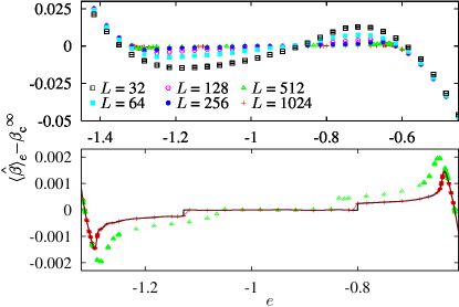
Figure 1: (Color online) Excess of $\langle\hat{\beta}\rangle_{e}$ over $\beta_{\mathrm{c}}^{L=\infty}$ vs. $e$, for the $Q\!=\!10$, $D\!=\!2$ Potts model and several system sizes. Bottom: magnification for $L\geq 512$. The flat central region is the strip phase (the strip width varies at fixed surface free-energy). Lines (shown for $L=1024$) are the two interpolations used for $L\geq 512$. We connect 3 independent cubic splines, in the strip phase and in its sides, either by a linear function or by a step-like $1/100$ power. Differences among the two interpolations are used to estimate the error induced by the uncertainty in the location of the strip-droplet transitions.

We now specialize to the Potts model WU . The spins $\sigma_{i}=0,1,\ldots,Q-1\,,$ live in the $N=L^{D}$ nodes of a (hyper)cubic lattice of side $L$ with periodic boundary conditions, and interaction ($<ij>$: lattice nearest-neighbors)

$$U=-\sum_{<ij>}\delta_{\sigma_{i},\sigma_{j}}\,.$$ (13)

A cluster method is feasible. Let $\kappa$ be a tunable parameter and $w(e,u,\kappa)=(e-u)^{N/2-1}\,\mathrm{exp}[\kappa Nu]\theta(e-u)$. Our weight is $w(e,u,\kappa)\mathrm{exp}[-\kappa U]\,,$ see (4), or, introducing bond occupation variables, $n_{ij}=0,1$, and $p\equiv 1-\mathrm{exp}[\kappa]$,

$$w(e,u,\kappa)\prod_{<i,j>}\left[(1-p)\delta_{n_{ij},0}\ +\ p\,\delta_{n_{ij},1}\delta_{\sigma_{i},\sigma_{j}}\right]\,,$$ (14)

which is the canonical statistical weight at $\beta\!=\!\kappa$ EDWARDS-SOKAL , but for the $\{n_{ij}\}$ independent factor $w(e,u,\kappa)$. Hence, clusters are traced in the standard way, but we accept a single-cluster flip WOLFF with Metropolis probability $p(e,\kappa)=\mathrm{min}\{1,w(e,u^{\mathrm{final}},\kappa)/w(e,u^{\mathrm{initial}},\kappa)\}\,$. Eqs.(5–8) suggest that $\kappa=\langle\hat{\beta}\rangle_{e}$ maximizes $p(e,\kappa)\,$ (a short Metropolis run provides a first $\kappa$ estimate). We obtain $\langle p(e,\kappa)\rangle_{e}>0.99$ for $e\leq e^{\mathrm{d}}$, and still $\langle p(e,\kappa)\rangle_{e=e^{\mathrm{o}}}>0.78$.

We simulated the ($Q\!=\!10$,$D\!=\!2$) Potts model BAXTER , for $L=32,64,128,256,512$ and $1024$, sampling $\langle\hat{\beta}\rangle_{e}$ at 30 points evenly distributed in $-1.41666\leq e\leq-0.45\,.$ For $L=512$, we made 15 extra simulations to resolve the narrow spinodal peaks (26 extra points for $L=1024$). Our Elementary Monte Carlo Step (EMCS) was: $\mathrm{max}\{10,N/(\langle{\cal N}\rangle_{e}\langle p(e,\kappa)\rangle_{e})\}$ cluster-flip attempts (${\cal N}$: number of spins in the traced cluster; it is of order one at $e^{\mathrm{d}}$ and of order $N$ at $e^{\mathrm{o}}$). So, every EMCS we flip at least $N$ spins. For each $e$, we performed $2\times 10^{6}$ EMCS, dropping the first $10\%$ for thermalization. A similar computation was carried out for the ($Q\!=\!4$,$D\!=\!3$) Potts model JANKEQ4 (for details see Table 1 and INPREPARATION ).

Our $\langle\hat{\beta}\rangle_{e}$ in $D\!=\!2$ is shown in Fig. 1. Data reweigthing (8) was used only to reconstruct the narrow spinodal peaks. To find the roots of $\langle\hat{\beta}\rangle_{e}=\beta$, or to calculate the integrals in Eqs. (10,11), we interpolated $\langle\hat{\beta}\rangle_{e}$ using a cubic spline . For $L\geq 512$ the strip-droplet transitions produce two “jumps” in $\langle\hat{\beta}\rangle_{e}$, causing oscillations in the interpolation (Gibbs phenomenon), cured by either of two interpolation schemes, see Fig. 1.

We obtain $\beta_{\mathrm{c}}^{L}\,$, $\Sigma^{L}\,$, $e^{\mathrm{o}}_{L}(\beta_{\mathrm{c}}^{L})\,$, $e^{\mathrm{d}}_{L}(\beta_{\mathrm{c}}^{L})\,$, $C_{L}(e^{\mathrm{o}}_{L}(\beta_{\mathrm{c}}^{L}))\,$ and $C_{L}(e^{\mathrm{d}}_{L}(\beta_{\mathrm{c}}^{L}))\,$ from the interpolation of $\langle\hat{\beta}\rangle_{e}$, and of $\mathrm{d}\langle\hat{\beta}\rangle_{e}/\mathrm{d}e$, see (7). Statistical errors are Jack-Knife’s  VICTORAMIT (the $i$-th block is obtained interpolating the $i$-th Jack-Knife blocks for $\langle\hat{\beta}\rangle_{e}$). There are also interpolation and integration errors. Fortunately, errors of order $\epsilon$ in $e^{\mathrm{o}}_{L}(\beta_{\mathrm{c}}^{L})$ or $e^{\mathrm{d}}_{L}(\beta_{\mathrm{c}}^{L})$ yield errors of order $\epsilon^{2}$ in $\beta_{\mathrm{c}}^{L}$: the main error in $\beta_{\mathrm{c}}^{L}$ is the quadrature error for $\langle\hat{\beta}\rangle_{e}$ divided by the latent heat. On the other hand, $e^{*}_{L}(\beta_{\mathrm{c}}^{L})$ is near to the droplet-strip transition, and an error on it does have an impact on $\Sigma_{L}$.

In Table 1 are our results for ($D\!=\!2,Q\!=\!10$) and the known large $L$ limits. A fit for $c$ in $\beta_{\mathrm{c}}^{\infty}-\beta_{\mathrm{c}}^{L}=c/L^{D}$ BORGS-KOTECKY is unacceptable for $L\geq 32$ ($\chi^{D}/\mathrm{d.o.f.}=14.32/4$), but good for $L\geq 64$ ($\chi^{D}/\mathrm{d.o.f.}=1.77/3$): our accuracy allows to detect subleading corrections. A fit $e^{\mathrm{o}}_{L}(\beta_{\mathrm{c}}^{L})-e^{\mathrm{o}}=b_{1}/L^{D}$ works only for $L\geq 256$ ($\chi^{2}/\mathrm{d.o.f.}=1.90/2$; for $e^{\mathrm{d}}_{L}(\beta_{\mathrm{c}}^{L})$ we get $\chi^{2}/\mathrm{d.o.f.}=1.41/2$). However, $\beta^{\mathrm{strip},L}$ (see caption to Table 1) is compatible with $\beta_{\mathrm{c}}^{\infty}$ for $L\geq 256$. Then, the simplest strategy to get $\beta_{\mathrm{c}}^{\infty}$ and the latent heat is: (1) for $L$ large enough to display a strip phase, locate it with short runs, (2) get $\beta^{\mathrm{strip},L}$ accurately, and (3) find the leftmost(rightmost) root for $\langle\hat{\beta}\rangle_{e}=\beta^{\mathrm{strip},L}$.

As for $\Sigma^{L}$, the inequality $\Sigma^{\infty}\leq 0.0473505$ JANKESIGMA (equality under the hypothesis of complete wetting) was violated by $1/L$ extrapolations performed with $L\leq 100$ MULTICANONICAL . The reader may check (Table 1) that our data for $L\leq 256$ extrapolate above 0.0473505, but drop below for $L\geq 512$. Indeed, the consistency of our results for $\beta_{\mathrm{c}}^{L}$ imply that the integration error for $\langle\hat{\beta}\rangle_{e}$ is (at most) $2\times 10^{-6}$ for $L=1024$. Hence, the integration error for $\Sigma_{L}$ is at most $10^{-3}$. Adding it to the difference between the linear and the step-like interpolation, Fig. 1, we obtain $\Sigma^{L=1024}=0.043(2)$, which is slightly below 0.0473505.

As for ($Q\!=\!4$, $D\!=\!3$), see Table 1, $\beta^{\mathrm{strip},L}$ has converged (within accuracy) for $L\geq 64$. Hence, our preferred estimate is $\beta_{\mathrm{c}}^{\infty}\!=\!0.6286206(10)$, that may be compared with Janke and Kapler’s $\beta_{\mathrm{c}}^{\infty}\!=\!0.62863(2)$ JANKEQ4 . Accordingly, we find $e^{\mathrm{o}}(\beta^{\mathrm{strip},L})\!=\!-1.10537(4)$, $e^{\mathrm{d}}(\beta^{\mathrm{strip},L})\!=\!-0.52291(2)$, $C_{L}(e^{\mathrm{o}}(\beta^{\mathrm{strip},L}))\!=\!35.4(9)$, and $C_{L}(e^{\mathrm{d}}(\beta^{\mathrm{strip},L}))\!=\!4.24(18)$. The reader will note that $\beta_{\mathrm{c}}^{L\!=\!128}$ is far too high (for instance, from the $\chi^{2}/\mathrm{d.o.f.}$ of the extrapolation $\beta_{\mathrm{c}}^{L}\!=\!\beta_{\mathrm{c}}^{\infty}+cL^{-D}$). Therefore, the integration error is $\sim 4\times 10^{-6}$ (larger than the statistical one), which provides a bound for the error in the surface tension: $\Sigma^{L=128}\!=\!0.0118(4)$. This is compatible with $\Sigma^{L=64}$, and provides a reasonable $\Sigma^{\infty}$.

$L^{D}$	$\beta_{\mathrm{c}}^{L}$	$\Sigma^{L}$	$-e^{\mathrm{o}}_{L}(\beta_{\mathrm{c}}^{L})$	$-e^{\mathrm{d}}_{L}(\beta_{\mathrm{c}}^{L})$	$-C_{L}(e^{\mathrm{o}}_{L}(\beta_{\mathrm{c}}^{L})$	$-C_{L}(e^{\mathrm{d}}_{L}(\beta_{\mathrm{c}}^{L}))$	$\beta^{\mathrm{strip},L}$
$32^{2}$	1.423082(17)	0.05174(9)	1.3318(2)	0.5736(3),	5.13(13)	3.99(7)	1.42028(7)
$64^{2}$	1.425287(9)	0.05024(11)	1.3220(2)	0.5999(2)	6.44(17)	5.78(19)	1.42479(4)
$128^{2}$	1.425859(7)	0.049225(14)	1.31676(16)	0.61164(16)	7.4(3)	7.8(3)	1.42592(2)
$256^{2}$	1.426021(5)	0.0488(2)	1.31478(8)	0.61578(8)	8.0(3)	8.7(4)	1.42606(2)
$512^{2(A)}$	1.426051(4)	0.0473(3)	1.31392(6)	0.61710(4)	8.6(4)	9.1(4)	1.426048(12)
$512^{2(B)}$	1.426048(4)	0.0467(4)	1.31390(6)	0.61708(5)	8.6(4)	9.1(4)	1.426048(12)
$1024^{2(A)}$	1.4260599(19)	0.0430(3)	1.31375(3)	0.61748(3)	9.7(5)	8.7(4)	1.426066(9)
$1024^{2(B)}$	1.4260600(18)	0.0424(2)	1.31375(3)	0.61748(3)	9.7(5)	8.7(4)	1.426066(9)
$\infty^{2}$	1.4260624389…	$\Sigma^{\infty}\leq 0.0473505$	1.3136366978…	0.6175872662…	—	—	1.4260624389…
$8^{3}$	0.627394(7)	0.005591(10)	1.1553(7)	0.51412(12)	23.0(5)	3.856(16)	0.62625(4)
$16^{3}$	0.628440(3)	0.007596(6)	1.1189(4)	0.51818(5)	30.1(8)	3.620(13)	0.626687(15)
$32^{3}$	0.6285957(10)	0.009824(6)	1.10751(15)	0.522066(16)	34.2(9)	4.019(17)	0.627889(6)
$64^{3}$	0.6286133(7)	0.011557(6)	1.10542(8)	0.522831(8)	33.2(9)	4.11(2)	0.628621(3)
$128^{3(A)}$	0.6286237(5)	0.011778(7)	1.10548(3)	0.52293(2)	35.4(9)	4.25(17)	0.6286206(10)
$128^{3(B)}$	0.6286239(5)	0.011674(9)	1.10549(2)	0.52293(2)	35.4(9)	4.25(17)	0.6286206(10)

Table 1: System size dependent estimates of the quantities characterizing the first order transition, as obtained for the $Q\!=\!10,D\!=\!2$ Potts model (top) and $Q\!=\!4,D\!=\!3$ (bottom). Errors are Jack-Knife’s. Also shown is $\beta^{\mathrm{strip,L}}\!=\!\langle\hat{\beta}\rangle_{e=-0.95}$ (for $D\!=\!2$) or $\beta^{\mathrm{strip,L}}\!=\!\langle\hat{\beta}\rangle_{e=-0.764443}$ (for $D\!=\!3$), in the strip phase. The $\infty^{2}$ row contains exact results BAXTER and an inequality JANKESIGMA , for $D\!=\!2$, $Q\!=\!10\,$. The results with superscript $A$($B$) were obtained with the linear(step-like) interpolation scheme, see Fig. 1.

We propose a microcanonical strategy for the Monte Carlo simulation of first-order phase transitions. The method is demonstrated in the standard benchmarks: the $Q\!=\!10$, $D\!=\!2$ Potts model (where we compare with exact results), and the $Q\!=\!4$, $D\!=\!3$ Potts model. For both, we obtain accurate results in systems with more than $10^{6}$ spins (preexisting methods handle $10^{4}$ spins). Envisaged applications include first-order transitions with quenched disorder CARDY ; JANKEQ4 , colloid crystallization COLOIDES , peptide aggregation JANKEPEPTIDOS and the condensation transition CONDENSATION .

We thank for discussions L. A. Fernandez (who also helped with figures and C code), L. G. Macdowell, W. Janke, G. Parisi and P. Verrocchio, as well as BIFI and the RTN3 collaboration for computer time. We were partly supported by BSCH—UCM and by MEC (Spain) through contracts BFM2003-08532, FIS2004-05073.

References

• (1) J.D. Gunton, M.S. Miguel, and P.S. Sahni, in Phase transitions and Critical Phenomena, 8  ed. C. Domb and J.L. Lebowitz (Academic Press, New York, 1983); K. Binder, Rep. Prog. Phys. 50, 783 (1987).
• (2) D.P. Landau and K. Binder, A Guide to Monte Carlo Simulations in Statistical Physics, (Cambridge, 2000); A.D. Sokal, in Functional Integration: Basics and Applications (1996 Cargèse school), ed. C. DeWitt-Morette, P. Cartier and A. Folacci (Plenum, New York, 1997).
• (3) R.H. Swendsen and J.-S. Wang, Phys. Rev. Lett. 58, 86 (1987).
• (4) U. Wolff, Phys. Rev. Lett. 62, 361 (1989).
• (5) B.A. Berg and T. Neuhaus, Phys. Rev. Lett. 68, 9 (1992).
• (6) F.G. Wang and D.P. Landau, Phys. Rev. Lett. 86, 2050 (2001); Phys. Rev. E 64, 056101 (2001).
• (7) Q. Yan and J.J. de Pablo, Phys. Rev. Lett. 90, 035701 (2003).
• (8) J. Lee, Phys. Rev. Lett. 71, 211 (1993); W. Janke and S. Kappler, Phys. Rev. Lett. 74, 212 (1995); Y. Wu, et al., Phys. Rev. E 72, 046704 (2005); S. Trebst, D. A. Huse, and M. Troyer Phys. Rev. E 70,1 046701 (2004); S. Reynal and H. T. Diep, Phys. Rev. E 72, 056710 (2005); J. Viana Lopes, M. D. Costa, J.M.B. Lopes dos Santos and R. Toral, Phys. Rev. E 74, 046702 (2006).
• (9) F.Y. Wu, Rev. Mod. Phys. 54, 235 (1982).
• (10) T. Neuhaus and J.S. Hager, J. of Stat. Phys. 113, 47 (2003).
• (11) M. Biskup, L. Chayes and R. Kotecký, Europhys. Lett. 60, 21 (2002); K. Binder, Physica A 319, 99 (2003); L.G. MacDowell, P. Virnau, M. Müller and K. Binder, J. Chem. Phys. 120, 5293 (2004); A. Nußbaumer, E. Bittner, T. Neuhaus and W. Janke, Europhysics Letts. 75, 716 (2006).
• (12) K.T. Leung and R.K.P. Zia, J. Phys. A 23, 4593 (1990).
• (13) L.G. MacDowell, V.K. Shen and J.R. Errington, J. Chem. Phys. 125, 034705 (2006).
• (14) S. Duane, A.D. Kennedy, B.J. Pendleton and D. Roweth, Phys. Lett. B 195, 216 (1987).
• (15) R. Lustig, J. Chem. Phys. 109, 8816 (1998).
• (16) C. Chatelain, B. Berche, W. Janke, and P.-E. Berche, Nucl. Phys. B 719, 275 (2005).
• (17) W. Janke, private communication, 2006.
• (18) M. Falcione, et al., Phys. Lett. B 108, 331 (1982); A.M. Ferrenberg and R.H. Swendsen, Phys. Rev. Lett. 61, 2635 (1988).
• (19) M.S.S. Challa, D.P. Landau, and K. Binder, Phys. Rev. B 34, 1841 (1986); J. Lee and J.M. Kosterlitz, Phys. Rev. Lett. 65, 137 (1990).
• (20) W. Janke, Nucl. Phys. B (Proc. Suppl.) 63, 631 (1998).
• (21) C. Borgs and R. Kotecký, Phys. Rev. Lett. 68, 1734 (1992).
• (22) K. Binder, Phys. Rev. A 25, 1699 (1982).
• (23) R.J. Baxter, J. Phys. C 6, L445 (1973).
• (24) R.G. Edwards and A. Sokal, Phys. Rev. D 38, 2009 (1988).
• (25) V. Martin-Mayor, in preparation.
• (26) See, e.g., D. Amit and V. Martin-Mayor, Field Theory, the Renormalization Group and Critical Phenomena, (World-Scientific Singapore, third edition, 2005).
• (27) C. Borgs and W. Janke, J. Phys. I France, 2, 2011 (1992).
• (28) J. Cardy and J.L. Jacobsen, Phys. Rev. Lett. 79, 4063 (1997); H.G. Ballesteros et al. Phys. Rev. B 61, 3215 (2000).
• (29) L. A. Fernandez, V. Martin-Mayor and P. Verrocchio, cond-mat/0609204.
• (30) C. Junghans, M. Bachmann, W. Janke, Phys. Rev. Lett. (to appear).