Deterministic Derivation of NonEquilibrium Free Energy Theorems for Natural Isothermal Isobaric Systems

Abstract

The nonequilibrium free energy theorems show how distributions of work along nonequilibrium paths are related to free energy differences between the equilibrium states at the end points of these paths. In this paper we develop a natural way of barostatting a system and give the first deterministic derivation of the Crooks and Jarzynski relations for these isothermal isobaric systems. We illustrate these relations by applying them to molecular dynamics simulations of a model polymer undergoing stretching.

I Introduction

Recently a set of revolutionary statistical mechanical theorems have been derived. These theorems involve distributions of work and dissipation along thermodynamically nonequilibrium paths. The theorems are remarkable in that they constitute some of the very few exact statistical mechanical relations for systems that are possibly far from equilibrium. Close to equilibrium one of these relations (the Evans Searles Fluctuation Theorem) can be used to derive Green-Kubo relations for linear transport coefficients. A second remarkable feature of these theorems is that they enable us to derive thermodynamic statements about small systems. The thermodynamic limit is not required. The third remarkable feature of some of the theorems is that one can derive exact relations about equilibrium free energy differences by analysing nonequilibrium thermodynamic path integrals.

The first relationship was presented in 1993 by Evans et al. Evans et al. (1993) where an expression concerning the probability distribution of values of the dissipation in the steady state was given, and tested. This work motivated a number of papers in which various fluctuation theorems were derived, the first of which were the Evans-Searles Transient Fluctuation Theorem Evans and Searles (1994), and the Gallavotti-Cohen Fluctuation Theorem Gallavotti and Cohen (1995). Later the Jarzynski Equality (JE) Jarzynski (1997a) (also known as the work relation or nonequilibrium work relation) and the Crooks Fluctuation Theorem (CFT) Crooks (1998) (also known as the Crooks Identity or Crooks Fluctuation Relation) were developed, giving expressions for distributions of time-integrated work along nonequilibrium paths that dynamically connect two different equilibrium thermodynamic states, and the free energy difference between the states. In the present paper we shall be concerned with the last two such theorems.

There are proofs in the literature for the Jarzynski Equality in the isothermal isobaric ensemble for stochastic dynamics Park and Schulten (2004) and for deterministic dynamics thermostatted homogeneously with a synthetic thermostat Cuendet (2006a). We present the first derivation of the Crooks and Jarzynski relations for time reversible deterministic, systems which have a state point controlled by an external constant temperature, constant pressure reservoir. In order to carry out this derivation we surround a natural system which obeys Newtonian mechanics, the so-called “system of interest”, with a reservoir region of fixed temperature and which maintains a constant pressure on the system of interest. This is a new model, and for many experimental systems, (i.e. those held at fixed pressure and temperature) it provides the most realistic arrangement yet available for simulating a process occurring under these conditions because it separates the reservoir from the system of interest.

The existing statistical mechanical proofs Evans (2003); Cuendet (2006b); Schöll-Paschinger and Dellago (2006); Cuendet (2006a) of the JE Jarzynski (1997a, b) are for the change in Helmholtz free energy for a system held at constant volume and in contact with a thermostat. When applied to an experiment, held at constant volume, the pressure of the initial equilibrium phase may be significantly different from the final equilibrium phase. Frequently experiments are performed at constant pressure rather than constant volume. Therefore it is often more appropriate to use the isothermal isobaric ensemble and the Gibbs free energy Liphardt et al. (2002); Collin et al. (2005). Stochastic derivations, based on the Markovian assumption, exist for this case Jarzynski (1997b); Crooks (1998); Hummer and Szabo (2001); Park and Schulten (2004). However, most actual experimental systems do not satisfy Markovian assumptions as the basic equations of motion are not stochastic Zwanzig (2001); Evans and Morriss (1990). Stochastic derivations based on Markovian assumptions when applied to deterministic systems, are only valid for systems that obey the Langevin equation with white noise only Hansen and McDonald (1996). Hummer and Szabo Hummer and Szabo (2001, 2005) present a formal derivation using Feynman-Kac theory and point out that their formalism remains valid if Hamiltonian or Schrödinger operators are used. At equilibrium such operators do not generate an ergodic canonical distribution because states with different energies never mix. When work is performed on the system they do not provide a mechanism for the dissipation of heat, and therefore although they are a useful theoretical construct for obtaining the JE or CFT, the nonequilibrium dynamics is not representative of a system, on which work is performed, which is in contact with a large thermal reservoir. The invocation of the initial canonical distribution implicitly assumes contact with a thermal reservoir. The use of thermostats provide a mechanism by which the JE and CFT can be rigorously obtained for deterministic systems, and provides a realistic model of natural experimental systems where the system typically relaxes to the same temperature and pressure as it was at initially. Following the approach in Evans (2003) we will derive the CFT Crooks (1999) and then the JE, which follows trivially.

In the system we consider, the reservoir region obeys time reversible Newtonian equations of motion that are augmented with unnatural thermostatting and barostatting terms, while the system of interest obeys the natural time reversible Newtonian equations. We argue that as the number of degrees of freedom in the reservoir becomes much larger than that of the system of interest, and as the physical separation of these reservoirs from the system of interest becomes larger the system of interest looses knowledge of the details of how the thermostatting and barostatting is achieved Williams et al. (2004). The system of interest simply “sees” that it is surrounded by a large time reversible reservoir region that is in thermodynamic equilibrium at a known temperature and pressure. The resulting Crooks and Jarzynski relations refer only to the work done on the system of interest and only the temperature and pressure of the reservoir. Hence we expect that the derived results of this gedanken experiment will apply to naturally occurring systems. While thermostats which only act on particles which form a solid wall enclosing the fluid are widely used, (for example see Ayton et al. (2001); Evans and Searles (2002); Williams et al. (2004)), the development of a natural barostat is new.

Here we develop equations of motion for a fluid maintained at an externally controlled temperature and pressure. In contrast with previous work on wall thermostatted systems Ayton et al. (2001); Evans and Searles (2002); Williams et al. (2004), the particles are not identified as ‘wall particles’ or ‘fluid particles’, but the system and reservoir (which could be fluid and wall) are distinguished by their location. In fact, although the scheme can be applied to systems within thermostatting walls as before, it does not require any solid walls. As in previous work, the system of interest is purely Hamiltonian. Thus we arrive at the possibility of a fluid, large enough to contain a system of interest, which is, by the physical principle of locality, identical to a fluid regulated by a large external heat reservoir. However for this newly constructed fluid the effective decoupling from the thermal reservoir is axiomatic. This allows all of the previously developed work, on thermostatted dynamics, to be applied directly to this system. Thus given the principle of locality we obtain rigorous derivations for linear and nonlinear response theory, the fluctuation theorem, Le Chatelier’s principle, Green Kubo relations, the CFT, the JE and the second law of thermodynamics Evans and Morriss (1990); Evans and Searles (2002).

II The Equations of Motion

We wish to set up a dynamical model of a molecular system in the isobaric isothermal ensemble. The system of interest, where the equations of motion are Newtonian, will be surrounded by a reservoir region that uses Nosé Hoover feedback Nosé (1984a, b); Hoover (1985) to control the pressure and the temperature. This feedback mechanism is unnatural, but deterministic and time reversible. The number of particles in the full system (reservoir plus system of interest), $N$, is constant. This can be achieved by making the total system periodic or by surrounding it by boundaries that prevent escape of particles. In the results presented below, we use periodic boundary conditions with a cubic unit cell of length $L(t)$ centred as shown in Figure 1. We fix the total momentum of the full system to zero ($\mathbf{p}_{tot}=\sum_{i=1}^{N}\mathbf{p}_{i}=\mathbf{0}$) and the unnormalized centre of mass $\mathbf{R}$ of the full system to a fixed position which streams with the cell dilation, $\mathbf{R}(t)=\sum_{i=1}^{N}m_{i}\mathbf{q}_{i}(t)=\mathbf{R}(0)\,L(t)/L(0)$, by using appropriate equations of motion. Obviously if the centre of mass is set at the origin it will remain there, $\bm{R}(t)=0\>\>\forall\>\>t$, and for convenience we will restrict ourselves to this case. In order to specify the thermostatting and natural regions, we define $q_{i}$ as the magnitude of the displacement of particle $i$ from the centre of its unit cell which in the case of the central cell is fixed at the origin $\mathbf{q}_{0}=0$ foo (a). In mathematical form $q_{i}=|(\mathbf{q}_{i}-\mathbf{q}_{0})_{mod\>L}|$. When the distance of a particle from the centre of its unit cell, $q_{i}$, is less than $r_{b}$, the dynamics are Newtonian (i.e. natural), see Figure 1.

The equations of motion are

$$\dot{\mathbf{q}}_{i} = \mathbf{p}_{i}/m+\alpha_{V}g(\mathbf{q}_{i},V)\mathbf{q}_{i}-\bm{\gamma}_{q}$$

$$\dot{\mathbf{p}}_{i} = \mathbf{F}_{i}-\alpha_{V}g(\mathbf{q}_{i},V)\mathbf{p}_{i}-\alpha_{T}g(\mathbf{q}_{i},V)\mathbf{p}_{i}-\bm{\gamma}_{p}$$ (1)

$$\dot{V} = D\alpha_{V}V.$$

where $D$ is the Cartesian dimension. For a unit cell that is cubic, the time dependence of the cell length $L=\sqrt[D]{V}$ is given by $\dot{L}=\alpha_{V}L$. The volume and the temperature are controlled through the multipliers $\alpha_{V}\,\&\,\alpha_{T}$. These multipliers only operate if a particle is in the region $q_{i}>r_{b}$. The function $g(\mathbf{q}_{i},V)$ is a position sensitive switch that smoothly turns the thermostat and barostat off in the system of interest and on in the reservoir region:

$$g(\mathbf{q}_{i},V(t)) = \frac{1}{2}\left(1-\cos\left(\pi\frac{q_{i}-r_{b}}{(L-r_{c})/2-r_{b}}\right)\right),\;\;r_{b}<q_{i}<(L-r_{c})/2$$

$$g(\mathbf{q}_{i},V(t)) = 1,\;\;q_{i}>(L-r_{c})/2$$ (2)

$$g(\mathbf{q}_{i},V(t)) = 0,\;\;q_{i}<r_{b}.$$

In this equation $r_{c}$ is some distance equal to or greater than the longest distance over which the atoms interact. This means any work done on the system due to the volume $V$ changing is accounted for by the equations of motion. Of course our choice for $g(\mathbf{q}_{i},V(t))$ is not unique. The total momentum is constrained as stated above by setting $\bm{\gamma}_{p}=\frac{1}{N}\sum_{j=1}^{N}(\bm{F}_{j}-(\alpha_{V}+\alpha_{T})g(\mathbf{q}_{j},V)\mathbf{p}_{j})$, and is set to zero, and the system’s centre of mass is constrained by setting $\bm{\gamma}_{q}=\alpha_{V}\sum_{j=1}^{N}(g(\bm{q}_{j},V)-1)m_{j}\bm{q}_{j}/\sum_{j=1}^{N}m_{j}$, and for convenience set to zero, $\bm{R}(t)=0\>\>\forall\>\>t$. This gives Newtonian equations including the streaming produced by dilation of the box when $g(\bm{q}_{i},V)=0$ (i.e. in the central region), and is consistent with the usual isobaric-isothermal equations of motion when $g(\bm{q}_{i},V)=1\>\forall\>\;(\bm{q}_{i},V)$ Evans and Morriss (1990); Rapaport (2004).

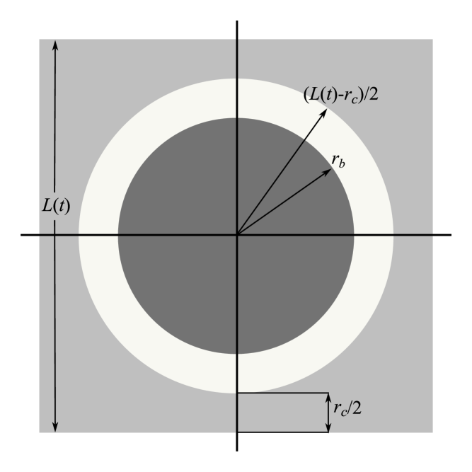
Figure 1: The diagram represents the three regions in the simulation. The inner darker circle represents the Hamiltonian region which is not affected by the barostat or the thermostat and whose diameter is held fixed, the white region is where the function $g(\bm{q},V)$ increases from zero to unity and the outer lighter grey region is where $g(\bm{q},V)$ is set to unity. The minimum width separating the white region from it’s minimum image must be at least as wide as the maximum cutoff radius for the interaction between the particles. The outer boundary of the white region may fluctuate with the volume.

The time dependencies of the multipliers are such that the equilibrium equations of motion preserve the isothermal isobaric distribution function with fixed centre of mass at the origin and zero total momentum:

$$f_{0}(\bm{\Gamma},V)=\frac{\exp(-\beta(H_{0}(\bm{\Gamma})+P_{0}V)\delta(\mathbf{p}_{tot})\delta(\mathbf{R})}{\int_{0}^{\infty}dV\,\int d\bm{\Gamma}\exp(-\beta(H_{0}(\bm{\Gamma})+P_{0}V))\delta(\mathbf{p}_{tot})\delta(\mathbf{R})}.$$ (3)

Here $\mathbf{\Gamma\equiv}\mathbf{(q},\mathbf{p})$, $\beta=1/(k_{B}T_{0})$ where $T_{0}$ is the thermostat temperature, $H_{0}$ is the Hamiltonian associated with the standard Newtonian equations of motion and $P_{0}$ is the externally applied pressure. We note that this approach can be used to produce equations of motion that preserve the isothermal isobaric distribution while only considering configurational variables for the feedback mechanism Braga and Travis (2006). The details of how the distribution function is preserved are given below, resulting in the following time dependencies for the multipliers

$$\dot{\alpha}_{T} = \left(\frac{\sum_{i=1}^{N}g(\mathbf{q}_{i},V)\mathbf{p}_{i}\cdot\mathbf{p}_{i}}{Dmk_{B}T_{0}}-\left[1-\frac{1}{N}\right]\sum_{i=1}^{N}g(\mathbf{q}_{i},V)\right)\frac{1}{\tau_{T}^{2}}$$

$$\dot{\alpha}_{V} = \left(\frac{\sum_{i}^{N}g(\mathbf{q}_{i},V)(\mathbf{p}_{i}\cdot\mathbf{p}_{i}/m+\mathbf{F}_{i}\cdot\mathbf{q}_{i})}{Dk_{B}T_{0}}+\left[1-\frac{1}{N}\right]\frac{1}{D}\sum_{i=1}^{N}\nabla_{i}g(\mathbf{q}_{i},V)\cdot\mathbf{q}_{i}+1-\frac{P_{0}V}{k_{B}T_{0}}+\xi\right)\frac{1}{\tau_{V}^{2}}$$ (4)

where $\tau_{T}\,\&\,\tau_{V}$ are arbitrary time constants and $\xi=\frac{1}{DNk_{B}T}\sum_{i=1}^{N}\sum_{j=1}^{N}g(\bm{\mathbf{q}_{i}},V)\bm{q_{i}\cdot}\bm{F}_{j}$ . Usually the forces all sum to zero $\sum_{j=1}^{N}\bm{F}_{j}=0$ and thus $\xi=0$, however if an external conservative potential is present (the case of a stationary optical trap for example Wang et al. (2002)) then $\xi\neq 0$. Note that as usual, care needs to be taken with the use $\sum_{i}^{N}g(\mathbf{q}_{i},V)\mathbf{F}_{i}\cdot\mathbf{q}{}_{i}$ in a periodic system, and the correct expression for this case is given in the footnote foo (b). The constraints on the system, $\bm{\gamma_{q}}$ and $\bm{\gamma_{p}}$ may be made arbitrarily small by increasing the number of particles in the system or alternatively by choosing the arbitrary time constants $\tau_{T}$ and $\tau_{V}$ to be large while keeping the number of particles in the system fixed. The phase space compression factor, i.e. the divergence of the equations of motion, $\Lambda=\nabla_{\bm{q}}\cdot\dot{\bm{q}}+\nabla_{\bm{p}}\cdot\dot{\bm{p}}+\partial\dot{V}/\partial V+\partial\dot{\alpha}_{T}/\partial\alpha_{T}+\partial\dot{\alpha}_{V}/\partial\alpha_{V}$, is

$$\Lambda=-\alpha_{T}(1-1/N)D\sum_{i=1}^{N}g(\mathbf{q}_{i},V)+\alpha_{V}(1-1/N)\sum_{i=1}^{N}\nabla_{i}g(\mathbf{q}_{i},V)\cdot\mathbf{q}_{i}+\alpha_{V}D,$$ (5)

and the extended Hamiltonian is defined as

$$H_{E}=H_{0}+\frac{D}{2}\alpha_{T}^{2}\tau_{T}^{2}k_{B}T_{0}+\frac{D}{2}\alpha_{V}^{2}\tau_{V}^{2}k_{B}T_{0}.$$ (6)

The extended instantaneous enthalpy is then defined $I_{E}\equiv H_{E}+P_{0}V$. We are now in a position to consider the time-dependence of $f_{0}(\bm{\Gamma},V)$ using the dynamics. We expect an equilibrium distribution function that is consistent with Boltzmann’s postulate of equal a priori probability Eq. 3. A dynamical system in equilibrium has the property that the distribution function for the ensemble is preserved $\partial f(\mathbf{\Gamma},V,t)/\partial t=0$, i.e. it is the time independent solution to the Liouville equation. Using the equations of motion it can be shown that

$$\frac{dI_{E}}{dt}=k_{B}T_{0}\Lambda$$ (7)

and using,

$$\frac{\partial f(\bm{\Gamma},V,t)}{\partial t}=-\dot{\bm{\Gamma}}\cdot\nabla_{\bm{\Gamma}}f(\bm{\Gamma},V,t)-\dot{V}\frac{\partial f(\bm{\Gamma},V,t)}{\partial V}-\Lambda f(\bm{\Gamma},V,t),$$ (8)

it is straightforward to show that this condition is obeyed when the extended distribution function is of the form, $f(\mathbf{\bm{\Gamma}^{\prime}},t)\propto\exp(-\beta I_{E}(\mathbf{\Gamma^{\prime}}))$ where $\mathbf{\Gamma}^{\prime}$ represents the extended phase space vector $\mathbf{\Gamma}^{\prime}\equiv(\mathbf{\bm{\Gamma}},V,\mathbf{\alpha}_{T},\mathbf{\alpha}_{V})$. Thus we obtain the standard isothermal isobaric distribution function with the addition of the two extra independent Nosé Hoover variables,

$$f(\bm{\Gamma}^{\prime}) = f_{0}(\bm{\Gamma},V)\,\frac{D\tau_{T}\tau_{V}}{2\pi}\exp\left(\frac{D}{2}\left(\alpha_{T}^{2}\tau_{T}^{2}+\alpha_{V}^{2}\tau_{V}^{2}\right)\right).$$ (9)

Given the standard isothermal isobaric distribution function, $f_{0}(\bm{\Gamma},V)$, Eq. 3, and assuming the system undergoes a uniform dilation it is easy to prove (i.e. the virial theorem) that at equilibrium,

$$P_{0}=\left\langle\frac{1}{DV(t)}\left(\frac{\sum_{i=1}^{N}\mathbf{p}_{i}\cdot\mathbf{p}_{i}}{m}+\sum_{i=1}^{N-1}\sum_{j=i+1}^{N}\mathbf{F}_{ij}\cdot\mathbf{q}_{ij}\right)\right\rangle$$ (10)

and that the kinetic temperature is given by the equipartition theorem,

$$k_{B}T=\frac{1}{D(N-1)m}\sum_{i=1}^{N}(\mathbf{p}_{i}\mathbf{\cdot}\mathbf{p}_{i}).$$ (11)

So we expect these equations to be obeyed if the above is implemented in a computer simulation.

III Testing For Equilibrium

It is perhaps most effective to test for equilibrium using a small periodic system in two Cartesian dimensions. To do this we will make $r_{b}=0$ , so all particles lie in the reservoir region at all times. So,

$$g(\mathbf{q}_{i},V(t)) = \frac{1}{2}\left(1-\cos\left(2\pi\frac{q_{i}}{L-r_{c}}\right)\right),\;\;\;0<q_{i}<(L-r_{c})/2$$ (12)

$$g(\mathbf{q}_{i},V(t)) = 1,\;\;\;q_{i}>(L-r_{c})/2,$$

where $L=V^{1/D}$ and periodic boundary conditions are used foo (b).

We set the multipliers $\alpha_{V}=\alpha_{T}=4$, with the Cartesian dimension $D=2$, the number of particles $N=36$ and used the WCA potential Weeks et al. (1971) with the Lennard Jones $\sigma$ and $\epsilon$ parameters set to unity and the potential cutoff radius coinciding with $r_{c}$ in Eq. 12. Two simulation sets were computed, firstly at the pressure $P_{0}=0.5$ and temperature $T_{0}=1$, then at the pressure $P_{0}=3.5$ and temperature $T_{0}=4$. The equations Eq. 10 and Eq. 11 were used to obtain the average pressure and temperature. At the two state points averages were calculated for $10^{5}$ time steps with $dt=0.001$ using a $4th$ order Runge-Kutta integrator Butcher and Wanner (1996). This was repeated $50$ times and the standard error was calculated. The results are shown in Table 1. The difference between the input parameters and the averages is consistent with the standard error for the four variables. This provides strong evidence that the analysis we have presented so far is indeed correct.

$P_{0}$	Eq. 10	S.E.	$T$	Eq. 11	S.E.
0.5	0.50002	0.0003	1	1.0006	0.001
3.5	3.5001	0.0015	4	3.9970	0.003

Table 1: The average values obtained for the pressure and the temperature along with the standard error for a system with 36 particles in 2 dimensions.

IV The Crooks Fluctuation Theorem and the Jarzynski Equality

The CFT Crooks (1998, 1999) gives the probability of observing an amount of work $\Delta W=B$, in transforming a system from an initial equilibrium state $I_{E,1}$ to a final state $I_{E,2}$ (where the system will eventually relax to a new equilibrium), relative to observing the opposite amount of work $\Delta W=-B$ for the reverse process starting from the equilibrium state $I_{E,2}$. The ratio between the likelihood of these two observations is given in terms of the difference in free energy between the two equilibrium states. The JE Jarzynski (1997a, b) gives the change in free energy between two equilibrium states in terms of the ensemble average of the exponential of the amount of work it takes to do the transformation. For both theories the two different equilibrium states must have the same temperature. These theories stand out as important due to the fact that they give differences in equilibrium thermodynamic potentials from nonequilibrium data. They also remain valid arbitrarily far from equilibrium.

The Gibbs free energy is given by,

$$G=-k_{B}T_{0}\ln\Delta(P_{0},T_{0}),$$ (13)

where the partition function $\Delta$ is the normalisation constant for $f_{0}(\bm{\Gamma},V)$ (see Eq. 3) and thus,

$$G=-k_{B}T_{0}\ln\left[\int_{0}^{\infty}dV\int d\bm{\Gamma}\delta(\mathbf{p}_{tot})\delta(\mathbf{R})\exp[-\beta(H_{0}(\bm{\Gamma})+P_{0}V)]\right].$$ (14)

A natural definition of the rate of work (here the system’s temperature $T_{0}$ is held fixed) done on the system can be obtained by considering the first law of thermodynamics,

$$\frac{dw_{t}}{dt}=\frac{\partial I_{E}(\bm{\Gamma}^{\prime},t)}{\partial t}=\frac{dI_{E}(\bm{\Gamma}^{\prime}(t),t)}{dt}-k_{B}T_{0}\Lambda,$$ (15)

where the time dependence in the instantaneous enthalpy $I_{E}$ is due to a parametric change, i.e. $I_{E}(\bm{\Gamma}^{\prime},t)=I_{E}(\bm{\Gamma}^{\prime},\lambda(t))$ in the Hamiltonian for the system. This definition remains useful when the parametric change alters the pressure $P_{0}$. If the time dependence is solely due to changing the pressure $P_{0}$ then Eq. 15 gives $\dot{w}_{t}=V\>dP_{0}(t)/dt$. Of course if $P_{0}$ is parametrically changed the blanketing technique is no longer able to circumvent thermostatting artefacts. At time $t=0$ the system is in an initial equilibrium with $I_{E}(\bm{\Gamma}^{\prime},0)=I_{E,1}(\bm{\Gamma}^{\prime})$, the system then undergoes some transformation during the time interval $0<t<\tau$ and then for times $t>\tau$ the system relaxes to a new equilibrium, $I_{E}(\bm{\Gamma}^{\prime},t>\tau)=I_{E,2}(\bm{\Gamma}^{\prime})$, which is reached at the sufficiently later time $t_{f}\gg\tau$. We need to calculate the probability of observing a certain amount of work done on the system in transforming it from an initial equilibrium with $I_{E,1}$ compared to the opposite amount of work when the system undergoes the same transformation in reverse from an initial equilibrium with $I_{E,2}$. We consider an ensemble of trajectories, the number of which approaches infinity. Following the procedure exploited in the derivation of the Evans Searles fluctuation theorem Evans and Searles (1994, 2002), the probability of observing a trajectory with selected values of a property, such as work, can be obtained by summing over the product of the distribution function and the phase volume $\delta V_{\bm{\Gamma}}$ for trajectories that satisfy the selection criterion. Hence, the probability ratio between the forward and reverse process is,

$$\frac{p_{f}(w_{\tau}=B)}{p_{r}(w_{\tau}=-B)}=\frac{\sum_{\bm{\Gamma}(0)|w_{\tau}=B,dB}\delta V_{\bm{\Gamma}}(\bm{\Gamma^{\prime}}(0))f_{1}(\bm{\Gamma^{\prime}}(0))}{\sum_{\bm{\Gamma}(0)|w_{\tau}=B,dB}\delta V_{\bm{\Gamma}}(\bm{\Gamma^{\prime,T}}(\tau))f_{2}(,\bm{\Gamma}^{\prime T}(\tau))]},$$ (16)

where $f_{1}$ is the distribution function for state 1 and $f_{2}$ for state 2, the vector $\bm{\Gamma}^{\prime,T}$ represents the time reversal transformation of $\bm{\Gamma}^{\prime}$ (which has a unit Jacobian) i.e. $\bm{p}\rightarrow-\bm{p}$, $\alpha_{V}\rightarrow-\alpha_{V}$ and $\alpha_{T}\rightarrow-\alpha_{T}$, and $\delta V(\bm{\Gamma}^{\prime}(0))$ is the hyper-volume element in extended phase space surrounding the trajectory bundle. The summation is over all trajectory bundles which result in the amount of work done by the complete transformation process being in the range $w_{\tau}=B\pm dB/2$. It is also assumed here, and below, that all $\bm{\Gamma}$ lie on the $\mathbf{p}_{tot}=\mathbf{0}$ and $\mathbf{q}_{cm}=\mathbf{0}$ hypersurface. For the particular case here, using the equations of motion Eq. 1 this becomes,

$$\frac{p_{f}(w_{\tau}=B)}{p_{r}(w_{\tau}=-B)} = \frac{\sum_{\bm{\Gamma}^{\prime}(0)|w_{\tau}=B,dB}\delta V_{\bm{\Gamma}}(\bm{\Gamma}^{\prime}(0))\exp[-\beta I_{E,1}(\bm{\Gamma}^{\prime}(0))]}{\sum_{\bm{\Gamma}^{\prime}(0)|w_{\tau}=B,dB}\delta V_{\bm{\Gamma}}(\bm{\Gamma}^{\prime,T}(\tau))\exp[-\beta(I_{E,2}(\bm{\Gamma}^{\prime,T}(\tau))]}\frac{\exp(\beta G_{1})}{\exp(\beta G_{2})},$$ (17)

The quantities $G_{1}$ and $G_{2}$ are calculated from Eq. 14 with $I_{E}(\bm{\Gamma}^{\prime})$ given by either $I_{E,1}(\bm{\Gamma}^{\prime})$ or $I_{E,2}(\bm{\Gamma}^{\prime})$. The first law of thermodynamics manifests itself in Eq. 15 and thus the rate at which heat is exchanged with the reservoir is given by $k_{B}T\Lambda$. The probability distribution, in the streaming representation, starting from an initial distribution at time $t=0$ may be obtained from the streaming Liouville equation Evans and Searles (1995, 2002) and is

$$f(\bm{\Gamma}^{\prime}(t),t)=f(\bm{\Gamma}^{\prime}(0),0)\exp\left(-\int_{0}^{t}ds\,\Lambda(\bm{\Gamma}^{\prime}(s))\right).$$ (18)

If we consider a packet of trajectories initially contained by the infinitesimal element of volume $\delta V(\bm{\Gamma}^{\prime}(0))$ we may later observe them contained by the infinitesimal element of volume $\delta V(\bm{\Gamma}^{\prime}(t))$ . By construction, the number of trajectories, or ensemble members, in these two infinitesimal elements is conserved and thus we have

$$\delta V(\bm{\Gamma}^{\prime}(t))f(\bm{\Gamma}^{\prime}(t))=\delta V(\bm{\Gamma}^{\prime}(0))f(\bm{\Gamma}^{\prime}(0))$$ (19)

and in turn

$$\delta V(\bm{\Gamma}^{\prime}(t))=\delta V(\bm{\Gamma}^{\prime}(0))\exp\left(\int_{0}^{t}ds\,\Lambda(\bm{\Gamma}^{\prime}(s))\right)$$ (20)

Now by the first law Eq. 15 we have $I_{E}(\tau)=I_{E}(0)+w_{\tau}+k_{B}T\int_{0}^{t}ds\,\Lambda(\bm{\Gamma}^{\prime}(s))$: substituting this into the denominator of Eq. 17 along with Eq. 20 and noting $I_{E}(\bm{\Gamma}^{\prime,T})=I_{E}(\bm{\Gamma}^{\prime})$ gives,

$$\frac{p_{f}(w_{\tau}=B)}{p_{r}(w_{\tau}=-B)}=\frac{\sum_{\bm{\Gamma}^{\prime}(0)|w_{\tau}=B,dB}\delta V(\bm{\Gamma}^{\prime}(0))\exp[-\beta I_{E,1}(\bm{\Gamma}^{\prime}(0))]}{\sum_{\bm{\Gamma}^{\prime}(0)|w_{\tau}=B,dB}\delta V(\bm{\Gamma}^{\prime}(0))\exp[-\beta(I_{E,1}(\bm{\Gamma}^{\prime}(0))+w_{\tau})]}\exp(-\beta\Delta G)$$ (21)

where $\Delta G=G_{2}-G_{1}$. Thus we obtain the CFT in the isothermal isobaric ensemble,

$$\frac{p_{f}(w_{\tau}=B)}{p_{r}(w_{\tau}=-B)}=\exp[-\beta(\Delta G-B)]$$ (22)

which gives the probability of observing the amount of work $w_{\tau}=B$ done in the transformation process from initial equilibrium state $I_{E,1}$ relative to the probability of observing the amount of work $w_{\tau}=-B$ for the reverse process starting from an initial equilibrium state $I_{E,2}$. It is now trivial to integrate Eq. 22,

$$\int_{-\infty}^{\infty}dB\,p_{f}(w_{\tau}=B)\exp[-\beta B]=\exp[-\beta\Delta G]\int_{-\infty}^{\infty}dB\,p_{r}(w_{\tau}=-B)$$ (23)

and arrive at the JE

$$\left\langle\exp[-\beta w_{\tau}]\right\rangle=\exp[-\beta\Delta G].$$ (24)

Thus by taking the ensemble average of the exponential of the work done (defined through Eq. 15) in transforming the system we obtain the change in Gibbs free energy $\Delta G$. We again point out that this derivation, which starts from the basic equations of motion, has been carried out for a system of interest governed by the fundamental Newtonian equations of motion. This is only possible because the equations of motion we have introduced here allow us to in effect decouple the Newtonian system of interest from the larger thermal reservoir and take advantage of the principle of locality. This proof is valid far from equilibrium as opposed to existing stochastic proofs for the isothermal isobaric ensemble Park and Schulten (2004) which are only valid for Markovian systems.

The JE and CFT provide practical approaches for obtaining $\Delta G$ by measuring the work done along an ensemble of nonequilibrium paths that transform the system from one state to another. However since the derivation of Eq. 24 is reliant on the specification of the equilibrium distribution function, numerical verification of this equation is also an indication that the distribution function indicated in Eq. 9 is actually generated by the equilibrium equations of motion.

V Demonstration: Stretching a Crude Polymer Model

Figure 2: The solid line is the change in Gibbs free energy as a function of distance between the two traps $l_{tr}$ calculated from a series of equilibrium simulations using Eq. 27. The diamonds are the work done in stretching the polymer at a finite rate and the circles are the results obtained from the JE, Eq. 24.

To form a crude model of a single polymer suspended in a solvent of Cartesian dimension $D=2$ we use the finite extendable nonlinear elastic (FENE) chain model Kröger (2004). The two end particles of the polymer are held by a pair of harmonic wells $U_{h}(x)=\frac{1}{2}k_{t}x^{2}$, i.e. as in optical traps Wang et al. (2002). We may then apply the JE to the case where the polymer is stretched due to the two traps being moved apart. We note that previous work has addressed how to determine the free energy difference as a function of the polymer separation rather than the trap separation Hummer and Szabo (2005). All particles, solvent and polymer, interact by the same repulsive WCA potential Weeks et al. (1971) and have the same mass. In addition neighbouring polymer particles are bound together by the FENE potential Kröger (2004)

$$U_{FENE}=-\frac{1}{2}Kr_{0}^{2}\ln\left[1-(\Delta r/r_{0})^{2}\right],$$ (25)

where the particles must be separated by a distance $\Delta r$ which is less than $r_{0}$ where the potential diverges and $K$ is the strength of the potential. The spatial derivative gives us the force

$$F_{FENE}=-\nabla U_{FENE}=-K\Delta\mathbf{r}/\left(1-(\Delta r/r_{0})^{2}\right).$$ (26)

We set the FENE parameters to $K=10\epsilon$ and $r_{0}=1.5\sigma$ where $\epsilon$ and $\sigma$ are the parameters from the WCA potential. The total number of particles is $N=300$, the number of polymer particles is $N_{p}=8$, the trap strength is $k_{t}=2\epsilon/\sigma^{2}$, the temperature is $T=\epsilon/k_{B}$ were $k_{B}$ is Boltzmann’s constant and the pressure is $P_{0}=2\sigma^{2}/\epsilon$. The time is reported in units of $\sigma\sqrt{m/\epsilon}$ where $m$ is the particle mass and lengths are reported in units of $\sigma$. The optical traps where initially set at a separation distance of $l_{tr}=2.5$ and stretched to a distance of $l_{tr}=6.5$. With $l_{tr}=2.5$ the average volume was found to be $\left\langle V\right\rangle=521.9\pm 0.2$ and with $l_{tr}=6.5$, $\left\langle V\right\rangle=522.3\pm 0.2$, where the figure in the error estimate is one standard error. The traps were centred abound the Newtonian region in the simulation. In the spirit of the method originally introduced by Hoover and Ree Hoover and Ree (1968) the average equilibrium length of the polymer $l_{p}$, in the direction of the vector connecting the two traps, was computed for $31$ separation distances between and including the shortest and longest length. This data was then used to compute the equilibrium change in Gibbs free energy using the equation

$$\frac{dG}{dl_{tr}}=-\frac{1}{2}k_{tr}\left(l_{p}-l_{tr}\right),$$ (27)

with the trapezoidal quadrature. For the JE the work for Eq. 24 obtained from Eq. 15 is computed from the equation

$$\frac{dw_{t}}{dt}=-\frac{1}{2}k_{tr}\frac{dl_{t}}{dt}\left(x_{p,r}-x_{p,l}-l_{tr}\right),$$ (28)

where $x_{p,r}$ is the $x$ component of the position of the particle at the right hand end of the polymer and $x_{p,l}$ that at the left hand end. Both traps are located on the $x$ axis.

A total of $5\times 10^{4}$ nonequilibrium trajectories were computed starting from equilibrium with $l_{tr}=2.5$ and stretched at a constant rate until $l_{tr}=6.5$ over a duration of $\tau=100$. The results may be seen in Fig. 2. The average work done in the nonequilibrium stretching of the polymer is clearly greater than the change in free energy indicating that energy is being irreversibly dissipated into the thermal reservoir. It can be seen, despite the irreversible work, that there is excellent agreement between the change in free energy calculated using equilibrium methods Eq. 27 and the change in free energy calculated using the JE Eqs. 24 & 28.

VI Conclusions

We have introduced equations of motion that preserve the isothermal isobaric ensemble’s distribution function yet still feature a region which is governed by the natural Newtonian equations of motion. This natural region can be chosen to be arbitrarily large. As we have argued previously Evans and Searles (2002); Williams et al. (2004) if the thermostatted, barostatted blanket is far enough removed (from the system of interest) its details can not possibly effect the physical observations made in the system of interest. This amounts to the assumption of locality, which is one of the most important and well established assumptions in physics. When a far from equilibrium process occurs in the system of interest the heat flux which is dissipated into the outer blanket diminishes with distance: for $D=3$ this will be proportional to the inverse square of the distance. If the blanket is far enough removed from the system of interest the thermostat and barostat will only act on a region that is in local equilibrium and it is known that this class of thermostatted dynamics does not introduce any artifacts when in local equilibrium Evans and Morriss (1990).

In the arrangement described here, the system of interest is in a spherical region. Other physical arrangements could be designed, for example it could be a slit shaped region. This arrangement would be more useful for studying some nonequilibrium steady state dynamics (e.g. Poiseuille flow).

Using these equations of motion we have derived the CFT and the JE in the isothermal isobaric ensemble that will be applicable regardless of how far from equilibrium the system of interest is driven. The only physical assumption necessary for this is the assumption of locality. Existing derivations for the isothermal isobaric ensemble using Markovian stochastic dynamics Park and Schulten (2004), can only be linked to the fundamental microscopic equations, at best, in the near equilibrium linear response regime. One of the remarkable features of these theories is that they remain valid far from equilibrium. We now have a proofs of the JE and the CFT that remain valid far from equilibrium in the isothermal isobaric ensemble. It is this ensemble, with the Gibbs free energy as the thermodynamic potential, which is most relevant to physical experiments and processes.