Simple implementation of complex functionals: scaled selfconsistency

Abstract

We explore and compare three approximate schemes allowing simple implementation of complex density functionals by making use of selfconsistent implementation of simpler functionals: (i) post-LDA evaluation of complex functionals at the LDA densities (or those of other simple functionals); (ii) application of a global scaling factor to the potential of the simple functional; and (iii) application of a local scaling factor to that potential. Option (i) is a common choice in density-functional calculations. Option (ii) was recently proposed by Cafiero and Gonzalez. We here put their proposal on a more rigorous basis, by deriving it, and explaining why it works, directly from the theorems of density-functional theory. Option (iii) is proposed here for the first time. We provide detailed comparisons of the three approaches among each other and with fully selfconsistent implementations for Hartree, local-density, generalized-gradient, self-interaction corrected, and meta-generalized-gradient approximations, for atoms, ions, quantum wells and model Hamiltonians. Scaled approaches turn out to be, on average, better than post-approaches, and unlike these also provide corrections to eigenvalues and orbitals. Scaled selfconsistency thus opens the possibility of efficient and reliable implementation of density functionals of hitherto unprecedented complexity.

I Introduction

Density-functional theory kohnrmp ; dftbook ; parryang is the driving force behind much of todays progress in electronic-structure calculations. Progress in density-functional theory (DFT) itself depends on the twin development of ever more precise density functionals and of ever more efficient computational implementations of these functionals. The first line of development, functionals, has lead from the local-density approximation (LDA) to generalized-gradient approximations (GGAs), hybrid functionals, and on to meta-GGAs and other fully nonlocal approximations, such as exact-exchange (EXX) and self-interaction corrections (SICs).perdewreview ; oepreview

As functionals get more and more complex, the second task, implementation, gets harder and harder. Indeed, very few truly selfconsistent implementations of beyond-GGA functionals exist, and even GGAs are still sometimes implemented non-selfconsistently. At the heart of the problem is not so much the actual coding (although that can also be a formidable task, considering the complexity of, e.g., meta-GGAs), but rather obtaining the exchange-correlation ($xc$) potential $v_{xc}({\bf r})$ corresponding to a given approximation to the $xc$ energy $E_{xc}[n]$. Hybrid functionals, meta-GGAs, EXX and SICs are all orbital functionals, i.e., functionals of the general form $E^{orb}_{xc}[\{\varphi_{i}[n]\}]$, where our notation indicates an explicit dependence on the set of Kohn-Sham (KS) orbitals $\varphi_{i}({\bf r})$. This set may be restricted to the occupied orbitals, but may also include unoccupied orbitals. Since by virtue of the Hohenberg-Kohn (HK) theorem these orbitals themselves are density functionals, any explicit orbital functional is an implicit density functional.

The HK theorem itself, however, does not provide any clue how to obtain the $xc$ potentials, i.e., how to calculate the functional derivative

$$v_{xc}[n]({\bf r})=\frac{\delta E_{xc}^{orb}[\{\varphi_{i}\}]}{\delta n({\bf r})}$$ (1)

of a functional whose density dependence is not known explicitly. Three different solutions to this dilemma have been advanced in the literature.

(i) The formally correct way to implement an implicit density functional in DFT is the optimized-effective potential (OEP) algorithmoepreview [also known as the optimized potential method (OPM)], which results in an integral equation for the KS potential corresponding to the orbital functional. The first step of the derivation of the OEP is to write

$$v_{xc}[n]({\bf r})=\frac{\delta E_{xc}^{orb}[\{\varphi_{i}\}]}{\delta n({\bf r})}$$ (2)

$$=\int d^{3}r^{\prime}\sum_{i}\left[\frac{\delta E_{xc}^{orb}[\{\varphi_{i}\}]}{\delta\varphi_{i}({\bf r^{\prime}})}\frac{\delta\varphi_{i}({\bf r^{\prime}})}{\delta n({\bf r})}+c.c.\right]$$ (3)

$$=\int d^{3}r^{\prime}d^{3}r^{\prime\prime}\sum_{i}\left[\frac{\delta E_{xc}^{orb}[\{\varphi_{i}\}]}{\delta\varphi_{i}({\bf r^{\prime}})}\frac{\delta\varphi_{i}({\bf r^{\prime}})}{\delta v_{s}({\bf r^{\prime\prime}})}\frac{\delta v_{s}({\bf r^{\prime\prime}})}{\delta n({\bf r})}+c.c.\right].$$ (4)

Further evaluation of Eq. (4) gives rise to an integral equation that determines the $v_{xc}[n]$ belonging to the chosen orbital functional $E^{orb}_{xc}[\{\varphi_{i}[n]\}]$. This OEP integral equation must be solved at every step of the selfconsistency cycle, which considerably increases demands on memory and computing time. Often (in particular for systems that do not have spherical symmetry) the integral equation is simplified by means of the Krieger-Li-Iafrate (KLI) approximation,kli but even within this approximation, or other recently proposed simplifications,kuemmelperdew ; wuyang an OEP calculation is computationally more expensive than a traditional KS calculation. A separate issue is the unexpected behaviour of the OEP in finite basis sets, which was recently reported to cast doubt on the reliability of the method.staroverov The OEP prescription moreover assumes in the first step that the orbital derivative $\delta E_{xc}^{orb}[\{\varphi_{i}\}]/\delta\varphi_{i}({\bf r^{\prime}})$ can be obtained, and even that is not a trivial task for complex orbital-dependent functionals such as meta-GGA and hyper-GGA. (For the Fock term, on the other hand, this derivative is simple, and the implementation of the Fock term by means of the OEP is becoming popular under the name exact exchange [EXX]).

(ii) Instead of taking the variation of $E_{xc}[\{\varphi_{i}[n]\}]$ with respect to $n({\bf r})$, as in the OEP, one often makes $E_{xc}$ stationary with respect to the orbitals. When applied to the Fock term, this is simply the Hartree-Fock (HF) method, but similar procedures are commonly applied within DFT to hybrid functionals, such as B3-LYP. Selfconsistent implementations of meta-GGA reported until today are also selfconsistent with respect to the orbitals, not the densities.handymgga ; mggatests1 ; mggatests2 For the Fock term, one finds empirically that the occupied orbitals obtained from orbital selfconsistency are quite similar to those obtained from density selfconsistency, but such empirical finding is no guarantee that the similarity will persist for all possible functionals or systems — and in any case it does not extend to the unoccupied orbitals. Computationally, the resulting nonlocal HF-like potential makes the solution of the Kohn-Sham equation more complex than the local potential resulting from the OEP (although the potential itself is obtained in a simpler way). Moreover, as the OEP, this prescription also requires that the orbital derivative $\delta E_{xc}^{orb}[\{\varphi_{i}\}]/\delta\varphi_{i}({\bf r^{\prime}})$ can be obtained, which need not be simple for complex functionals.

(iii) Less demanding than density-selfconsistency or orbital-selfconsistency are post-selfconsistent implementations, in which a selfconsistent KS calculation is performed with a simpler functional, and the resulting orbitals and densities are once substituted in the more complex one. This strategy is sometimes used to implement GGAs in a post-LDA way, and has been applied also to meta-GGAs. It is much simpler than the other two possibilities, but does not lead to KS potentials, orbitals, and single-particle energies associated with the complex functional. It simply yields the total energy the complex functional produces on the densities obtained from the simpler functional.

As this brief summary shows, each of the three choices has its own distinct set of advantages and disadvantages. A method that is simple to implement, reliable, and provides access to total energies as well as single-particle quantities would be a most useful addition to the arsenal of computational DFT.

A method we consider to have the desired characteristics was recently proposed by Cafiero and Gonzalez,cafiero and consists in the application of a scaling factor to the $xc$ potential of a simple functional (which can be implemented fully selfconsistently), such that it approximates the potential expected to arise from a complex functional (which need not be implemented selfconsistently). This fourth possibility, which we call globally-scaled selfconsistency (GSSC), is analysed in Sec. II of the present paper.

We believe the derivation presented by Cafiero and Gonzalez to lack rigour at a crucial step, and thus dedicate Sec. II.1 to an investigation of their procedure. Our investigation leads to an alternative derivation of the same approach, described in Sec. II.2. Next, we provide, in Sec. II.3, an analysis of the validity of the scaling approximation, arriving at the counterintuitive (but numerically confirmed and explainable) conclusion that the success of this approximation is not due to the smallness of the neglected term relative to the one kept. We also suggest a modification of the approach, which we call locally-scaled selfconsistency (LSSC) and describe in Sec. II.4.

In Secs. III and IV we provide extensive numerical tests of GSSC and LSSC, and also of the more common post-selfconsistent mode of implementation [here denoted P-SC, option (iii) above]. Note that although P-SC is quite commonly used, it has not been systematically tested in situations where the exact result or the fully selfconsistent result is known. All three schemes are applied to atoms and ions in Secs. III.1 and III.2, to one-dimensional Hubbard chains, in Sec. IV.1, and to semiconductor quantum wells, in Sec. IV.2. We compare Hartree, LDA, GGA, MGGA and SIC calculations, implemented via P-SC, GSSC and LSSC, among each other, and, where possible, with results obtained from fully selfconsistent implementations of the same functionals.

Our main conclusion is that scaled selfconsistency works surprisingly well, for all different combinations of systems and functionals we tried. Scaled selfconsistency yields better energies than post-selfconsistent implementations, and moreover provides access to orbitals and eigenvalues. This conclusion opens the possibility of efficient and reliable implementation of density functionals of hitherto unprecedented complexity.

II Scaled selfconsistency

In this section we first briefly review the approach suggested by Cafiero and Gonzalez (CG),cafiero and point out where we believe their development to lack rigour. Next we present an alternative derivation and suggest a modification.

II.1 The proposal of Cafiero and Gonzalez

CG consider a complex functional, $E_{xc}^{B}[n]$ with potential $v_{xc}^{B}({\bf r})$, and a simple functional, $E_{xc}^{A}[n]$ with potential $v_{xc}^{A}({\bf r})$. They then define the energy ratio

$$F_{xc}[n]=\frac{E_{xc}^{B}[n]}{E_{xc}^{A}[n]}$$ (5)

and differentiate $E_{xc}^{B}[n]=F_{xc}[n]E_{xc}^{A}[n]$ with respect to the density $n({\bf r})$, obtaining, in their notation,

$$v_{xc}^{B}({\bf r})=F_{xc}[n]v_{xc}^{A}({\bf r})+E_{xc}^{A}[n]\frac{\partial F_{xc}[n]}{\partial n({\bf r})}.$$ (6)

Next, CG argue that at the selfconsistent density, $n^{*}$, $E_{xc}^{B}[n^{*}]=E_{xc}^{A}[n^{*}]$, so that $F_{xc}[n^{*}]\to 1$. According to CG, the last term in Eq. (6) is then equal to zero. Under this ’constraint’cafiero they obtain

$$v_{xc}^{B}({\bf r})=F_{xc}[n]v_{xc}^{A}({\bf r})$$ (7)

which implies that an (approximate) selfconsistent implementation of the complicated functional $E_{xc}^{B}[n]$ can be achieved by means of a selfconsistent implementation of the simple functional $E_{xc}^{A}[n]$, if at every step of the selfconsistency cycle the potential corresponding to functional A is multiplied by the ratio of the energies of B and A. This procedure completely avoids the need to ever calculate or implement the potential corresponding to $B$. CG go on to test their proposal for a few functionals and systems, and claim very good numerical agreement between approximate results obtained from (7) and fully selfconsistent or post-selfconsistent implementations.

We were initially quite surprised by these good results, as the preceding argument lacks rigour at a key step. Apart from the use of partial derivatives instead of variational ones (which is probably just a question of notation), we do not see why at the selfconsistent density the simple and the complex functional must approach the same value, i.e., why $F[n^{*}]$ should approach one. Moreover, whatever value $F$ approaches, this value should not be used to simplify the equation for the $xc$ potential because the derivative must be carried out before substituting numerical values in the energy functional, not afterwards.

II.2 An alternative derivation

In view of these troublesome features of the original derivation we below present an alternative rationale for the same approach. We start by writing the same identity the CG approach is based on,

$$E^{B}[n]=\frac{E^{B}[n]}{E^{A}[n]}E^{A}[n]=:F[n]E^{A}[n].$$ (8)

Note that we write this identity for an arbitrary energy functional, as the approach is, in principle, not limited to $xc$ functionals. Indeed, below we will show one application in which we deal with the entire interaction energy (Hartree + $xc$). Next, we take the functional derivative of the product $F[n]E^{A}[n]$,

$$v^{B}({\bf r})\equiv\frac{\delta E^{B}[n]}{\delta n({\bf r})}=\frac{\delta F[n]}{\delta n({\bf r})}E^{A}[n]+F[n]\frac{\delta E^{A}[n]}{\delta n({\bf r})}$$ (9)

$$=\frac{\delta F[n]}{\delta n({\bf r})}E^{A}+F[n]v^{A}({\bf r}).$$ (10)

The functional derivative of the ratio $F[n]$ is

$$\frac{\delta}{\delta n({\bf r})}\frac{E^{B}}{E^{A}}=\frac{E^{A}[n]v^{B}({\bf r})-E^{B}[n]v^{A}({\bf r})}{E^{A}[n]^{2}}.$$ (11)

Substitution of this in the previous equation yields the identity

$$v^{B}({\bf r})=\frac{E^{A}[n]v^{B}({\bf r})-E^{B}[n]v^{A}({\bf r})}{E^{A}[n]}+F[n]v^{A}({\bf r}).$$ (12)

Neglecting the first term leaves us with the simple expression

$$v^{B}({\bf r})\approx v^{GSSC}({\bf r}):=F[n]v^{A}({\bf r})$$ (13)

as an approximation to $v^{B}$. In the following this approximation is called globally scaled selfconsistency (GSSC). Scaling here refers to the multiplication of the simple potential $v^{A}({\bf r})$ by the energy ratio $F[n]$ in order to simulate the more complex potential $v^{B}({\bf r})$, and the specifier globally is employed in anticipation of a local variant developed in Sec. II.4.

II.3 Validity of scaled selfconsistency

The form of Eq.(12) suggests a simple explanation of why scaled selfconsistency can lead to results close to those obtained from a fully selfconsistent implementation of functional B: Clearly, $v^{GSSC}({\bf r})$ is a good approximation to $v^{B}({\bf r})$ if the first term in (12) can be neglected compared to the second. Globally scaled selfconsistency is thus guaranteed to be valid if the validity criterium

$$C_{1}({\bf r}):=\frac{\left|E^{A}[n]v^{B}({\bf r})-E^{B}[n]v^{A}({\bf r})\right|}{|E^{B}[n]v^{A}({\bf r})|}<<1$$ (14)

is satisfied at all points in space. Note that this is conceptually a very different requirement from $F[n^{*}]\to 1$, although it leads to the same final result.

Interestingly, criterium (14) is a sufficient, but not at all a necessary, criterium for applicability of the GSSC approach. In fact, in the applications reported below we have frequently encountered situations in which the first term on the right-hand side in Eq. (12) is not much smaller, but comparable to, or even larger than, the second term. The empirical success of scaled selfconsistency, claimed in Ref. cafiero, and confirmed below for a wide variety of functionals and systems, must thus have another explanation, rooted in systematic error cancellation.

One source of error cancellation is the fact that Eq. (14) is a point-wise equation, which, in principle, must be satisfied for every value of ${\bf r}$. For the calculation of integrated quantities (such as total energies) or quantities determined by the values of $v^{B}({\bf r})$ at all points in space (such as KS eigenvalues) a violation of (14) at some point in space can be compensated by that at some other point. We have numerically verified that this indeed happens: the sign of the term neglected in GSSC can be different in different regions of space, reducing the integrated error.

The extent to which errors at different points cancel in the application of the scaling factor can be estimated by replacing Eq. (14) by

$$C_{2}:=\frac{\int d^{3}r\,E^{A}[n]v^{B}({\bf r})-E^{B}[n]v^{A}({\bf r})}{\int d^{3}rE^{B}[n]v^{A}({\bf r})}<<1.$$ (15)

Representative values of $C_{2}$ are also reported below.

In applications we have frequently obtained excellent total energies even in situations in which this criterium also fails. A second source of error cancellation is the DFT total-energy expression

$$E_{0}[n]=\sum_{i}\epsilon_{i}-E_{H}[n]-\int d^{3}r\,n({\bf r})v_{xc}({\bf r})+E_{xc}[n],$$ (16)

where, ideally, $v_{xc}$ is the functional derivative of $E_{xc}[n]$. Scaled selfconsistency is applied in situations in which $E_{xc}[n]$ is known, but $v_{xc}$ is hard to obtain or to implement. Hence it replaces $v_{xc}$ by $v_{xc}^{GSSC}$ in the second-to-last term, but the last term is evaluated using the original $E_{xc}$. The entire expression is evaluated on the selfconsistent density arising from a Kohn-Sham calculation with potential $v_{xc}^{GSSC}$. In situations in which all terms in (16) can be obtained exactly, we have verified numerically that the errors arising from different terms in the GSSC total energy make contributions of similar size but opposite sign to the total error. Representative analyses of this type are given below.

Numerical comparison of the exact equation (12) and its approximation (13) with results obtained from the local (14) or the integrated (15) validity criterium, and with the errors of each term in the total-energy expression (16), permits us to identify the reason for the success of GSSC. Anticipating results presented in detail in later sections, we find that the excellent approximations to total energies obtained from the simple scaling approach are to a large extent due to the error cancellation between different terms of the total energy, and depend only very weakly on the smallness of the neglected term relative to the one kept.

We end this discussion of validity and errors by pointing out that although frequently a violation of the criteria (14) or (15) still provides good energies, we have never observed the opposite situation, i.e., bad energies in situations in which (14) or (15) are satisfied.

II.4 Locally-scaled selfconsistency

As a result of the previous section, we have the expression

$$v^{B}[n]({\bf r})\approx$$

$$v^{GSSC}[n]({\bf r})=\frac{E^{B}[n]}{E^{A}[n]}v^{A}[n]({\bf r})=F[n]v^{A}[n]({\bf r})$$ (17)

for globally-scaled selfconsistency. Note that the scaling factor depends on the density, i.e., is updated in every iteration of the selfconsistency cycle, but does not depend on the spatial coordinate ${\bf r}$, i.e., is the same for all points in space.

Clearly, such a global scaling factor cannot properly account for the fine point-by-point differences expected between the potentials $v^{A}({\bf r})$ and $v^{B}({\bf r})$. In an attempt to account for these differences, we introduce a local scaling factor, based on the observation that many functionals (in particular, LDA, GGA and MGGA) can be cast in the form

$$E[n]=\int d^{3}r\,e(n(r)),$$ (18)

where the energy density $e(n)$ is defined (up to a total divergence) by the above expression, and the dependence of $e(n)$ on $n({\bf r})$ may be both explicit (as in LDA) or implicit (as in meta-GGA). The energy density allows us to introduce a local scaling factor $f[n]({\bf r})$, according to

$$v^{B}[n]({\bf r})\approx v^{LSSC}[n]({\bf r})=$$ (19)

$$\frac{e^{B}[n]({\bf r})}{e^{A}[n]({\bf r})}v^{A}[n]({\bf r})=:f[n]({\bf r})v^{A}[n]({\bf r}).$$ (20)

In the applications below we refer to $v^{GSSC}[n]$ as the globally scaled potential (with upper-case scaling factor $F$), and to $v^{LSSC}$ as locally scaled potential (with lower-case scaling factor $f({\bf r})$).

We also explored a variety of alternative scaling schemes, such as, e.g., application of scaling factors to the full effective potential instead of just its $xc$ contribution, or directly to the density. None of these consistently led to better results than the GSSC and LSCC procedures, and we refrain from presenting detailed results from alternative schemes here.

III Tests and applications to atoms and ions

In this section we compare post-selfconsistent implementations and globally and locally scaled implementations of different density functionals for total energies and Kohn-Sham eigenvalues of atoms and ions. We provide comparisons of these modes of implementation among each other and, where possible, with fully selfconsistent applications. We also provide representative evaluations of the validity criteria discussed in Sec. II.3.

III.1 Total energy of atoms and ions: LDA, GGA, Meta-GGA and SIC

Ground-state energies of neutral atoms from $Z=2$ to $Z=18$ are shown in Tables 1 to 3. In Table 1 we compare selfconsistent LDA(PZpz81 ) and GGA(PBEpbe ) energies with energies obtained by three approximate schemes: post-LDA implementation of GGA and globally and locally scaled selfconsistency. For global scaling we follow our above discussion and use

$$v_{xc}^{GGA(GSSC)}[n]({\bf r})=\frac{E_{xc}^{GGA}[n]}{E_{xc}^{LDA}[n]}v_{xc}^{LDA}[n]({\bf r})$$ (21)

as $xc$ potential, throughout the selfconsistency cycle. For local scaling, the prefactor of $v_{xc}^{LDA}({\bf r})$ is replaced by the corresponding energy densities. Although GGAs are nowadays often implemented fully selfconsistency, application of approximate schemes to GGA is interesting precisely because fully selfconsistent data are available for comparison. Table 1 clearly shows that both approximate schemes provide excellent approximations to the fully selfconsistent values.

Table 1: Ground-state energies of neutral atoms (in Rydberg) obtained selfconsistently with LDA and with GGA, and approximate GGA energies predicted by globally (F) and locally (f) scaled selfconsistency, starting from LDA, and by post-LDA application (P) of GGA.

atom	LDA	F	f	P	GGA
He	-5.6686	-5.7854	-5.7838	-5.7844	-5.7859
Li	-14.6853	-14.9235	-14.9206	-14.9220	-14.9244
Be	-28.8924	-29.2589	-29.2561	-29.2573	-29.2599
B	-48.7037	-49.2089	-49.2057	-49.2075	-49.2108
C	-74.9315	-75.5846	-75.5813	-75.5835	-75.5874
N	-108.258	-109.068	-109.065	-109.067	-109.072
O	-149.042	-149.998	-149.995	-149.998	-150.002
F	-198.217	-199.327	-199.325	-199.327	-199.331
Ne	-256.455	-257.729	-257.726	-257.728	-257.733
Na	-322.881	-324.341	-324.338	-324.340	-324.345
Mg	-398.265	-399.906	-399.903	-399.905	-399.910
Al	-482.628	-484.459	-484.456	-484.458	-484.464
Si	-576.429	-578.458	-578.455	-578.458	-578.464
P	-679.991	-682.225	-682.222	-682.224	-682.231
S	-793.471	-795.886	-795.883	-795.885	-795.892
Cl	-917.327	-919.935	-919.932	-919.934	-919.941
Ar	-1051.876	-1054.686	-1054.682	-1054.685	-1054.692

Next, we consider two alternative choices of energy functionals, for which fully selfconsistent results are not readily available: meta-GGA and self-interaction corrections. In Table 2 we compare a GSCC implementation of meta-GGA(TPSS)tpss1 ; tpss2 with results obtained from a post-GGA(PBE) implementation of the same functional. Fully selfconsistent implementation of meta-GGA would require the OEP algorithm, and has not yet been reported. However, previous tests of meta-GGA suggest that orbital selfconsistency and post-GGA implementation of MGGA give rather similar results, and provide significant improvement on GGA.mggatests1 ; mggatests2 Consistently with these observations, and also with those of Ref. cafiero, (which, however, uses the now obsolete PKZB form of meta-GGA), we find, in Table 2, very close agreement between scaled and post-GGA implementations of TPSS meta-GGA. Systematically, the LSSC energies are a little less negative and the GSCC energies very slightly more negative than post-GGA energies.

Table 2: Ground-state energies of neutral atoms obtained selfconsistently with GGA(PBE), compared to meta-GGA(TPSS) energies predicted by globally (F) and locally (f) scaled selfconsistency, starting from GGA, and by post-GGA calculations (P).

atom	GGA	F	f	P
He	-5.7859	-5.8185	-5.7625	-5.8183
Li	-14.9244	-14.9768	-14.9111	-14.9767
Be	-29.2599	-29.3414	-29.2654	-29.3412
B	-49.2108	-49.3077	-49.2061	-49.3076
C	-75.5874	-75.7091	-75.5768	-75.7089
N	-109.0715	-109.2304	-109.0610	-109.2302
O	-150.0019	-150.1664	-149.9781	-150.1662
F	-199.3313	-199.5190	-199.3022	-199.5188
Ne	-257.7329	-257.9607	-257.7085	-257.9605
Na	-324.3454	-324.5951	-324.3452	-324.5949
Mg	-399.9103	-400.1831	-399.9298	-400.1830
Al	-484.4641	-484.7584	-484.4871	-484.7583
Si	-578.4640	-578.7866	-578.4969	-578.7865
P	-682.2314	-682.5997	-682.2784	-682.5896
S	-795.8921	-796.2723	-795.9499	-796.2722
Cl	-919.9413	-920.3493	-920.0101	-920.3492
Ar	-1054.6923	-1055.1359	-1054.7761	-1055.1359

A different type of density functional is represented by the self-interaction correction (SIC). Although several distinct such corrections have been proposed, we here focus on the best known suggestion, made by Perdew and Zunger in 1981 (PZSIC).pz81 PZSIC provides an orbital-dependent correction of the form

$$E_{xc}^{approx,SIC}[n_{\uparrow},n_{\downarrow}]=$$

$$E_{xc}^{approx}[n_{\uparrow},n_{\downarrow}]-\sum_{i,\sigma}\left(E_{H}[n_{i\sigma}]-E_{xc}^{approx}[n_{i\sigma},0]\right),$$ (22)

which can be applied to any approximate density functional $E_{xc}^{approx}$. Here we chose this functional to be the LDA. The correction terms depend on the partial density of each occupied orbital, $n_{i\sigma}({\bf r})$, and not explicitly on the total density. Hence, selfconsistent implementation should proceed via the OEP.norman Instead, common implementations of PZSIC follow a suggestion made in the original reference,pz81 and vary the energy functional with respect to the orbitals. The resulting single-particle equation is not the usual Kohn-Sham equation, but features an effective potential that is different for each orbital.

In Table 3 we compare energies obtained from solution of this equation with those obtained, in a much simpler way, from applying GSCC to LDA+PZSIC. Very good agreement is achieved. This is even more remarkable as in usual implementations of PZSIC the potentials are different for each orbital, and the resulting orbitals are not orthogonal, whereas in the GSSC implementation the local potential is the same for all orbitals, which are automatically orthogonal. Formally, the GSSC implementation is thus more satisfying than the standard implementation.

Table 3: Ground-state energies of neutral atoms obtained selfconsistently with LDA, and PZSIC energies predicted by globally scaled selfconsistency, starting from LDA, and by post-LDA implementation of PZSIC, all compared to energies obtained from a standard (i.e., orbitally selfconsistent) implementation of LDA+PZSIC.

atom	LDA	F	P	LDA+PZSIC
He	-5.6686	-5.8366	-5.8329	-5.8386
Li	-14.6853	-15.0075	-15.0036	-15.0091
Be	-28.8924	-29.3863	-29.3824	-29.3877
B	-48.7037	-49.3992	-49.3946	-49.4007
C	-74.9315	-75.8573	-75.8520	-75.8592
N	-108.258	-109.442	-109.436	-109.445
O	-149.042	-150.505	-150.497	-150.508
F	-198.217	-199.987	-199.979	-199.991
Ne	-256.455	-258.561	-258.551	-258.565
Na	-322.881	-325.332	-325.324	-325.336
Mg	-398.265	-401.060	-401.053	-401.064
Al	-482.628	-485.769	-485.762	-485.773
Si	-576.429	-579.922	-579.916	-579.926
P	-679.991	-683.843	-683.836	-683.846
S	-793.471	-797.689	-797.683	-797.692
Cl	-917.327	-921.920	-921.914	-921.923
Ar	-1051.876	-1056.850	-1056.850	-1056.854

The analysis of total energies of neutral atoms is summarized in Figure 1, which displays the relative deviation

$$\eta=\frac{\left(E_{ref}-E_{GSSC}\right)}{E_{ref}}$$ (23)

of GSCC from selfconsistent data (GGA), post-GGA data (meta-GGA) and orbitally selfconsistent data (PZSIC).

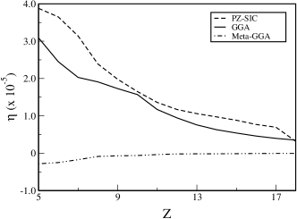
Figure 1: Relative deviation, as defined in Eq. (23), of GSSC GGA compared to selfconsistent GGA (full line), of GSSC meta-GGA compared to post-GGA meta-GGA (dash-dotted line) and of GSCC LDA+PZSIC compared to orbitally selfconsistent LDA+PZSIC. Note that only in the first case this relative deviation can be interpreted as a relative error of GSSC relative to fully selfconsistent results, as in the other two cases different approximations are compared among each other.

Table 4 presents a representative error analysis. Values of $C_{2}$, defined in Eq. (15), indicate that the term neglected in the GSSC approach is smaller than the term kept, but not by a sufficient margin to explain, on its own, the very good approximation to total energies obtained from global scaling. The breakdown of the error of the total energy into the contributions arising from each term individually, shows that there is very substantial error cancellation, mostly between the sum of the KS eigenvalues and the potential energy in the $xc$ potential. As a consequence of this error cancellation, which is ultimately due to the variational principle, selfconsistent total energies are predicted by scaling approaches with much higher accuracy than the values of $C_{2}$ suggest.

Table 4: Breakdown of errors of the different contributions to the total energy in Eq. (16), comparing LDA-based global-scaling predictions of GGA energies (GSSC GGA) with selfconsistent GGA energies. The column labeled $C_{2}$ contains the integrated validity criterium of global scaling, as defined in Eq. (15). Note that we have not defined an integrated validity criterium for local scaling.

atom	$C_{2}$	$\Delta E_{KS}$	$\Delta E_{H}$	$\Delta V_{xc}$	$\Delta E_{xc}$	$\Delta E_{0}$
He	0.016	0.0974	0.0131	0.0766	-0.0081	-0.0004
C	0.115	0.2684	-0.1670	0.4504	0.0122	-0.0028
O	0.016	0.333	-0.318	0.679	0.024	-0.004
Na	0.353	0.464	-0.541	1.041	0.031	-0.004
Si	0.147	0.689	-0.691	1.416	0.030	-0.006
Ar	0.009	0.959	-0.948	1.950	0.036	-0.007

Table 5: Ground-state energies of positive ions, obtained from self-consistent LDA and GGA calculations, as well as from locally and globally scaled LDA calculations.

atom	LDA	F	f	P	GGA
He+	-3.8838	-3.9873	-3.9853	-3.9864	-3.9875
Li+	-14.2831	-14.5130	-14.5105	-14.5116	-14.5135
Be+	-28.2278	-28.5977	-28.5945	-28.5960	-28.5986
B+	- 48.0742	-48.5858	-48.5827	-48.5840	-48.5869
C +	-74.0698	-74.7273	-74.7238	-74.7258	-74.7292
N+	-107.159	-107.973	-107.969	-107.972	-107.976
O+	-148.014	-148.993	-148.990	-148.992	-148.997
F+	-196.886	-198.016	-198.013	-198.015	-198.020
Ne+	-254.823	-256.113	-256.110	-256.112	-256.117
Na+	-322.487	-323.947	-323.944	-323.946	-323.951
Mg+	-397.696	-399.346	-399.344	-399.346	-399.351
Al+	-482.188	-484.021	-484.018	-484.020	-484.026
Si+	-575.823	-577.851	-577.848	-577.850	-577.856
P+	-679.219	-681.450	-681.447	-681.449	-681.456
S+	-792.690	-795.133	-795.129	-795.132	-795.139
Cl+	-916.350	-918.975	-918.971	-918.974	-918.981
Ar+	-1050.703	-1053.524	-1053.520	-1053.523	-1053.530

The performance of global and local scaling, as well as that of post methods, for (positive) ions is essentially the same obtained for neutral systems, as is illustrated for selected ions in Table 5.

From the data in Tables 1 to 5 we conclude that global scaling yields slightly better ground-state energies than local scaling and post methods. In addition, for orbital-dependent functionals, such as PZ-SIC, it provides a common local potential and orthogonal orbitals at no extra computational cost.

III.2 Kohn-Sham eigenvalues of atoms and ions: LDA, GGA, Meta-GGA and SIC

In principle, a further advantage of scaled approaches, as compared to post methods, is that the former also provide corrections to the Kohn-Sham spectrum, which cannot be obtained from the latter. Instead of considering the entire spectrum, we focus on the highest occupied eigenvalue, as it is physically most significant. Representative data for this eigenvalue are collected in Tables 6 to 9.

Table 6: Highest occupied KS eigenvalues of neutral atoms, obtained selfconsistently from LDA and from GGA, and LDA-based predictions of the GGA energies by means of global and local scaling.

atom	LDA	F	f	GGA
He	-1.1404	-1.2073	-1.2187	-1.1585
Li	-0.2326	-0.2558	-0.2548	-0.2372
Be	-0.4120	-0.4455	-0.4328	-0.4122
B	-0.2997	-0.3387	-0.3368	-0.2955
C	-0.4517	-0.5008	-0.5013	-0.4482
N	-0.6137	-0.6716	-0.6760	-0.6103
O	-0.5502	-0.5951	-0.6082	-0.5287
F	-0.7701	-0.8242	-0.8387	-0.7523
Ne	-0.9955	-1.0576	-1.0757	-0.9810
Na	-0.2263	-0.2427	-0.2515	-0.2234
Mg	-0.3513	-0.3724	-0.3703	-0.3454
Al	-0.2212	-0.2417	-0.2455	-0.2218
Si	-0.3383	-0.3648	-0.3707	-0.3403
P	-0.4602	-0.4922	-0.5007	-0.4626
S	-0.4612	-0.4898	-0.4971	-0.4403
Cl	-0.6113	-0.6454	-0.6519	-0.5978
Ar	-0.7646	-0.8039	-0.8114	-0.7560

Table 7: Highest occupied KS eigenvalues of positive ions, obtained selfconsistently from LDA and from GGA, and LDA-based predictions of the GGA energies by means of global and local scaling.

atom	LDA	F	f	GGA
He+	-3.0211	-3.1623	-3.1610	-3.0898
Li+	-4.3793	-4.5188	-4.5348	-4.4400
Be+	-1.0509	-1.0969	-1.0954	-1.0637
B+	-1.4267	-1.4827	-1.4663	-1.4336
C+	-1.3072	-1.3724	-1.3702	-1.3031
N+	-1.6213	-1.6973	-1.6968	-1.6197
O+	-1.9384	-2.0233	-2.0269	-1.9381
F+	-1.9307	-1.9973	-2.0140	-1.9091
Ne+	-2.3093	-2.3860	-2.4043	-2.2926
Na+	-2.6857	-2.7709	-2.7932	-2.6734
Mg+	-0.8803	-0.9072	-0.9252	-0.8746
Al+	-1.0949	-1.1257	-1.1278	-1.0867
Si+	-0.8904	-0.9224	-0.9284	-0.8912
P+	-1.1005	-1.1387	-1.1461	-1.1046
S+	-1.3115	-1.3556	-1.3651	-1.3172
Cl+	-1.3592	-1.3983	-1.4075	-1.3376
Ar+	-1.5975	-1.6426	-1.6510	-1.5851

Table 8: Highest occupied KS eigenvalues of neutral atoms, obtained from GGA and predicted for TPSS meta-GGA by global and local scaling.

atom	GGA	F	f
He	-1.1585	-1.1767	-0.7159
Li	-0.2372	-0.2420	-0.1055
Be	-0.4122	-0.4192	-0.2249
B	-0.2955	-0.3023	-0.0968
C	-0.4482	-0.4566	-0.1763
N	-0.6103	-0.6208	-0.2656
O	-0.5287	-0.5356	-0.2585
F	-0.7523	-0.7606	-0.3881
Ne	-0.9810	-0.9912	-0.5245
Na	-0.2234	-0.2259	-0.1000
Mg	-0.3454	-0.3486	-0.1841
Al	-0.2218	-0.2249	-0.0731
Si	-0.3403	-0.3443	-0.1364
P	-0.4626	-0.4675	-0.2065
S	-0.4403	-0.4444	-0.2202
Cl	-0.5978	-0.6028	-0.3154
Ar	-0.7560	-0.7618	-0.4140

Table 9: Highest occupied KS eigenvalues of neutral atoms, obtained selfconsistently from LDA and predicted for LDA+PZSIC by means of global scaling, compared to an orbitally selfconsistent implementation of LDA+PZSIC.

atom	LDA	F	LDA+PZSIC
He	-1.1404	-1.2370	-1.8957
Li	-0.2326	-0.2642	-0.3927
Be	-0.4120	-0.4575	-0.6554
B	-0.2997	-0.3538	-0.6125
C	-0.4517	-0.5219	-0.8512
N	-0.6137	-0.6990	-1.0960
O	-0.5502	-0.6195	-1.0627
F	-0.7701	-0.8570	-1.3732
Ne	-0.9955	-1.0991	-1.6838
Na	-0.2263	-0.2544	-0.3782
Mg	-0.3513	-0.3875	-0.5502
Al	-0.2212	-0.2571	-0.4081
Si	-0.3383	-0.3844	-0.5717
P	-0.4602	-0.5159	-0.7376
S	-0.4612	-0.5116	-0.7696
Cl	-0.6113	-0.6718	-0.9632
Ar	-0.7646	-0.8348	-1.1586

Unlike total energies, KS eigenvalues (single-particle energies) are not protected by a variational principle, and simple approximations, such as global or local scaling, may work less well than for total energies. For the transition from LDA to GGA, the data in Tables 6 and 7 show indeed that not applying any scaling factor at all, i.e., using the uncorrected LDA eigenvalues, produces better approximations to the GGA eigenvalues than either local or global scaling. For meta-GGA (Table 8), no fully selfconsistent eigenvalues are available for comparison (as explained in the introduction, this would require the OEP algorithm to be implemented for meta-GGA). For PZ-SIC, on the other hand, Table 9 shows that substantial improvement on the LDA eigenvalues is obtained by global scaling, although not by the same margin observed for total energies.

IV Tests and applications to models of extended systems

The calculations in the preceding sections were restricted to atoms and ions. Some results for molecules were already reported in Ref. cafiero, . We therefore next turn to models for extended systems.

IV.1 Hubbard model

First, we consider the Hubbard model, which is a much studied model Hamiltonian of condensed-matter physics, for which the basic theorems of density-functional theory all hold.gs ; lsoc ; coldatoms In the present context, this model constitutes a most interesting test case for scaled selfconsistency for three different reasons: (i) It is maximally different from the atoms and ions considered in the previous sections, and thus provides tests in an entirely different region of functional space. (ii) For a small number of lattice sites the exact diagonalization of the Hamiltonian matrix in a complete basis (consisting of one orbital per site) can be performed numerically, hence providing exact data against which all approximate functionals and implementations can be checked. (iii) In the thermodynamic limit (infinite number of sites) with equal occupation on each sites (homogeneous density distribution) the exact many-body solution of the one-dimensional Hubbard model is known from the Bethe-Ansatz technique.liebwu This solution allows the construction of the exact local-density approximation, gs ; coldatoms which circumvents the need for analytical parametrizations of the underlying uniform reference data, required for the conventional LDA of the ab initio Coulomb Hamiltonian. The simultaneous disponibility of the exact solution and the exact LDA makes this model an ideal test case for DFT approximations.

The one-dimensional Hubbard model is specified by the second-quantized Hamiltonian

$$\hat{H}=-t\sum^{L}_{i,\sigma}(c_{i\sigma}^{\dagger}c_{i+1,\sigma}+H.c.)+U\sum^{L}_{i}c_{i\uparrow}^{\dagger}c_{i\uparrow}c_{i\downarrow}^{\dagger}c_{i\downarrow}$$ (24)

defined on a chain of $L$ sites $i$, with one orbital per site. Here $U$ parametrizes the on-site interaction and $t$ the hopping between neighbouring sites. Below all energies and values of $U$ are given in multiples of $t$, as is common practice in studies of the model (24).

Table 10: Exact per-site ground-state energy (to six significant digits), selfconsistent LDA energy, selfconsistent Hartree energy, and Hartree-based simulations of the LDA energy via global scaling, local scaling and post-Hartree implementation. All energies have been multiplied by $-10/t$. First set of three rows: $L=10$ sites with $N=2$ electrons. Second set of three rows: $L=10$ sites with $N=8$ electrons. Third set of three rows: $L=100$ sites with $N=96$ electrons. All calculations were done for open boundary conditions with $v_{ext}=0$.

$N$	$U$	exact	Hartree	F	f	P	LDA
2	2	3.69905	3.58412	3.68371	3.68457	3.68456	3.68472
	4	3.65957	3.35102	3.62921	3.63175	3.63014	3.63239
	6	3.64244	3.12796	3.60332	3.60710	3.60117	3.60815
8	2	8.87176	8.24130	8.81004	8.81062	8.81064	8.81067
	4	7.30440	5.02351	7.13510	7.13573	7.13529	7.13574
	6	6.37228	1.81375	6.11910	6.11850	6.11520	6.11918
96	2	-	8.02648	8.71172	8.71174	8.71174	8.71174
	4	-	3.41821	6.19811	6.19806	6.19791	6.19962
	6	-	-1.18994	4.74410	4.74411	4.74369	4.75018

The availability of an exact many-body solution for small $L$, and of the exact LDA, permit us to eliminate many of the uncertainties associated with more approximate calculations. To test the ideas of scaled selfconsistency for the Hubbard model, we attempt to predict the energies of a selfconsistent LDA calculation by starting with a simple Hartree (mean-field) calculation. Equation (13) cannot be directly applied to the $xc$ potentials because the $xc$ potential of a pure Hartree calculation is zero, but we can apply it to the entire interaction-dependent contribution to the effective potential, i.e., to the sum of Hartree and $xc$ terms. We thus approximate the entire interaction potential by its Hartree contribution, and use scaled selfconsistency to predict the values of a Hartree+LDA calculation. In analogy to our previous equations we write this as

$$v_{int}^{GSSC(H+LDA)}(i)=\frac{E_{int}^{H+LDA}[n_{i}]}{E_{int}^{H}[n_{i}]}v^{H}(i).$$ (25)

Results obtained from this approximation can be compared to a selfconsistent Hartree+LDA calculation, in which

$$v_{int}(i)=v^{H}(i)+v_{xc}^{LDA}(i).$$ (26)

This comparison provides a severe test for the scaled selfconsistency concept, as the starting functional (Hartree) is quite different from the target functional (Hartree+LDA).

The effective potential $v_{s}(i)$ is, in principle, given by adding $v_{int}(i)$ to the external potential $v_{ext}(i)$, but here we chose $v_{ext}(i)\equiv 0$, so that the interaction-dependent contribution becomes identical to $v_{s}(i)$. This makes the test even tougher, as there is no large external potential dominating the total energy and the eigenvalues, and potentially masking effects of $v_{xc}^{LDA}(i)$.

The system becomes inhomogeneous because of the finite size of the chain. For $L=10$ sites exact energies can still be obtained, and are displayed, together with various approximations to them, in Table 10. For $L=100$ sites obtaining exact energies is out of question, but all DFT procedures are still easily applicable. Corresponding results for total energies are also displayed in Table 10. Eigenvalues are recorded in Table 11.

Table 11: Highest occupied Kohn-Sham eigenvalue obtained from selfconsistent LDA calculations, selfconsistent Hartree calculations, and Hartree-based simulations of the LDA energy via global scaling (F) and local scaling (f). The systems are the same as in Table 10.

$N$	$U$	Hartree	F	f	LDA
2	2	-1.67177	-1.76773	-1.76999	-1.74131
	4	-1.44839	-1.71514	-1.72036	-1.66731
	6	-1.23452	-1.69022	-1.69737	-1.63056
8	2	-0.02259	-0.16428	-0.16486	-0.09917
	4	0.77959	0.25307	0.25211	0.39835
	6	1.58054	0.50636	0.50562	0.68490
96	2	0.80452	0.66180	0.66175	0.74151
	4	1.76435	1.18533	1.18531	1.25131
	6	2.72424	1.48818	1.48819	1.47135

From Tables 10 and 11 we conclude that: (i) For ground-state energies the LDA typically deviates by about 1% from the exact values, while a Hartree calculation is about 10% off. (ii) Taking the selfconsistent LDA data as standard, we find that for ground-state energies locally scaled selfconsistency comes closest, followed, in this order, by post-Hartree data, globally scaled selfconsistency and the original Hartree calculation. (iii) For eigenvalues the order changes: globally scaled selfconsistency does better than locally scaled selfconsistency, whereas post-calculations naturally do not provide any correction at all, and come a distant third.

Table 12: Validity criterium and error analysis for the system of Tables 10 and 11. $C_{2}$ is defined in Eq. (15), and the other columns report, for each term of the total energy expression (28), the difference between the fully selfconsistent result and the result obtained by GSSC. The error in the total energy is given by $\Delta E_{0}=\Delta E_{KS}-\Delta V_{int}+\Delta E_{int}$, and always significantly lower than each of the individual errors. First set of nine lines: global scaling. Second set of nine lines: local scaling. Recall that we have not defined an integrated validity criterium for local scaling.

$N$	$U$	$C_{2}$	$\Delta E_{KS}$	$\Delta V_{int}$	$\Delta E_{int}$	$\Delta E_{0}$
2	2	0.162	0.05285	0.04794	-0.00592	-0.00101
	4	0.247	0.09565	0.08495	-0.01388	-0.00318
	6	0.290	0.11933	0.10522	-0.01894	-0.00483
8	2	0.098	0.52085	0.51601	-0.00547	-0.00063
	4	0.135	1.16243	1.15674	-0.00633	-0.00064
	6	0.135	1.42893	1.42831	-0.00070	-0.00008
96	2	0.098	7.6541	7.6531	-0.0012	-0.0002
	4	0.065	6.4775	6.4813	-0.0113	-0.0151
	6	0.018	-0.7711	-0.7835	-0.0731	-0.0608
2	2	-	0.05737	0.05526	-0.00227	-0.00016
	4	-	0.10610	0.10078	-0.00596	-0.00064
	6	-	0.13363	0.12627	-0.00841	-0.00105
8	2	-	0.52543	0.52400	-0.00148	-0.00005
	4	-	1.17013	1.17090	0.00075	-0.00002
	6	-	1.43479	1.44124	0.00577	-0.00068
96	2	-	7.6551	7.6548	-0.0003	0.0000
	4	-	6.4768	6.4811	-0.0114	-0.0156
	6	-	-0.7709	-0.7834	-0.0731	-0.0607

We have performed similar comparisons also for other systems (different number of sites $L$, different number of electrons $N$, different values of the on-site interaction parameter $U$), but the general trend is the same, although in isolated cases the relative quality of F, f and P-type implementations can be different.

In Table 12 we analyse the satisfaction of the validity criteria of Sec. II.3 and the contribution of each term in the ground-state-energy expression to the total error. The values of $C_{2}$ in Table 12 show that the term neglected in global scaling is always smaller than the term kept, but in unfavorable cases, such as low density and strong interactions, can be a sizeable fraction of it. Hence, just as for atoms and ions, additional error cancellation, arising from the separate contributions to the ground-state energy, is taking place in these situations.

These contributions to the ground-state energy can be written as

$$E_{0}=\sum_{i}\epsilon_{i}-\int d^{3}r\,n({\bf r})v_{int}[n]({\bf r})+E_{int}[n]$$ (27)

$$=:E_{KS}-V_{int}+E_{int},$$ (28)

and their errors are recorded in Table 12.

The data in Table 12 show that the total error is much less than that of each contribution individually. Global and local SSC thus benefit from systematic and extensive error compensation – mostly between the sum of the KS eigenvalues and the interaction potential energy – which make it applicable even when the simplest from of the validity criterium, Eq. (14), or its integrated version, Eq. (15), are violated. Clearly, locally scaled selfconsistence benefits even more than globally scaled selfconsistence.

IV.2 Quantum wells

Moving up from one dimension to three, we next consider semiconductor heterostructures. To illustrate the main features of scaled selfconsistency we consider a simple quantum well, in which the electrons are free to move along the $x$ and $y$ direction, but confined along the $z$ direction. The modelling of such quantum wells by means of the effective-mass approximation within DFT is described in Ref. qwell1, and the particular approach we use is that of Ref. qwell2, , whose treatment we follow closely, and to which we refer the reader for more details.

In Table 13 we display ground-state energies and highest occupied KS eigenvalue obtained for representative quantum wells by means of a selfconsistent LDA calculation (using the PW92pw92 parametrization for the electron-liquid correlation energy), a selfconsistent GGA calculation (using the PBEpbe form of the GGA), post-LDA GGA, and globally-scaled and locally-scaled simulations of PBE by means of LDA.

Table 13: Ground-state energies (in $meV$ per particle) and highest-occupied KS eigenvalue (in $meV$) of a quantum well of depth $200meV$, width $10nm$, embedded in a background semiconductor (charge reservoir) of width $50nm$, areal density of $n_{A}=10^{12}cm^{-2}$, effective electron mass of $0.1m_{0}$ and relative dielectric constant $\varepsilon=10$. These parameters are typical of semiconductor heterostructures.qwell3 ; qwell4 For the second set of two lines we have added a central barrier of width $3nm$ and hight $200meV$, dividing the system in two weakly coupled halves.

	LDA(PW92)	F	f	P	GGA(PBE)
E	78.0197	77.7135	77.7194	77.7136	77.7122
$\epsilon$	117.455	117.060	116.993	117.455	117.183
E	129.134	128.435	128.443	128.436	128.426
$\epsilon$	163.322	162.420	162.375	163.322	162.706

Total energy differences between all three approximate schemes are marginal, compared to the difference between a pure LDA calculation and a GGA calculation: all three LDA-based schemes closely approximate the results of selfconsistent GGA calculations, with global scaling slightly better than the other two. Interestingly, this is the opposite trend observed in the Hubbard chain, where local scaling was best. For eigenvalues, post-calculations do not provide any improvement, whereas both global and local scaling come close to the fully selfconsistent results.

In Table 14 we show the values of $C_{2}$, and the breakdown of the error of the ground-state energy in its components, according to

$$E_{0}[n]=\sum_{i}\epsilon_{i}-E_{H}[n]-\int d^{3}r\,n({\bf r})v_{xc}({\bf r})+E_{xc}[n]$$ (29)

$$=E_{KS}-E_{H}[n]-V_{xc}+E_{xc}[n].$$ (30)

The GSSC validity criterium (15) is well satisfied. Values of $C_{2}$ are an order of magnitude smaller than for the Hubbard chain. This reduction expresses the fact that simulating a GGA by starting from an LDA is a much easier task than simulating an LDA by starting from a Hartree calculation. Also understandable are the slightly larger values of $C_{2}$ and of the errors in the energy found for the double well as compared to the single well, since this structure has more pronounced density gradients, enhancing the difference between LDA and GGA, and complicating the task the scaling factor has to accomplish.

For the energy components, we observe the same type of substantial error cancellation found also in the calculations for atoms, ions and the Hubbard model, resulting in very good total energies. We note that this error cancellation is taking place mainly between the sum of the KS eigenvalues and the potential energy in the $xc$ potential, whose errors are subtracted in forming $E_{0}$. The errors in the $xc$ and the Hartree energies are orders of magnitude smaller. This is the same observation previously made for the other systems, suggesting that this pattern of error cancellation is a general trend.

Table 14: Error analysis for the heterostructures of Table 13. First set of two lines: simple well. Second set of two lines: well with barrier. The total error is obtained as $\Delta E_{0}=\Delta E_{KS}-\Delta E_{H}-\Delta V_{xc}+\Delta E_{xc}$. Very substantial error cancellation between the sum of the KS eigenvalues and the $xc$ potential energy is taking place.

	$C_{2}$	$\Delta E_{KS}$	$\Delta E_{H}$	$\Delta V_{xc}$	$\Delta E_{xc}$	$\Delta E_{0}$
GSSC	0.022	-0.1232	-0.0129	-0.1056	0.0061	0.0013
LSSC	-	-0.1904	-0.0953	-0.0703	0.0321	0.0072
GSSC	0.036	-0.237	0.036	-0.248	0.035	0.010
LSSC	-	-0.289	-0.032	-0.216	0.058	0.017

V Conclusions

Three different possibilities for approximating the results of selfconsistent calculations with a complicated functional by means of selfconsistent calculations with a simpler functional have been compared: Post-selfconsistent implementation of the complicated functional (P), global scaling of the potential of the simple functional by the ratio of the energies (F), and local scaling of the potential of the simple functional by the ratio of the energy densities (f). While method P is a standard procedure of DFT, method F was proposed only very recently (and without a solid derivation or a validity criterium, both of which we provide here). Method f is proposed here for the first time.

These three approaches were tested for atoms, ions, Hubbard chains and quantum wells, and applied to Hartree, LDA, GGA, meta-GGA and SIC type density functionals. Our conclusions are summarized as follows.

(i) All three prescriptions provide significant improvements on the total ground-state energies obtained from the simple functional (as measured by their proximity to those obtained selfconsistently from the complex functional). For these energies, on average, globally scaled selfconsistency has a slight advantage compared to post-selfconsistent implementations and local scaling, but the relative performance of all three methods depends on fine details of the system parameters, on the quantity calculated, and on the particular density functional used. In general, neither local scaling nor alternative scaling schemes (employing other scaling factors, or scaling other contributions to the energy) provide consistent improvements on global scaling, which for total energies is, on average, the best of all methods tested here.

(ii) An additional advantage of scaled selfconsistency is that it also provides approximations to the eigenvalues, eigenfunctions and effective potentials of the complicated functional, which is by construction impossible for post-methods. Indeed, for orbital-dependent potentials, such as PZ-SIC, scaling provides a simple and effective way to produce a common local potential and orthogonal orbitals. For models of extended systems, scaling provides significant improvement on eigenvalues obtained from the simple functional, although by a smaller margin than for the total energy. For finite systems, similar improvement was found in applications of PZ-SIC, but not in tests trying to predict GGA eigenvalues from LDA.

(iii) The reason scaled selfconsistency works is due to an interplay of three distinct mechanisms. First, whenever the term neglected in Eq. (12) is much smaller than the term kept, its neglect is obviously a good approximation. This is checked by the point-wise criterium (14). Second, even when the neglected term is not much smaller, quantities that depend on the potential at all points in space, such as the total energies or the eigenvalues, benefit from error cancellation arising from different points in space, as described by the integrated criterium (15). Total energies — but not eigenvalues — also benefit from an additional error cancellation between the different contributions to the total energy expression of DFT. Numerically, we found this third mechanism to be dominant. The fact that this additional error cancellation operates only for total energies explains why in all our tests these are consistently better described by scaled selfconsistency than eigenvalues.

Different scaling schemes from the two employed here may be investigated, and certainly additional information from application to still other classes of systems should be useful, but it seems safe to conclude from the present analysis that scaled selfconsistency is a most useful concept for density-functional theory, allowing the efficient and reliable implementation of density functionals of hitherto unprecedented complexity, without ever requiring their variational derivative with respect to either orbitals or densities.

Acknowledgments This work was supported by FAPESP and CNPq.

References

- (1) W. Kohn, Rev. Mod. Phys. 71, 1253 (1999).
- (2) R. M. Dreizler and E. K. U. Gross, Density Functional Theory (Springer, Berlin, 1990).
- (3) R. G. Parr and W. Yang, Density-Functional Theory of Atoms and Molecules (Oxford University Press, Oxford, 1989).
- (4) J. P. Perdew, A. Ruzsinszky, J. Tao, V. N. Staroverov, G. E. Scuseria and G. I. Csonka, J. Chem. Phys. 123, 062201 (2005). P. Ziesche, S. Kurth and J. P. Perdew, Comp. Mat. Sci. 11, 122 (1998).
- (5) T. Grabo, T. Kreibich, S. Kurth and E. K. U. Gross, in V. I. Anisimov (Ed.), Strong Coulomb Correlations in Electronic Structure Calculations: Beyond the Local Density Approximation (Gordon & Breach, 1999). T. Grabo and E. K. U. Gross, Int. J. Quantum Chem. 64, 95 (1997). T. Grabo and E. K. U. Gross, Chem. Phys. Lett. 240, 141 (1995). E. Engel and S. H. Vosko, Phys. Rev. A 47, 2800 (1993).
- (6) J. B. Krieger, Y. Li and G. J. Iafrate, Phys. Rev. A 45, 101 (1992); ibid 46, 5453 (1992); ibid 47 165 (1993).
- (7) S. Kümmel and J. P. Perdew, Phys. Rev. B 68, 035103 (2003).
- (8) W. Yang and Q. Qu, Phys. Rev. Lett. 89, 143002 (2002).
- (9) V. N. Staroverov, G. E. Scuseria and E. R. Davidson, J. Chem. Phys. 124, 141103 (2006).
- (10) R. Neumann, R. H. Nobes and N. C. Handy, Mol. Phys. 87, 1 (1996).
- (11) V. N. Staroverov, G. E. Scuseria, J. Tao and J. P. Perdew, J. Chem. Phys. 119, 12129 (2003).
- (12) V. N. Staroverov, G. E. Scuseria, J. Tao and J. P. Perdew, Phys. Rev. B 69, 075102 (2004).
- (13) M. Cafiero and C. Gonzalez, Phys. Rev. A 71, 042505 (2005).
- (14) J. P. Perdew and A. Zunger, Phys. Rev. B 23, 5048 (1981).
- (15) J. P. Perdew, K. Burke and M. Ernzerhof, Phys. Rev. Lett. 77, 3865 (1996). ibid 78, 1396(E) (1997). See also V. Staroverov et al., Phys. Rev. A 74, 044501 (2006).
- (16) J. Tao, J. P. Perdew, V. N. Staroverov and G. E. Scuseria, Phys. Rev. Lett. 91, 146401 (2003).
- (17) J. P. Perdew, J. Tao, V. N. Staroverov and G. E. Scuseria, J. Chem. Phys. 120, 6898 (2004).
- (18) M. R. Norman and D. D. Koelling, Phys. Rev. B 30, 5530 (1984).
- (19) K. Schönhammer, O. Gunnarsson, and R. M. Noack, Phys. Rev. B 52, 2504 (1995).
- (20) N. A. Lima, M. F. Silva, L. N. Oliveira and K. Capelle, Phys. Rev. Lett. 90, 146402 (2003).
- (21) G. Xianlong, M. Polini, M. P. Tosi, V. L. Campo, Jr., K. Capelle and M. Rigol, Phys. Rev. B 73, 165120 (2006).
- (22) E. H. Lieb and F. Y. Wu, Phys. Rev. Lett. 20, 1445 (1968).
- (23) T. Ando and S. Mori, J. Phys. Soc. Jpn. 47, 1518 (1976).
- (24) H. J. P. Freire and J. C. Egues, Braz. J. Phys. 34, 614 (2004).
- (25) J. P. Perdew and Y. Wang, Phys. Rev. B 45, 13244 (1992).
- (26) Z. I. Alferov, Rev. Mod. Phys. 73, 767 (2001).
- (27) Landolt-Börnstein: Numerical Data and Functional Relationships in Science and Technology, New Series, Vol. 17, Semiconductors, eds. O. Madelung, M. Schulz and H. Weiss. (Springer, Berlin 1982).