Effect of dipolar moments in domain sizes of lipid bilayers and monolayers

Abstract

Lipid domains are found in systems such as multi-component bilayer membranes and single component monolayers at the air-water interface. It was shown by Andelman et al. (Comptes Rendus 301, 675 (1985)) and McConnell et al. (Phys. Chem. 91, 6417 (1987)) that in monolayers, the size of the domains results from balancing the line tension, which favors the formation of a large single circular domain, against the electrostatic cost of assembling the dipolar moments of the lipids. In this paper, we present an exact analytical expression for the electric potential, ion distribution and electrostatic free energy for different problems consisting of three different slabs with different dielectric constants and Debye lengths, with a circular homogeneous dipolar density in the middle slab. From these solutions, we extend the calculation of domain sizes for monolayers to include the effects of finite ionic strength, dielectric discontinuities (or image charges) and the polarizability of the dipoles and further generalize the calculations to account for domains in lipid bilayers. In monolayers, the size of the domains is dependent on the different dielectric constants but independent of ionic strength. In asymmetric bilayers, where the inner and outer leaflets have different dipolar densities, domains show a strong size dependence with ionic strength, with molecular-sized domains that grow to macroscopic phase separation with increasing ionic strength. We discuss the implications of the results for experiments and briefly consider their relation to other two dimensional systems such as Wigner crystals or heteroepitaxial growth.

I Introduction

Single component monolayers of phospholipids or fatty acids at the air-water interface exhibit stable, micron sized domains of coexisting phases Losche1983 ; Peter1983 ; McConnell1984 . Such domains have not been observed in single component bilayers, but vesicles consisting of mixtures, such as ternary mixtures of phospholipids, sphingolipids and cholesterol, which have been the subject of intense investigations Simons2004 ; Veatch2005 , do exhibit stable domains. Most of the natural occurring phospholipids and sphingolipids are zwitterionic Israelachvili2000 and exhibit a permanent electric dipole moment, which is quite significant, around $18$DGawrisch1992 . In a monolayer, these dipoles all point in the same direction, with its major component perpendicular to the air-water interface. In single component bilayers, the permanent dipoles in both leaflets point in opposite direction and the membrane does not have a permanent dipole. In many important situations, however, the lipid composition within the inner and outer leaflet is asymmetric. In most cell membranes for example, phosphatidylethanolamine (PE) and phosphatidylserine (PS) are preferably found in the inner leaflet (in contact with the cytoplasm) while sphingomyelin (SM) and phosphatidylcholine (PC) are more abundant in the outer leafletAlberts2002 leading to a permanent dipole density for the membrane, similarly as in monolayers. In fact, it is well established that a difference in electric potential across a membrane due to dipolar potentials is quite significant, between 100 mV and 400 mV, and that this potential difference is extremely important for a variety of biological processes Brockman1994 .

What is the effect of domains contained in a matrix with a different dipole density? In a series of papers Andelman et al. Andelman1985 ; Andelman1987 and McConnell and collaborators Keller1987 ; McConnell1988 ; Lee1993 ; Lee1994 ; McConnell1996 have provided theoretical and experimental evidence that dipolar domains in monolayers have a profound effect in the phase diagram, as the electrostatic free energy cost of assembling such domains limits its size, preventing the monolayer from reaching complete phase separation. In their original calculation, McConnell and collaborators did not consider several effects that are potentially relevant, such as a finite ionic strength, the inclusion of image charges and the polarizability of the dipoles. Those effects were considered by Andelman et al. Andelman1987 for geometries consisting of stripes. Furthermore, in view of the importance of lipid domains in membranes, it is of great interest to analyze how dipole density inhomogeneities may affect the phase diagram Smorodin2001 , similarly as it is the case for simple monolayers at the air-water interface. In this paper, we generalize the calculation by McConnell and collaborators for circular domains to include finite ionic strength, image charges and the polarizability of the dipoles and further extend the results to dipolar domains in bilayers.

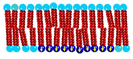
Figure 1: An asymmetric bilayer with a domain with a dipole density.

The phase diagram of lipid mixtures is a result of the microscopic characteristics of the lipids involved such as hydrocarbon chain and length as well as degree of saturation, possibility of forming hydrogen bonds, etc.. It is expected that the effect of these interactions is parameterized on longer scales by quantities such as a line tension $\gamma$ between coexisting domains, a spontaneous curvature $c_{0}$ of the different phospholipid species, the membrane surface tension $\tau$ or its bending rigidity $\kappa$ (see for example Gozdz2001 ; Harden2005 and references therein). The incorporation of the microscopic permanent dipoles of the lipids in these long wavelength descriptions is subtle. As an example, let us consider a bilayer containing a circular domain with non-zero dipolar density within a matrix of an hypothetical dipole free lipid, as shown in Fig. 1. The electrostatic free energy cost of such domain can be estimated in analogy with the monolayer case Keller1987 ; McConnell1988

$$F\approx R(a+b\log R)\ ,$$ (1)

where $R$ is the size of the domain. If the coefficient $b$ were vanishingly small, the net electrostatic cost of the dipoles grows with the perimeter of the domain and may be lumped into a “renormalized” line tension contribution. For the case shown in Fig. 1, however, the coefficient $b$ is not negligible, and the free energy contribution of the permanent dipoles must be considered explicitly. In some other situations, however, the coefficient $b$ may vanish. It seems plausible that if the domain in Fig. 1 was opposed by an identical domain of the same lipid, the membrane would not exhibit a permanent dipole moment and the electrostatic contribution would consist of a short-ranged interaction that might be incorporated into the line tension. Furthermore, ionic strength, by weakening the electrostatic interactions, can also influence domain sizes. In this paper we present a detailed quantitative analysis for these questions.

In all previous treatments of dipolar domains (such as McConnell1988 and all subsequent work), the free energy has been computed by directly summing over dipoles. In this paper, we will consider two oppositely charged sheets and obtain the free energy of the dipoles as the first non-trivial coefficient in the limit of small sheet separation. Obtaining the dipolar result in this way is particularly convenient for implementing the boundary conditions that should be met by dipole densities within layers with different dielectric constants.

The organization of the paper is as follows. In Sect. II we derive an explicit form for the free energy of the system. A summary of the exact solution for the electrostatic free energy of dipolar domains is provided in Sect. III. The details of the solution are mathematically dense so we defer the complete derivation to appendix A. In Sect. IV we analyze the theoretical implications for monolayers and bilayers domains. We conclude our paper with a discussion on some of the consequences of our results in Sect. V.

II Electrostatic Free Energy

We consider a system of three slabs with different dielectric constants and Debye lengths. Two disks of opposite surface charges parallel to each other are located on the boundaries of the middle slab, as shown in Fig. 2. The distance $D$ between the two oppositely charged disks is assumed smaller than any other length in the problem and therefore the two disks represent a dipolar density. In the dilute electrolyte regime, the free energy of the system consists of an ideal and an electrostatic term, Safran1994

$$F = k_{B}T\sum_{a}\int d^{3}{\bf r}n_{a}({\bf r})(\log(vn_{a}({\bf r}))-1)+$$ (2)

$$+ \frac{1}{8\pi}\int d^{3}{\bf r}\vec{E}\cdot\vec{D}\ ,$$

where $n_{a}({\bf r})=n_{a}^{B}\exp(-\frac{q_{a}e\Phi({\bf r})}{k_{B}T})$ is the number density of ions of type $a$, ionic valence $q_{a}$ and bulk concentration $n_{a}^{B}$. It is convenient to express the free energy in a different form. For the ideal part we write

$$\sum_{a}\int d^{3}{\bf r}n_{a}({\bf r})(\log(vn_{a}({\bf r}))-1)$$ (3)

$$= -\sum_{a}\frac{q_{a}e}{k_{B}T}\int d^{3}{\bf r}n_{a}({\bf r})\Phi({\bf r})+\sum_{a}N_{a}(\log(n_{a}^{B}v)-1)$$

$$= -\sum_{a}\frac{q_{a}e}{k_{B}T}\int d^{3}{\bf r}n_{a}({\bf r})\Phi({\bf r})+\sum_{a}N_{a}(\log(v\frac{N_{a}}{V})-1)-$$

$$- \sum_{a}n_{a}^{B}\int d^{3}{\bf r}(\exp(-\frac{q_{a}e\Phi({\bf r})}{k_{B}T})-1)\ ,$$

where the last term follows from the identity $N_{a}=\int d^{3}{\bf r}n_{a}^{B}\exp(-\frac{q_{a}e\Phi({\bf r})}{k_{B}T})$, where $N_{a}$ is the number of ions of type $a$ within the solution. The electrostatic term is written as

$$\frac{1}{8\pi}\int d^{3}{\bf r}\vec{E}\cdot\vec{D}=-\frac{1}{8\pi}\int d^{3}{\bf r}\nabla\Phi({\bf r})\cdot\vec{D}$$

$$= \frac{1}{2}\int d^{3}{\bf r}e\Phi({\bf r})\sum_{a}q_{a}n_{a}({\bf r})+\frac{1}{2}\int d^{3}{\bf r}e\Phi({\bf r})\sigma({\bf r})$$

The previous expressions are general for an interface in contact with a dilute ionic solution. Dipolar interactions are weak so we further assume the “Debye-Huckel” approximation $\frac{e\Phi({\bf r})}{k_{B}T}<<1$. The ion number density becomes

$$n_{a}({\bf r})=n_{a}^{B}(1-q_{a}\frac{e\Phi({\bf r})}{k_{B}T}+\frac{1}{2}\frac{q_{a}^{2}e^{2}(\Phi({\bf r}))^{2}}{(k_{B}T)^{2}}+..).$$ (5)

Upon using the charge neutrality condition $\sum_{a}q_{a}n_{a}^{B}=0$, it follows

$$\sum_{a}q_{a}n_{a}({\bf r}) = -(\sum_{a}q_{a}^{2}n_{a}^{B})\frac{e\Phi({\bf r})}{k_{B}T}+\cdots$$ (6)

$$\sum_{a}q_{a}\int d^{3}{\bf r}n_{a}({\bf r})\frac{e\Phi({\bf r})}{k_{B}T} = -\sum_{a}q_{a}^{2}n_{a}^{B}\int d^{3}{\bf r}(\frac{e\Phi({\bf r})}{k_{B}T})^{2}.$$

Inserting Eq. 3, Eq. II, Eq. 5 and Eq. 6 into Eq. 2 the free energy is

$$F=\frac{1}{2}\int d^{3}{\bf r}\Phi({\bf r})\sigma({\bf r})+k_{B}T\sum_{a}N_{a}(\ln(\frac{N_{a}}{V}v)-1).$$ (7)

The first term is the electrostatic free energy of the charged disks. It is remarkable that both the entropic and the electrostatic terms involving the ions explicitly cancel out. The second term is the ideal free energy of the ion species in solution. The subsequent analysis will be performed within the canonical ensemble where the total number of particles of the different species is fixed, so the ideal free energy is constant and will be ignored herein. For uniformly charged interfaces, the free energy can be further simplified to

$$F=\pi|\sigma|\int_{0}^{\infty}d\rho\rho(\Phi(\rho,-\frac{D}{2})-\Phi(\rho,\frac{D}{2})).$$ (8)

A complete evaluation of the free energy requires the determination of the electric potential, which follows from the Poisson-Boltzmann (PB) equation

$$\nabla^{2}\Phi({\bf r})=\frac{1}{\lambda_{D}^{2}}\Phi({\bf r})$$ (9)

where $\lambda_{D}$ is the Debye length. In regions where no ions are present ($\lambda_{D}=\infty$) and the previous equation reduces to the standard Poisson equation. In this paper, we consider problems with cylindrical symmetry. The solution to the PB equation is

$$\Phi(\rho,z)=a(k)\exp(\pm kz)J_{0}(\rho(k^{2}-1/\lambda_{D}^{2})^{1/2})\ ,$$ (10)

where $J_{0}(x)$ is the 0th order Bessel function and $k$ indexes different solutions.

The electric potential is

$$\Phi(\rho,z)=\left\{\begin{array}[]{l c}\int^{\infty}_{0}dkJ_{0}(k\rho)\frac{\exp(-(k^{2}+1/(\lambda_{D}^{a})^{2})^{1/2}z)}{(k^{2}+1/(\lambda_{D}^{a})^{2})^{1/2}}a_{1}(k)&z>D/2\\ \int^{\infty}_{0}dkJ_{0}(k\rho)(\frac{\exp((k^{2}+1/(\lambda_{D}^{b})^{2})^{1/2}z)}{(k^{2}+1/(\lambda_{D}^{b})^{2})^{1/2}}a_{2}(k)+\frac{\exp(-(k^{2}+1/(\lambda_{D}^{b})^{2})^{1/2}z)}{(k^{2}+1/(\lambda_{D}^{b})^{2})^{1/2}}a_{3}(k))&-D/2<z<D/2\\ \int^{\infty}_{0}dkJ_{0}(k\rho)\frac{\exp((k^{2}+1/(\lambda_{D}^{c})^{2})^{1/2}z)}{(k^{2}+1/(\lambda_{D}^{c})^{2})^{1/2}}a_{4}(k)&z<-D/2\end{array}\right.\ ,$$ (11)

The condition that the electric field must vanish at infinity ($E_{z}(\infty)=E_{z}(-\infty)=0$) has been already implemented. The values of $\lambda_{D}^{a,b,c}$ are the Debye lengths in each region. We further assume a different dielectric constant $\varepsilon^{a,b,c}$ for each region.

The coefficients $\{a_{i}(k)\}_{i=1\cdots 4}$ are determined from the boundary conditions

$$\Phi(\rho,(D/2)^{+}) = \Phi(\rho,(D/2)^{-})$$

$$\Phi(\rho,(-D/2)^{+}) = \Phi(\rho,(-D/2)^{-})$$

$$\varepsilon_{a}E_{z}(\rho,(D/2)^{+})-\varepsilon_{b}E_{z}(\rho,(D/2)^{-}) = -4\pi|\sigma|\Theta(R-\rho)$$

$$\varepsilon_{b}E_{z}(\rho,(-D/2)^{+})-\varepsilon_{c}E_{z}(\rho,(-D/2)^{-}) = 4\pi|\sigma|\Theta(R-\rho)$$ (12)

$$\ ,$$

where $E_{z}$ is the component of the electric field along the z-axis, which is assumed to be perpendicular to the plane defined by the disks. The boundary conditions defined by Eq. II are easily implemented by recalling the following identity for Bessel functions

$$\Theta(R-\rho)=\int^{\infty}_{0}dkJ_{0}(k\rho)J_{1}(kR)\ ,$$ (13)

where $\Theta(x)$ is Heaviside-$\Theta$ function defined by $\Theta(x)=1$ if $x>0$ and $\Theta(x)=0$ for $x<0$.

For further reference, we quote the free energy of two infinite disks of uniform and opposite charges filled with a medium of dielectric constant $\varepsilon_{I}$. The free energy of this system is equivalent to the elementary formula of an infinite capacitor

$$F_{C}=\frac{2\pi^{2}}{\varepsilon_{I}}|\sigma|^{2}R^{2}D.$$ (14)

We also will need the non-ideal free energy for the Guoy-Chapman diffuse layer of a weakly charged system $\lambda_{D}/\lambda_{G}<<1$, where $\lambda_{D}$ is the Debye length and $\lambda_{G}$ is the Guoy-Chapman length. The free energy is given by

$$F_{GC}=\frac{2\pi^{2}}{\varepsilon_{w}}|\sigma|^{2}R^{2}\lambda_{D}.$$ (15)

We note that upon replacing $\varepsilon_{I}$ by the dielectric constant of the solvent $\varepsilon_{w}$ and the finite size $D$ by the Debye length $\lambda_{D}$, the “capacitor”formula Eq. 14 is identical with the previous equation. With the explicit form of the potential Eq. 11 introduced into Eq. 7, the free energy of the system is

$$F=\frac{2\pi^{2}}{\varepsilon_{I}}|\sigma|^{2}R^{2}D{\cal F^{I}}(\frac{D}{R},\frac{R}{\lambda_{D}})\ ,$$ (16)

where ${\cal F^{I}}(x,y)$ is a function specific for each situation, which according to Eq. 14 satisfies ${\cal F^{I}}(0,0)=1$. In the following we provide an explicit calculation for the function ${\cal F^{I}}(x,y)$ in different cases.

III Exact results for the free energy in several cases

We provide an explicit solution for the following three problems shown in Fig. 2. In all cases, two infinitely thin disks of finite radius $R$ and uniform but opposite charges are separated by a distance $D$, and it is assumed that $R>>D$. In Problem A) the two disks are on the boundary of a medium of dielectric constant $\varepsilon_{I}$, with only one domain in contact with a salty solution with solvent of dielectric constant $\varepsilon_{w}$ (water) and the other domain in contact with a medium of dielectric $\varepsilon_{A}$. In problem B) both domains are in contact with a salty solution with solvent of dielectric $\varepsilon_{w}$, while the interior contains a polarizable medium of dielectric constant $\varepsilon_{I}$. In Problem C) the two domains are submerged in a solution with solvent of dielectric $\varepsilon_{w}$.

The free energy of these three systems can be computed exactly. The most relevant results are summarized below. Explicit formulas and complete details of the derivation are provided in appendix A.

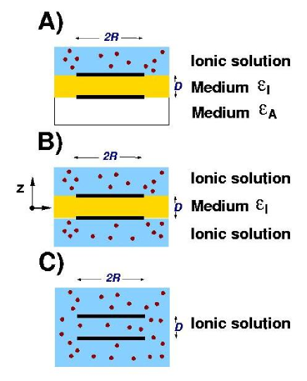
Figure 2: Two domains of uniform and opposite charges in contact with: A) one side with a salty solution, a medium in between and a different medium in the outside. B) Both sides in contact with a salty solution and a medium in between. C) submerged in a salty solution.

III.1 Finite circular dipole domain in a medium of dielectric $\varepsilon_{I}$ with one side in contact with a salty solution and the other with a medium of dielectric $\varepsilon_{A}$

The free energy for this system is given by the general expression

$$F^{A} = \frac{2\pi^{2}}{\varepsilon_{I}}|\sigma|^{2}R^{2}D\left(1-\right.$$

$$- \frac{D}{\pi R}\left.\{f_{1}(\frac{R}{\lambda_{D}})\ln(R/D)+f_{2}(\frac{R}{\lambda_{D}})\}\right)$$

where $f_{1}(y)$ and $f_{2}(y)$ are analytic functions of $y$. In the limit $y\rightarrow 0$ ($R/\lambda_{D}<<1$, low screening limit) and $y\rightarrow\infty$ ($R/\lambda_{D}>>1$, high screening limit) both $f_{1}$ and $f_{2}$ can be computed analytically. The results for $f_{1}$ are

$$f_{1}(0) = 2\frac{\varepsilon_{w}\varepsilon_{A}}{\varepsilon_{I}(\varepsilon_{w}+\varepsilon_{A})}$$

$$f_{1}(\infty) = 2\frac{\varepsilon_{A}}{\varepsilon_{I}}$$ (18)

Explicit formulas for $f_{2}$ and further details of the calculation are provided in appendix A.1.

III.2 Finite circular dipole domain within a medium of dielectric $\varepsilon_{I}$ both sides in contact with an aqueous solution

The free energy adopts different forms. In the low screening limit it reduces to a similar expression as in the previous case,

$$F^{B}=\frac{2\pi^{2}}{\varepsilon_{I}}|\sigma|^{2}R^{2}[1-\frac{D}{\pi R}(f_{1}\ln(R/D)+f_{2})]$$ (19)

where $f_{1}=\frac{\varepsilon_{w}}{\varepsilon_{I}}$ and the explicit expression for $f_{2}$ is quoted in Eq. 45.

In the high screening limit, there are two situations that need to be considered, $R>>\lambda_{D}>>D$ and $R>>D>>\lambda_{D}$. For $R>>\lambda_{D}>>D$ it is found

$$F^{B}=2\frac{2\pi^{2}}{\varepsilon_{I}}|\sigma|^{2}R^{2}D(1+{\cal O}(D/\lambda_{D})).$$ (20)

This result is derived for a simplified problem discussed below. In the limit $R>>\lambda_{D}>>D$ it follows

$$F^{B}=2\frac{2\pi^{2}}{\varepsilon_{w}}|\sigma|^{2}R^{2}\lambda_{D}.$$ (21)

Explicit formulas and detailed calculations are provided in appendix A.2.

III.3 Two oppositely charged disks in solution

The low screening limit has the same form as in Problem A. In the high screening limit, and for $D>>\lambda_{D}$, the system consists of two infinitely thin disks with diffuse layers on both sides interacting through a screened Coulomb potential,

$$F^{C}=\frac{2\pi^{2}}{\varepsilon_{w}}|\sigma|^{2}R^{2}\lambda_{D}(1-\exp{(-D/\lambda_{D})}).$$ (22)

In the high screening limit, but for $R>>\lambda_{D}>>D$, the leading term of the free energy is the “capacitor” term and is given by

$$F^{C}=\frac{2\pi^{2}}{\varepsilon_{I}}|\sigma|^{2}R^{2}D(1-\frac{D}{2\lambda_{D}})\ .$$ (23)

The first correction is independent of the radius $R$ of the domain. The details of the calculation are provided in appendix A.3.

IV Implications for monolayers and lipid domains

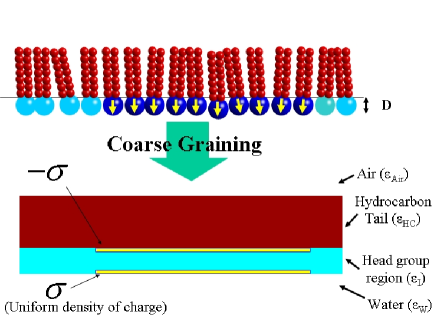
Figure 3: A Langmuir monolayer with a domain with a finite dipole density. The monolayer head group is represented as a medium with dielectric constant $\varepsilon_{I}$ within two opposite charge planes with uniform surface charges, one side in contact with an aqueous solution and the other with a medium of dielectric constant $\varepsilon_{HC}$ (the hydrocarbon tail).

IV.1 Monolayers

We consider a monolayer with dielectric constant $\varepsilon_{I}$ in between water $\varepsilon_{w}\approx 80$ and air $\varepsilon_{Air}\approx 1$. The monolayer consists of a minority phase of $n_{s}$ domains with radius $R$ and dipolar density $\mu\equiv\sigma D$ contained within a matrix of a majority phase with zero dipolar density, as shown in Fig. 3. The area spanned by the minority phase is $A_{s}\equiv n_{s}\pi R^{2}$. The free energy is constructed from the coarse-graining suggested in Fig. 3, which consists of approximating the head group region as a medium of dielectric constant $\varepsilon_{I}$ and the hydrocarbon tail as an infinite medium of dielectric constant $\varepsilon_{HC}$. From the results in Subsect. III.1 it is

$$F_{tot}=(2\pi\gamma R+F^{A})\frac{A_{s}}{\pi R^{2}},$$ (24)

where $\gamma$ is the line tension between the two phases. The free energy explicitly depends on the domain radius $R$, and is minimized under the constraints of both constant dipolar density $\mu$ and minority phase area $A_{s}$. The equilibrium radius of the domains $R_{eq}$ is given from

$$R_{eq}=D\exp(1-\frac{f_{2}}{f_{1}})\exp(\frac{\varepsilon_{I}\gamma}{f_{1}\mu^{2}})\approx D\exp(\frac{\varepsilon_{I}\gamma}{f_{1}\mu^{2}}).$$ (25)

The above expression is only exact in the limits $y\rightarrow 0$ (low screening) and $y\rightarrow\infty$ (high screening), as otherwise terms involving derivatives of $f(y)$ are present. From Eq. III.1, as a result of $\varepsilon_{w}>>\varepsilon_{A}=\varepsilon_{HC}$, it is found $f_{1}(0)\approx f_{1}(\infty)$. It also follows from Eq. A.1.1 that $f_{2}(0)\approx f_{2}(\infty)$. Therefore, for both the low and high screening limits, the domain radius is the same and is given by

$$R_{eq}\approx D\exp(\frac{\varepsilon_{I}^{2}\gamma}{2\varepsilon_{HC}\mu^{2}}).$$ (26)

The term in the exponent is only half of the value originally obtained by McConnell Keller1987 ; McConnell1988 and it is multiplied by the factor $\varepsilon_{I}^{2}/\varepsilon_{HC}$. For the case $\varepsilon=1$, it agrees, upto the 1/2 factor, with the result for stripes obtained in Andelman1987 . The origin of the $1/2$ factor is the discontinuity in the dielectric constant between air and water, while the presence of the different dielectric constants is due to the finite polarizability of the dipoles and the surrounding medium.

The same formula applies for a more general situation where the matrix has a non-zero dipole density $\mu_{1}$ and the domains a dipolar density $\mu_{2}$. In that case, the quantity appearing in the exponent is the dipolar density difference $\mu=|\mu_{2}-\mu_{1}|$.

IV.2 Bilayers

We now consider a bilayer with a circular domain, where the dipolar density of the outer leaflet ($\mu_{1}$) and the inner leaflet ($\mu_{2}$) are different. Similarly as in the case for monolayers, the dipolar densities are to be interpreted as the excess dipolar density from the matrix reference state. The domain has radius $R$ and the vertical separation between the two leaflets is $L$, as shown in fig. 4. The bilayer is surrounded by water ($\varepsilon_{w}\approx 80$). As shown in appendix B, the electrostatic free energy cost is of the form

$$F_{ele}\sim-(\mu_{1}-\mu_{2})^{2}R\ln(\frac{8R}{L})+\gamma^{\prime}2\pi R,$$ (27)

where terms proportional to $R^{2}$ have been ignored as they are not relevant for this argument. For a symmetric domain ($\mu_{1}=\mu_{2}$) there is no logarithmic contribution and the electrostatic free energy is of the same form as the line tension. The above result has been derived without including the effects of ionic strength or different dielectric constants, but we assume it true under these more general conditions.

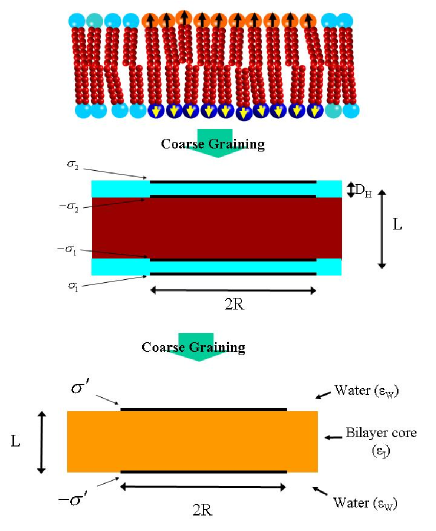
Figure 4: Dipolar domains in a bilayer. In a first approximation, the two leaflets of the bilayer are modelled as two monolayers, an inner leaflet monolayer with dipolar density $\mu_{2}\equiv\sigma_{2}D$ and an outer leaflet monolayer with $\mu_{1}\equiv\sigma_{1}D$, following the same steps as in Fig. 3. At longer distances, the net dipolar moment of the two monolayers can be represented as if were originated by two oppositely charged disks with charge density $\sigma^{\prime}=(\sigma_{1}-\sigma_{2})D/L$, with an effective dielectric constant $\varepsilon_{I}$ taking into account both hydrocarbon tail and head groups polarizabilities.

If the membrane contains an intrinsic asymmetry between the inner and outer leaflets (for definiteness, we assume $\mu_{1}\ >\mu_{2}$), there is a net dipolar moment. We consider domains much larger than the vertical separation of the two leaflets ($R>>L$), and construct the free energy by first coarse-graining each separate leaflet of the bilayer following the same steps as in the monolayer case. The bilayer has a net dipolar moment, which we model as if it were produced by two disks of uniform but opposite surface charge density $\sigma^{\prime}$, where $\sigma^{\prime}=(\sigma_{1}-\sigma_{2})D_{H}/L$ and $D_{H}$ is the width of the head group region. This argument should not be understood as implying that the coarse-graining of an asymmetric bilayer should lead to equal and opposite charge distributions, but rather that this configuration leads to the same dipolar moment. It is expected that higher order moments provide sub-leading corrections, which nevertheless may be incorporated as any other short-range interactions, if necessary. The dielectric constant $\varepsilon_{I}$ is an effective value that includes contributions both from the hydrocarbon tails and the head group and therefore it should be expected that $\varepsilon_{I}\sim 4$. The different steps in the coarse graining process are illustrated in Fig. 4. Under these assumptions, the problem of an asymmetric domain is reduced to the problem discussed in Subsect. III.2. In the low screening limit, the radius of $n_{s}$ domains is computed as for the monolayer case, and is given by

$$R_{eq}\approx L\exp(\frac{\varepsilon_{I}^{2}\gamma}{\varepsilon_{W}(\mu_{1}-\mu_{2})^{2}})\ ,$$ (28)

where $\varepsilon_{I}$ is the effective dielectric constant including contributions from the hydrocarbons and the polarizabilities of the dipoles. This formula differs from the analogous result for monolayers in the factor $\varepsilon_{w}/2\varepsilon_{HC}\approx 10$ in the exponent, which implies that if a given dipole density and line tension in a monolayer leads to an equilibrium radius $R_{eq}\approx 10\mu M$, the same dipolar density and line tension in a bilayer results in much smaller domains, of radius comparable to the molecular scale (of the order of $L$). Alternatively, the previous formula shows that the condition for large (micron sized) domains to exist is given by

$$\frac{\varepsilon_{I}^{2}\gamma}{\varepsilon_{w}\mu^{2}}\approx 8\rightarrow\Delta p\approx\varepsilon_{I}A_{0}\sqrt{\frac{k_{B}T}{8\varepsilon_{w}L^{\prime}}}\ ,$$ (29)

where $p$ is the permanent moment of the phospholipid, $A_{0}$ is the molecular area and we assumed that the line tension is $\gamma\approx\frac{k_{B}T}{L^{\prime}}$. With $A_{0}\approx 60$ Ų, $L^{\prime}\approx 10$ Å, the formula yields $\Delta p<<0.1\varepsilon_{I}$ (D). If we assume $\varepsilon_{I}\approx 4$ then $\Delta p<<0.4$ D. That is, a net dipolar moment difference of the order of $0.4$ D or less is needed for large (micron sized) dipolar domains to be observed. Dipolar moments for phospholipids are much larger, of the order of $15$ D Gawrisch1992 , which implies that domains with significant asymmetry will be sub-micron in size.

In the high screening limit, the results are qualitatively different. When the Debye length becomes of the order of the domain radius, the electrostatic interactions become short-ranged and the free energy, which is given in Eq. 21, does not show the logarithmic contribution present in Eq. 27. In that case, the thermodynamic stable state of the $n_{s}$ domains is completely dominated by line tension and the free energy is minimized by a single circular domain (assuming that the resulting line tension is positive) of the minority phase within a matrix of the majority phase. A summary of the different results is shown in Fig. 5.

V Discussion and conclusions

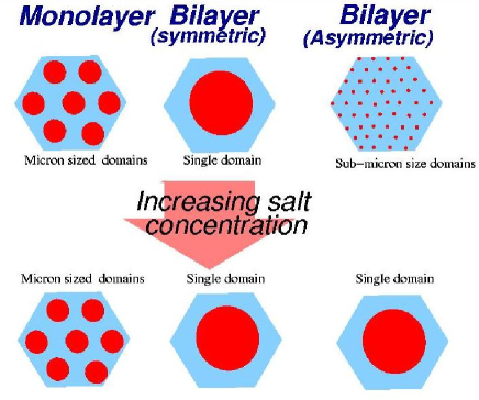
Figure 5: Schematic representation of the different systems studied upon variations in ionic strength.

We presented a detailed calculation showing how the competition between line tension and electrostatic dipolar interactions determines the size of lipid domains, thus extending previous results by McConnell and collaborators Keller1987 ; McConnell1988 by including finite ion strength, variations in the dielectric constant and the polarizability of the dipoles and further extending the results to account for dipolar domains in lipid membranes. The main conclusions are summarized in Fig. 5; for lipid monolayers at the air-water interface it is found that the size of the lipid domains is independent of the ionic strength, but is sensitive to the discontinuities in dielectric constant and the polarizability of the dipoles. In lipid vesicles, it has been shown that for symmetric domains, where the net dipole density in the outer and inner leaflet is the same, the electrostatic contribution to the free energy can be absorbed into the line tension coefficient. For asymmetric domains, which have a net dipolar density, it has been shown that the large dielectric constant of water is responsible for a dramatic decrease of the size of the domains as compared with the size obtained for a monolayers with the same line tension and dipole density. It has also been shown that small variations in dipolar density (2$\%$ or more from the equilibrium dipole density of a zwitterionic phospholipid) are enough to limit domain sizes to sub-micron scales. Opposite to the situation with monolayers, dipolar domains in bilayers are sensitive to solution ionic strength. At small Debye lengths, of the order of the domain radius at zero ionic strength, dipolar electrostatic effects gradually become negligible and the system is dominated by line tension, resulting in a single large circular minority domain if the line tension is positive. Our study has been focused on the limiting cases of high and low ionic strength, but exact analytic expressions have been provided for the free energy and the electric potential. Problems that have not been discussed in this paper, such as values for domain radius at intermediate ionic strength, ionic distributions or potential differences across the interface also follow from these expressions.

Our results show the subtle role played by the intrinsic dipoles in lipids membranes. At high ionic strength, the effect of dipoles is short-ranged, but at low ionic strength dipolar interactions are only negligible for symmetric domains, and in any other situation, dipolar interactions must be included explicitly, either in continuum models Gozdz2001 ; Harden2005 or in numerical simulations Stevens2004 .

Recent experimental and theoretical studies have studied the interactions of circular and planar dipolar domains Khattari2002 and interactions within two domains Wurlitzer2002 . As compared with previous theoretical studies Smorodin2001 of domain shape transitions in lipid bilayers, our study includes the effects of a net dipolar moment and the dielectric constant of water. More importantly, it shows that at high ionic strength the effect of dipolar interactions is short-ranged. Other theoretical work Netz1999 has discussed interfaces within the framework of the Debye-Huckel approximation, the same approximation used in this study, but has been focused on effective interactions between charges, so these results are somewhat complementary to the ones presented here.

A number of situations have not been considered in this paper. Our study has been restricted to circular domains, while other shapes, such as stripes, are also of interest Keller1987 ; Seul1995 . We further assumed a planar membrane, thus neglecting the effects of Gaussian curvature, which has been shown that, at least for solid domains, may lead to significant effects Travesset2005 ; Travesset2006 ; Bowick2006 . The results presented have ignored domain-domain interaction and its possible superstructures. This problem is discussed in Seul1995 , where it is shown that triangular lattices of circular domains are usually found, and a discussion is presented on the transition from circular to other domains and other phases such as stripes Keller1999 .

Problems where dipolar-like domains, similar to the ones considered in this paper, have been discussed in other contexts. The free energy describing the phase transition between a Fermi liquid and an insulating Wigner crystal phase in a clean two dimensional electron can be mapped to a dipolar interaction and a line tension term. After a detailed analysis, the authors in Spivak2003 showed that a direct first order phase transition cannot occur, and instead, it was shown that the transition should proceed as a sequence of intermediate “microemulsion”phases, consisting of domains of one phase within a matrix of the other phase. Our results are in complete agreement with Spivak2003 , but show that a direct first order transition can be obtained as a function of the Debye length, if the electrostatic interactions are screened. Previous MD simulations Reichhardt2003a ; Reichhardt2003b have shown that transitions from triangular superlattices to striped domains are a general feature resulting from increasing the strength of a short-ranged attraction force with respect to a long range repulsion. Upon identifying the short-range attraction with the line tension and the long range repulsion with the dipolar interactions, these results are qualitatively similar to the problems studied in this paper. It seems therefore that “microemulsion”phases are a common feature of systems near a phase transition consisting of a long range repulsion and short a range attraction. In fact, this has been shown rigorously for general 2D Coulomb systems Jamei2005 . Another interesting example is provided by heteroepitaxial growth of 2D islands in solid surfaces, where the elastic free energy cost of assembling an island also contains a logarithmic term (completely analogous with the dipolar case studied in this paper) and competes against the line tension. In Liu2001 , it was shown that the addition of domain-domain interactions in the form of dipolar interactions leads to the formation of triangular superlattices. These results show that interactions among finite circular domains are responsible for the formation of superlattice structures of circular domains, whose size can be computed from balancing elastic (or dipolar) free energy against line tension, and provide yet another example illustrating the expected general results of phase separations in systems with long range interactions.

It is quite interesting to compare the exact solutions discussed in Sect. III with the corrections to a finite size capacitor, as discussed Landau  &  Lifshitz Landau2004 . Although the charge distribution in the plates of a finite size capacitor is not uniform, as we assume in our calculations, the coefficient of the logarithmic term $f_{1}$ in the electrostatic energy for $\varepsilon_{I}=\varepsilon_{A}=\varepsilon_{W}$, Eq. A.1.1 is identical with the analogous formula quoted in Landau  &  Lifshitz Landau2004 .

This paper has shown the subtle role played by dipolar moments. We showed that the zwitterionic nature of the phospholipids leads to new effects both in bilayers and monolayers. It is our expectation that the results presented will be useful in other areas.

acknowledgements

I thank A. Grosberg and J. Israelachvili for proposing this problem and for many discussions. I also acknowledge discussions with C. Lorenz and D. Vaknin. I acknowledge the Benasque Center for Sciences, where this work was started. This work is supported by NSF grant DMR-0426597 and partially supported by DOE through the Ames lab under contract no. W-7405-Eng-82.

Appendix A Detailed derivation of the expressions for the free energy

A.1 Finite circular dipole domain in a medium of dielectric $\varepsilon_{I}$ with one side in contact with a salty solution and the other with a medium of dielectric $\varepsilon_{A}$

This situation corresponds to case A) in Fig. 2. There are three dielectric constants, the medium in between the disks ($\varepsilon^{b}=\varepsilon_{I}$), the medium outside the disks ($\varepsilon^{c}=\varepsilon_{A}$) and the dielectric of the solvent $\varepsilon^{a}=\varepsilon_{w}$ (water). The electric potential in the different region follows from Eq. 10 with both $\lambda_{D}^{b}=\lambda_{D}^{c}=\infty$.

The coefficients $\{a_{i}(k)\}_{i=1\cdot 4}$ are determined from the boundary conditions Eq. II with the help of Eq. 13. The explicit result for the $a_{4},a_{3}$ coefficients are

$$a_{1}(k) = \frac{-(\sinh(kD/2)+\frac{\varepsilon_{A}}{\varepsilon_{I}}\cosh(kD/2))\sinh(kD/2)\exp((k^{2}+1/\lambda_{D}^{2})^{1/2}D/2)}{\frac{\cosh(kD/2)}{\varepsilon_{I}}(\frac{\varepsilon_{w}}{k}+\frac{\varepsilon_{A}}{(k^{2}+1/\lambda_{D})^{1/2}})+\sinh(kD/2)(\frac{\varepsilon_{A}\varepsilon_{w}}{k\varepsilon_{I}^{2}}+\frac{1}{(k^{2}+1/\lambda_{D})^{1/2}})}\frac{8\pi|\sigma|R}{k\varepsilon_{I}}J_{1}(kR)$$

$$a_{4}(k) = \frac{(\frac{k\sinh(kD/2)}{(k^{2}+1/\lambda_{D}^{2})^{1/2}}+\frac{\varepsilon_{w}}{\varepsilon_{I}}\cosh(kD/2))\sinh(kD/2)\exp((k^{2}+1/\lambda_{D}^{2})^{1/2}D/2)}{\frac{\cosh(kD/2)}{\varepsilon_{I}}(\frac{\varepsilon_{w}}{k}+\frac{\varepsilon_{A}}{(k^{2}+1/\lambda_{D})^{1/2}})+\sinh(kD/2)(\frac{\varepsilon_{A}\varepsilon_{w}}{k\varepsilon_{I}^{2}}+\frac{1}{(k^{2}+1/\lambda_{D})^{1/2}})}\frac{8\pi|\sigma|R}{k\varepsilon_{I}}J_{1}(kR)$$

The explicit form for free energy follows from Eq. 8

$$F=\frac{2\pi^{2}}{\varepsilon_{I}}|\sigma|^{2}R^{2}D{\cal F^{A}}(\frac{D}{R},\frac{R}{\lambda_{D}})\ ,$$ (31)

where ${\cal F^{A}}(x,y)$ is given by

$${\cal F^{A}}(x,y)=4\int^{\infty}_{0}\frac{dk}{k^{2}}J^{2}_{1}(k)\frac{\sinh(kx/2)}{x}\frac{\cosh(kx/2)(\frac{a}{k}+\frac{b}{(k^{2}+y^{2})^{1/2}})+\sinh(kx)\frac{2}{(k^{2}+y^{2})^{1/2}}}{\cosh(kx/2)(\frac{a}{k}+\frac{b}{(k^{2}+y^{2})^{1/2}})+\sinh(kx)(\frac{ab}{k}+\frac{1}{(k^{2}+y^{2})^{1/2}})}\ .$$ (32)

In order to alleviate the notation, we have introduced new variables $a=\varepsilon_{w}/\varepsilon_{I}$ and $b=\varepsilon_{A}/\varepsilon_{I}$. In the strict $R>>D$ limit, the free energy corresponds to two infinite circular plates, as the function ${\cal F^{A}}$ satisfies

$$\lim_{x\rightarrow 0}{\cal F^{A}}(x,y)=1\ ,$$ (33)

irrespectively of the value for $y$. The first correction ${\cal O}(D/R)$ to the free energy is of the form

$$F = \frac{2\pi^{2}}{\varepsilon_{I}}|\sigma|^{2}R^{2}D(1-\frac{D}{\pi R}\{f_{1}(\frac{R}{\lambda_{D}})\ln(R/D)+f_{2}(\frac{R}{\lambda_{D}})\})$$ (34)

$$\ ,$$

where $f_{1}(y)$ and $f_{2}(y)$ are two analytic functions, whose limiting expressions in the low and high screening limits is provided below. The general derivation of the expression Eq. 34 follows from the same steps as the formula derived below for the restricted case of the low screening limit.

A.1.1 The low screening limit ($R<<\lambda_{D}$)

The function ${\cal F^{A}}$ must be considered in the limit $y\rightarrow 0$,

$${\cal F^{A}}(x,0) = \frac{4}{x}\int^{\infty}_{0}\frac{dk}{k^{2}}J^{2}_{1}(k)\sinh(kx/2)\frac{(a+b)\cosh(kx/2)+2\sinh(kx)}{(a+b)\cosh(kx)+(ab+1)\sinh(kx))}$$

$$= \frac{2}{x}\int^{\infty}_{0}\frac{dk}{k^{2}}J^{2}_{1}(k)(1-\exp{(-kx)})\frac{1+\frac{(2-a-b)}{2(a+b)}(1-\exp{(-kx)})}{1+\frac{(ab+1-a-b)}{2(a+b)}(1-\exp{(-2kx)})}.$$

This function is of the general form Eq. 62, where $A=\frac{2-a-b}{2(a+b)}$ and $B=\frac{ab+1-a-b}{2(a+b)}$. The general expression for the asymptotic behavior follows from the result in Eq. C,

$$f_{1}(0) = 2\frac{ab}{a+b}=2\frac{\varepsilon_{w}\varepsilon_{A}}{\varepsilon_{I}(\varepsilon_{w}+\varepsilon_{A})}$$

$$f_{2}(0) = 2\frac{ab}{a+b}\ln(8/(e^{1/2}))+\frac{(2-a-b)(2a+2b)}{(a+b)^{2}}-$$ (36)

$$- \frac{2(a+b)}{ab+1+a+b}\left({\cal G}_{1}(\frac{ab+1-a-b}{ab+1+a+b})-\right.$$

$$- \left.\frac{4-2a-2b}{a+b}{\cal G}_{2}(\frac{ab+1-a-b}{ab+1+a+b})\right)$$

where the functions ${\cal G}_{i}$ are defined in Eq. C. If both salt-free mediums have the same dielectric constant $\varepsilon_{I}=\varepsilon_{A}$, then $b=1$ and the expression for $f_{2}$ simplifies to

$$f_{2}(0)=\ln(8/e^{1/2})-\frac{1-a}{2(1+a)}\ln(4/e).$$ (37)

In Riviere1995 the coefficient $f_{1}(0)$ for a dipole domain with no polarization $\varepsilon_{I}=1$ was quoted, and the result is in agreement with Eq. A.1.1. McConnell and collaborators Keller1987 ; McConnell1988 have computed the free energy in the limit $\varepsilon_{w}=\varepsilon_{A}=\varepsilon_{I}=1$ by integrating the individual contributions of single dipoles and introducing a short-distance cut-off $\delta$ to avoid a self-energy singularity. Their result is

$$f_{1}(0) = 1$$ (38)

$$f_{2}(0) = \ln(e^{2}\delta/(4D))\ ,$$

which is identical with Eq. A.1.1 if the cut-off is taken as $\delta=D/(2e^{3/2})$.

A.1.2 The high screening limit $R>>\lambda_{D}$

We now consider the limit where the Debye screening is much shorter than the radius of the dipolar domain. We therefore need to consider the limiting case $y\rightarrow\infty$ in the scaling function Eq. 32. The resulting ${\cal F^{A}}$ is

$${\cal F^{A}}(x,\infty) = \frac{2}{x}\int^{\infty}_{0}\frac{dk}{k^{2}}J^{2}_{1}(k)(1-\exp{(-kx)})\frac{1-\frac{1}{2}(1-\exp{(-kx)})}{1+\frac{(b-1)}{2}(1-\exp{(-2kx)})}\ ,$$ (39)

which is of the general form Eq. 62, with $A=-1/2$ and $B=(b-1)/2$. The expressions for $f_{1}(\infty)$ and $f_{2}(\infty)$ coefficients follow as

$$f_{1}(\infty) = 2b=2\frac{\varepsilon_{A}}{\varepsilon_{I}}$$ (40)

$$f_{2}(\infty) = 2b\ln(8/e^{3/2})-\frac{2}{b+1}\left({\cal G}_{1}(\frac{b-1}{b+1})+\right.$$

$$+ \left.2{\cal G}_{2}(\frac{b-1}{b+1})\right)\ .$$

Both $f_{1}(\infty)$ and $f_{2}(\infty)$ are independent of $\varepsilon_{w}$. In the high screening limit, the electric field does not penetrate in the water, and therefore no reference to the dielectric properties of the water should be expected.

A.2 Finite circular dipole domain within a medium of dielectric $\varepsilon_{I}$ both sides in contact with an aqueous solution

This situation differs from the previous case in that the aqueous solution is in contact with both sides of the domain. The potential is screened everywhere except for the thin layer in between the two disks, where the dielectric constant is $\varepsilon_{I}$. The electric potential follows from Eq. 11, with $\lambda_{D}^{a}=\lambda_{D}^{c}=\lambda_{D}$ and $\lambda_{D}^{b}=\infty$.

Upon imposing the boundary conditions Eq. II the coefficients satisfy $a_{1}(k)=-a_{4}(k)$ and $a_{2}(k)=-a_{3}(k)$, with

$$a_{1}(k) = -(k^{2}+1/\lambda_{D}^{2})^{1/2}\exp{((k^{2}+1/\lambda_{D}^{2})^{1/2}D/2)}\frac{4\pi|\sigma|RJ_{1}(kR)\sinh(kD/2)}{(k^{2}+1/\lambda_{D}^{2})^{1/2}\varepsilon_{w}\sinh(kD/2)+k\varepsilon_{I}\cosh(kD/2)}$$

$$a_{2}(k) = -\frac{2\pi|\sigma|kRJ_{1}(kR)}{(k^{2}+1/\lambda_{D}^{2})^{1/2}\varepsilon_{w}\sinh(kD/2)+k\varepsilon_{I}\cosh(kD/2)}$$ (41)

and the free energy is

$$F=\frac{2\pi^{2}}{\varepsilon_{I}}|\sigma|^{2}R^{2}D{\cal F^{B}}(\frac{D}{R},\frac{R}{\lambda_{D}})\ ,$$ (42)

where ${\cal F^{B}}$ is defined from

$${\cal F^{B}}(x,y)=\frac{8}{x}\int^{\infty}_{0}dkJ^{2}_{1}(k)\frac{\sinh(kx/2)}{k(k^{2}+y^{2})^{1/2}}\frac{\cosh(kx/2)+\frac{\varepsilon_{I}k}{\varepsilon_{w}(k^{2}+y^{2})^{1/2}}\sinh(kx/2)}{(\frac{\varepsilon_{w}}{\varepsilon_{I}}+\frac{k^{2}}{(k^{2}+y^{2})})\sinh(kx)+\frac{2k}{(k^{2}+y^{2})^{1/2}}\cosh(kx)}\ .$$ (43)

In the low screening limit $R<<\lambda_{D}$, this function becomes of the general form Eq. 62 with $A=\frac{1}{2}(\frac{\varepsilon_{I}}{\varepsilon_{w}}-1)$ and $B=\frac{1}{4}(\frac{\varepsilon_{I}}{\varepsilon_{w}}+\frac{\varepsilon_{I}}{\varepsilon_{w}}-2)$, thus the free energy becomes

$$F=\frac{2\pi^{2}}{\varepsilon_{I}}|\sigma|^{2}R^{2}(1-\frac{D}{\pi R}\left\{f_{1}\ln(R/D)+f_{2}\right\})\ ,$$ (44)

where the coefficients are given from

$$f_{1} = \frac{\varepsilon_{w}}{\varepsilon_{I}}$$ (45)

$$f_{2} = \frac{\varepsilon_{w}}{\varepsilon_{I}}\ln(8/e^{1/2})+(\frac{\varepsilon_{I}}{\varepsilon_{w}}-1)(\frac{\varepsilon_{I}}{\varepsilon_{w}}+\frac{\varepsilon_{w}}{\varepsilon_{I}})-$$

$$- \frac{4}{2+\frac{\varepsilon_{I}}{\varepsilon_{w}}+\frac{\varepsilon_{w}}{\varepsilon_{I}}}\left({\cal G}_{1}(\frac{\frac{\varepsilon_{I}}{\varepsilon_{w}}+\frac{\varepsilon_{w}}{\varepsilon_{I}}-2}{\frac{\varepsilon_{I}}{\varepsilon_{w}}+\frac{\varepsilon_{w}}{\varepsilon_{I}}+2})-\right.$$

$$- \left.2(\frac{\varepsilon_{I}}{\varepsilon_{w}}-1){\cal G}_{2}(\frac{\frac{\varepsilon_{I}}{\varepsilon_{w}}+\frac{\varepsilon_{w}}{\varepsilon_{I}}-2}{\frac{\varepsilon_{I}}{\varepsilon_{w}}+\frac{\varepsilon_{w}}{\varepsilon_{I}}+2})\right)$$

These expressions are actually identical with Eq. A.1.1 with $a=b=\frac{\varepsilon_{w}}{\varepsilon_{I}}$.

The high screening limit ($\lambda_{D}<<R$) corresponds to $y\rightarrow\infty$. In this limit, ${\cal F}^{B}$ takes a particularly simple form

$${\cal F}^{B}(x,\infty)=\frac{4}{xy}\int^{\infty}_{0}dk\frac{J^{2}_{1}(k)\varepsilon_{I}}{k\varepsilon_{w}}=\frac{2\varepsilon_{I}}{xy\varepsilon_{w}}\ ,$$ (46)

leading to the free energy

$$F=2\frac{2\pi^{2}}{\varepsilon_{w}}|\sigma|^{2}R^{2}\lambda_{D}.$$ (47)

This result is significantly different from the low screening limit, as the free energy is independent of the separation between the two disks $D$, which has been replaced by the Debye length and the dielectric constant is no longer the dielectric constant of the membrane but that of the water. This expression is twice the free energy of the diffuse layer Eq. 15, and implies that the system minimizes the free energy by effectively decoupling the two charged disks into two diffuse layers, resulting in a zero electric field within the bilayer. This result also follows from noticing that the “Guoy-Chapman” free energy Eq. 47 is lower that the “capacitor” formula Eq. 14 whenever

$$\frac{D}{\varepsilon_{I}}>\frac{2\lambda_{D}}{\varepsilon_{w}}\ ,$$ (48)

which is always satisfied for a sufficiently small $\lambda_{D}$. There is another regime defined by $R>>\lambda_{D}$ and $\lambda_{D}>>D$ where the “capacitor” formula is still the leading term, but its corrections are ${\cal O}(D/\lambda_{D})$. This regime is discussed in detail in the next problem.

A.3 Two oppositely charged disks in solution

This situation is similar to the previous case, except that now both the solvent and the ions can be found in between the two plates. The electric potential follows from Eq. 11 with $\lambda_{D}^{a}=\lambda_{D}^{b}=\lambda_{D}^{c}$. The boundary conditions are given by the usual Eq. II, but only one dielectric constant appears ($\varepsilon_{I}=\varepsilon_{A}=\varepsilon_{w}$). The $a_{i}(k)$ coefficients satisfy $a_{3}(k)=-a_{2}(k)$ and $a_{1}(k)=-a_{4}(k)$, with

$$a_{1}(k) = -\frac{4\pi}{\varepsilon_{w}}|\sigma|RJ_{1}(kR)\sinh((k^{2}+1/\lambda_{D}^{2})^{1/2}D/2)$$

$$a_{2}(k) = -\frac{2\pi}{\varepsilon_{w}}|\sigma|RJ_{1}(kR)\exp(-(k^{2}+1/\lambda_{D}^{2})^{1/2}D/2)$$

The free energy is

$$F=\frac{2\pi^{2}}{\varepsilon_{w}}|\sigma|^{2}R^{2}D{\cal F^{C}}(\frac{D}{R},\frac{R}{\lambda_{D}})\ ,$$ (50)

where ${\cal F^{C}}$ is defined by

$${\cal F^{C}}(x,y)=\frac{2}{x}\int^{\infty}_{0}dkJ^{2}_{1}(k)\frac{1-\exp{(-(k^{2}+y^{2})^{1/2}x})}{k(k^{2}+y^{2})^{1/2}}$$ (51)

The low screening limit defined by $\lambda_{D}>>R$ ($y\rightarrow 0$) has already been considered as it is identical as the one considered in Sect. A.1 ( ${\cal F^{C}}(x,0)={\cal F^{A}}(x,0)$), whose limit is provided by Eq. A.1.1.

In the high screening limit ($R>>\lambda_{D}$), we consider two situations corresponding to either $D>>\lambda_{D}$ or $D<<\lambda_{D}$. In both cases the ${\cal F^{C}}$ function Eq. 51 needs to be evaluated for $y>>1$, but with the additional assumptions that either $xy>>1$ or $xy<<1$. For $xy>>1$ it is readily obtained

$${\cal F^{C}}(x,y)=\frac{1}{xy}(1-\exp{(-xy)})\ .$$ (52)

and the resulting free energy is

$$F=\frac{2\pi^{2}}{\varepsilon_{w}}|\sigma|^{2}R^{2}\lambda_{D}(1-\exp{(-D/\lambda_{D})})$$ (53)

The first term is the diffuse layer free energy of two finite, infinitely thin disks surrounded by a diffuse layer of counterions on both sides. In this case, each disk has a contribution that is exactly 1/2 of Eq. 15. The second term represents the Coulomb attraction of the two disk-charges, which is screened by the electrolytes.

The limit $xy<<1$ is more complex, and it is obtained from the following function

$${\cal Q_{J}}(x,y) = \int^{y}_{0}dkJ^{2}_{1}(k)\frac{1-\exp{(-(k^{2}+y^{2})^{1/2}x})}{k}$$ (54)

$$+ \int^{\infty}_{y}dkJ^{2}_{1}(k)\frac{1-\exp{(-(k^{2}+y^{2})^{1/2}x})}{k}$$

$$\ ,$$

which is related as $\frac{\partial{(x{\cal F^{C}}})}{{\partial x}}=2{\cal Q_{J}}$ (see Eq. 51). The first integral is expanded as

$$\int^{y}_{0}dkJ^{2}_{1}(k)\frac{1-\exp{(-(k^{2}+y^{2})^{1/2}x})}{k}$$

$$= \int^{y}_{0}\frac{dk}{k}J^{2}_{1}(k)-xy\int^{y}_{0}\frac{dk}{k}J^{2}_{1}(k)(1+k^{2}/y^{2})^{1/2}$$

$$= \int^{\infty}_{0}\frac{dk}{k}J^{2}_{1}(k)-\int^{\infty}_{y}\frac{dk}{k}J^{2}_{1}(k)+xy\int^{\infty}_{0}\frac{dk}{k}J^{2}_{1}(k)$$

$$= \frac{1-xy}{2}-\int^{\infty}_{y}\frac{dk}{k}J^{2}_{1}(k)+{\cal O}((xy)^{2}).$$

The second integral is computed from

$$\int^{\infty}_{y}dkJ^{2}_{1}(k)\frac{1-\exp{(-(k^{2}+y^{2})^{1/2}x})}{k}$$

$$= \frac{2}{\pi}\int^{y}_{0}\frac{dk}{k^{2}}(1-\sin(2k))\exp(-(k^{2}+y^{2})^{1/2}x)$$

$$= \frac{2}{\pi y}\int^{\infty}_{1}\frac{du}{u^{2}}(1-\sin(2yu))\exp(-xy(1+u^{2})^{1/2})$$

$$= \frac{2}{\pi y}(1+{\cal O}(xy))\ .$$

where the asymptotic expansion of the Bessel functions for large values of the argument have been used. Combining equations Eq. A.3 and Eq. A.3, and noticing that the terms of order $1/y$ cancel, it follows that

$${\cal Q_{J}}(x,y)=\frac{1-xy}{2}+{\cal O}((xy)^{2},(xy)/y)\ ,$$ (57)

which leads to the small x-expansion for ${\cal F^{C}}$,

$${\cal F^{C}}(x,y)=\frac{2}{x}(\frac{x}{2}-\frac{x^{2}y}{4}+\cdots)\ ,$$ (58)

or

$${\cal F^{C}}(x,y)=1-\frac{xy}{2}\ .$$ (59)

The free energy in the regime defined by $D<<\lambda_{D}$ and $R>>\lambda_{D}$ is therefore

$$F=\frac{2\pi^{2}}{\varepsilon_{I}}|\sigma|^{2}R^{2}D(1-\frac{D}{2\lambda_{D}})\ ,$$ (60)

that is, the first correction is independent of the domain radius $R$, consistent with the short-range nature of the screened potential.

Appendix B Interaction of domains across a bilayer

In this appendix we consider two uniform dipole densities separated a distance $L$, as shown in the middle picture of Fig. 4. In this situation we consider that both dipole densities are surrounded by a media with the same dielectric constant and no salt. The electric potential can be obtained from the coefficients Eq. A.1 into Eq. 11 and using the superposition principle. Introducing this potential into the free energy Eq. 8 the following expression follows (assuming L$>$D).

$$F = F_{C}^{1}+F_{C}^{2}-2\pi(\sigma_{1}-\sigma_{2})^{2}D^{2}R\ln(\frac{8R}{L})+D^{2}R{\cal H}(\frac{L}{D})$$

where $F_{C}^{i}$ is the capacitor free energy Eq. 14 for a surface charge $\sigma_{i}$ and the function ${\cal H}$ is independent of $R$. If the dipole densities are the same $\sigma_{1}=\sigma_{2}$, the interaction free energy cost is linear in the radius R and can be incorporated into the line tension.

Appendix C Expansion for ${\cal F}$

In many of the situations we consider in this paper, we have to find the expansion for small $x$ of a function

$${\cal F}(x) = \int^{\infty}_{0}\frac{dk}{k^{2}}J^{2}_{1}(k)(1-\exp{(-kx)})\times$$ (62)

$$\times \frac{1+A(1-\exp{(-kx)})}{1+B(1-\exp{(-2kx)})}\ ,$$

where $A,B$ are parameters that depend on the particular problem. Upon expanding the denominator in powers of $\exp{(-kx)}$ and using the integrals Eq. D and Eq. D, the following expression follows

$${\cal F}(x) = \frac{x}{2}-\frac{x^{2}}{2\pi}(1+4B-2A)\ln(8/(e^{1/2}x))$$

$$+ \frac{x^{2}}{2\pi}\frac{1}{1+B}({\cal G}_{1}(\frac{B}{1+B})-4A{\cal G}_{2}(\frac{B}{1+B}))$$

$$+ 2\frac{x^{2}}{\pi}A(1+2B)$$

where ${\cal G}_{i}$ are functions defined explicitly

$${\cal G}_{1}(z) = \sum_{n=1}((2n+1)^{2}\ln(2n+1)-4n^{2}\ln(n))z^{n}$$

$${\cal G}_{2}(z) = \sum_{n=1}((n+1)\log(n+1)-n\log(n))z^{n}\ ,$$ (64)

which are both convergent for $|z|<1$. It follows from Eq. C that if the coefficient in Eq. 62 satisfies $B>-1/2$, the argument of ${\cal G}$ is $|z|<1$, thus ensuring the convergence of the results.

Appendix D Two relevant integrals

The following results are used throughout the calculation and are quoted without further derivation. These integrals are calculated to the first non-trivial order in an expansion in powers of its argument $x$.

$$\int^{\infty}_{0}\frac{dk}{k^{2}}J^{2}_{1}(k)(1-\exp{(-kx)})\exp(-nkx) =$$

$$=\frac{x}{2}-\frac{x^{2}}{2\pi}\left[(2n+1)\ln(8/(e^{1/2}x))-(n+1)^{2}\ln(n+1)\right. +$$

$$\left.+n^{2}\ln(n)\right]$$ (65)

$$\int^{\infty}_{0}\frac{dk}{k^{2}}J^{2}_{1}(k)(1-\exp{(-kx)})^{2}\exp(-nkx) =$$

$$=\frac{x^{2}}{2\pi}\left[2\ln(8/(e^{1/2}x))-(n+2)^{2}\ln(n+2)+n^{2}\ln(n)\right]$$

References

• (1) M. Losche, E. Sackmann, H. Mohwald, Ber Bunsen-Ges. Phys. Chem. 87, 848 (1983).
• (2) R. Peter, K. Beck, PNAS 80, 7183 (1983).
• (3) H.M. McConnell, L.K. Tamm, R.M. Weiss, PNAS 81 3249 (1984).
• (4) K. Simons and W. Vaz, Annu. Rev. Biophys. Biomol. Struct 33, 269 (2004).
• (5) S.L. Veatch and S.L. Keller, Biochim. Biophys. Acta 1746, 172 (2005).
• (6) J.N. Israelachvili, Intermolecular and Surface Forces, Academic Press, London, 2000.
• (7) K. Gawrisch et al., Biophys. J. 61,1213 (1992).
• (8) B. Alberts et al., Molecular Biology of the Cell Garland Science, New York,2002.
• (9) H. Brockman, Chem. Phys. Lipids 117, 19 (1994).
• (10) D. Andelman, F. Brochard, P.-G. De Gennes, J.-F. Joanny, Comptes Rendus de l’Academie des Sciences, Serie II: Mecanique, Physique, Chimie, Sciences de la Terre et de l’Univers, 301, 675 (1985).
• (11) D. Andelman, F. Brochard and J.F. Joanny, J. Chem. Phys. 86, 3673 (1987).
• (12) D.J. Keller, J.P. Korb, H. M. McConnell, J. Phys. Chem. 91, 6417 (1987).
• (13) H.M. McConnell, V.T. Moy, J. Phys. Chem. 92, 4520 (1988).
• (14) K. Y. C. Lee, H.M. McConnell, J. Phys. Chem. 97, 9532 (1993).
• (15) K. Y. C. Lee, J.F. Klinger, H.M. McConnell, Science 263, 655 (1994).
• (16) H.M. McConnell, R. De Koker, Langmuir 12, 4897 (1996).
• (17) V. Smorodin, E. Melo, J. Phys. Chem. B 105, 6010 (2001).
• (18) J.L. Harden, F.C. MacKintosh and P.D. Olmsted, Phys. Rev. E 72, 011903 (2005).
• (19) W.T. Gozdz and G. Gompper, Europhys. Lett. 55, 587 (2001).
• (20) Safran, S. Statistical thermodynamics of surfaces, interfaces, and membranes, Frontiers in Physics, Perseus Publishing, 1994.
• (21) S. Riviere et al., Phys. Rev. Lett. 75 (13), 2506 (1995).
• (22) M. J. Stevens, JACS 127 (2004) 15330.
• (23) Z. Khattari et al., Langmuir 18, 2273 (2002)
• (24) S. Wurlitzer, H. Schmiedel and T. Fischer, Langmuir 18, 4393 (2002)
• (25) R.R. Netz, Phys. Rev. E 60 3174 (1999).
• (26) S. Chushak and A. Travesset, Europhys. Lett. 72 767 (2005).
• (27) M. Bowick, A. Cacciuto, D. Nelson and A. Travesset, Phys. Rev. B 73, 024115 (2006).
• (28) A. Travesset, Phys. Rev. E 72 036110 (2005).
• (29) M. Seul, D. Andelman, Science 267, 476 (1995)
• (30) S.L. Keller and H.M. McConnell, Phys. Rev. Lett. 82 (1999) 1602.
• (31) B. Spivak and S.A. Kivelson, cond-mat/0310712.
• (32) C. Reichhardt et al., Phys. Rev. Lett. 90 26401 (2003).
• (33) C. Reichhardt et al., Europhys. Lett. 61 221 (2003).
• (34) C.J. Olson Reichhardt et al., Physica D 193, 303 (2004).
• (35) R. Jamei, S. Kivelson and B. Spivak, Phys. Rev. Lett. 94 (2005) 56805.
• (36) F. Liu, A. Li and M. Lagally, Phys. Rev. Lett. 87, 126103 (2002).
• (37) L. Landau and E. Lifshitz, Electrodynamics of Continuous Media (Vol 8), Elsevier Butterworth-Heinemann, 2004.