Effective Hamiltonians for large-S pyrochlore antiferromagnet

Abstract

The pyrochlore lattice Heisenberg antiferromagnet has a massive classical ground state degeneracy. We summarize three approximation schemes, valid for large spin length $S$, to capture the (partial) lifting of this degeneracy when zero-point quantum fluctuations are taken into account; all three are related to analytic loop expansions. The first is harmonic order spin waves; at this order, there remains an infinite manifold of degenerate collinear ground states, related by a gauge-like symmetry. The second is anharmonic (quartic order) spin waves, using a self-consistent approximation; the harmonic-order degeneracy is split, but (within numerical precision) some degeneracy may remain, with entropy still of order $L$ in a system of $L^{3}$ sites. The third is a large-$N$ approximation, a standard and convenient approach for frustrated antiferromagnets; however, the large-$N$ result contradicts the harmonic order at $O(S)$ hence must be wrong (for large $S$).

1 Introduction

The defining property of a “highly frustrated” magnet is massive classical ground state degeneracies as in quantum Hall systems or Fermi liquids, the high density of (zero or) low-energy excitations facilitates a rich variety of correlated states. [1] In three dimensions, the pyrochlore antiferromagnet, realized in A₂B₂O₇ oxides or in B sites of AB₂O₄ spinels [2], is considered the most frustrated case [3, 4]. We ask what is its ground state for quantum Heisenberg spins with large $S$, till now an unresolved question [5, 6].

In experimental pyrochlore systems, this degeneracy is most often broken by secondary interactions (e.g. dipolar [7], Dzyaloshinski-Moriya, or second-neighbor exchange) or by magnetoelastic couplings [5, 8, 9]. Nevertheless, the pure model demands study as the basis for perturbed models, and perhaps to guide the search for systems with exceptional degeneracies: Heisenberg models can be cleanly realized by cold gases in optical traps [10].

The pyrochlore lattice consists of the bond midpoints of a diamond lattice, so the spins form corner sharing tetrahedra, each of which is centered by a diamond site. We take $N_{s}$ to be the number of spins (pyrochlore sites), and $L$ to be the linear dimension. We have Heisenberg spins, with $S\gg 1$, and nearest-neighbor couplings $J_{ij}=J$, so

$$\mathcal{H}=J\sum_{\langle ij\rangle}\mathbf{S}_{i}\cdot\mathbf{S}_{j}=\frac{1}{2}J\sum_{\alpha}{\bf L}_{\alpha}^{2},$$ (1.1)

where ${\bf L}_{\alpha}\equiv\sum_{i\in\alpha}\mathbf{S}_{i}$ is a tetrahedron spin. (Here $\alpha$, like other Greek indices, always runs over diamond sites, and “$i\in\alpha$” means $i$ is one of the four sites in tetrahedron $\alpha$.) The classical ground states are the (very many) states satisfying ${\bf L}_{\alpha}=0$ for all tetrahedra.

The obvious way to break the degeneracy is the correction energy $E^{\prime}$ from perturbation about some tractable limit, such as: (i) Holstein-Primakoff expansion ($1/S$), as in Sec. 2 and 3, below; (ii) Large-$N$ expansion, as in Sec. 4; or (iii) expansion about the Ising limit of XXZ model [11]. But which degenerate states to expand around? Commonly, one just computes and compares $E^{\prime}$ for two or three special states that have exceptional symmetry or a small magnetic cell.

Instead, our approach is to express $E^{\prime}$ as an effective Hamiltonian ${\mathcal{H}^{\mathrm{eff}}}$ [12], for a generic classical ground state, often via crude approximations that have no controlled small parameter, yet result in an elegant form. For any ${\mathcal{H}^{\mathrm{eff}}}$, we seek (i) its (approximate) analytic form (ii) its energy scale, (iii) which spin pattern gives the minimum $E_{\mathrm{harm}}$, and (iv) how large is the remaining degeneracy. The effective Hamiltonian has value beyond the possibility (as here) that it leads us to unexpected ground states. First, we can model the $T>0$ behavior using a Boltzmann ensemble $\exp(-\beta{\mathcal{H}^{\mathrm{eff}}})$ [12]. Second, starting from ${\mathcal{H}^{\mathrm{eff}}}$, more complete models may be built by the addition of anisotropies, quantum tunneling [13], or dilution [12]. Apart from analytics, we also pursued the brute-force approach of fitting ${\mathcal{H}^{\mathrm{eff}}}$ to a database of numerically evaluated energies; minimizing the resulting ${\mathcal{H}^{\mathrm{eff}}}$ may well lead us to a new ground state not represented in the database.

Our analytic approach was devised anew for each model; still, a common thread is to manipulate the Hamiltonian till the Ising labels of the discrete (collinear) states (see below) appear as coefficients in the Hamiltonian, and expand, even though there is no small parameter. It is no accident that the effective Hamiltonians are always written in terms of loops [5, 11, 14] in the lattice, or that the degeneracy-breaking terms have such small coefficients. Indeed, all collinear states would be exactly symmetry-equivalent if our spins were on the bond-midpoints of a coordination-4 Bethe lattice [15](in place of the diamond lattice). (This same Bethe lattice will also provide an excellent approximation for resumming a subset of longer paths for our loop-expansions.)

In the rest of this paper, we summarize three calculations [16, 17, 18, 19, 20] for the $T=0$ ordered state of the large-$S$ nearest-neighbor quantum antiferromagnet on the pyrochlore lattice. In each case, a real-space expansion produces an effective Hamiltonian in terms of products of spins around loops. Secs. 2 and 3 are based (respectively) on the harmonic and quartic order terms in the spin-wave expansion. In effect, we have a hierarchy of effective Hamiltonians, each of which selects a small subset from the previous ground state ensemble, yet still leaves a nontrivial degeneracy (entropy of $O(L)$). Sec. 4 is based on large-$N$ mean-field theory, an alternative way to see anharmonic effects, where the additional limit is taken of a large length for the $Sp(N)$ “spin”; the large-$N$ loop expansion is different, but gives ${\mathcal{H}^{\mathrm{eff}}}$ similar in form to the anharmonic case. Along the way (Secs. 2.3 and 3.3) we comment on related models, such as the kagomé or checkerboard antiferromagnets, as well as field-induced magnetization plateaus. Finally, a conclusion (Sec. 5) speculates on the prospects to address spin-disordered ground states.

2 Harmonic effective Hamiltonian

For sufficiently large $S$, an ordered state is expected as spin fluctuations become self-consistently small [18, 22]. The first way the classical degeneracy may be broken is the total zero-point energy of the harmonic spin-wave modes:

$$E_{\mathrm{harm}}(\{\hat{\bf n}_{i}\})\equiv\sum_{m}\frac{1}{2}\hbar\omega_{m},$$ (2.1)

where $\omega_{m}$ are the frequencies of all spinwave modes fluctuating around a particular classical ground state $\mathbf{S}_{i}=S\hat{\bf n}_{i}$ with unit vectors $\{\hat{\bf n}_{i}\}$. (Strictly speaking, the constant term in (2.2a), below, should also be counted with $E_{\mathrm{harm}}$.) This is implicitly a function of the local classical directions $\{\hat{\bf n}_{i}\}$, and can be considered an effective Hamiltonian that breaks the classical degeneracy. In any exchange-coupled system $E_{\mathrm{harm}}$ is expected to be a local minimum in collinear [23, 24] states, such that all spins are aligned along the same axis (call it $\hat{z}$), thus $\hat{\bf n}_{i}=\eta_{i}\hat{z}$: we assume this from now on.  From ${\bf L}_{\alpha}=0$, every tetrahedron $\alpha$ has two up and two down spins.

2.1 Holstein-Primakoff ($1/S$) expansion and spinwave modes

Eq. (2.1) is the expectation of just one term in the Holstein-Primakoff expansion of the Hamiltonian with $1/S$ as the small parameter: $\mathcal{H}=E_{\mathrm{class}}-\tilde{J}SN_{s}+\mathcal{H}_{\mathrm{harm}}+\mathcal{H}_{\mathrm{quart}}+O(S^{-1})$, where $E_{\mathrm{class}}$ is the classical (mean-field) energy, and

$$\!\!\!\!\mathcal{H}_{\mathrm{harm}} = \tilde{J}\sum_{i}\boldsymbol{\sigma}_{i}^{2}+\tilde{J}\sum_{{\langle}ij{\rangle}}\boldsymbol{\sigma}_{i}\cdot\boldsymbol{\sigma}_{j};$$ (2.2a)

$$\!\!\!\!\mathcal{H}_{\mathrm{quart}} = \frac{\tilde{J}}{4S^{2}}\sum_{\langle ij\rangle}\eta_{i}\eta_{j}\boldsymbol{\sigma}_{i}^{2}\boldsymbol{\sigma}_{j}^{2}-\frac{1}{2}\boldsymbol{\sigma}_{i}\cdot\boldsymbol{\sigma}_{j}(\boldsymbol{\sigma}_{i}^{2}+\boldsymbol{\sigma}_{j}^{2})$$

Here $\tilde{J}\!\equiv\!J(1\!+\!1/2S)$; henceforth, we fix $\tilde{J}\equiv 1$. We choose to expand in spin deviation operators $\boldsymbol{\sigma}_{i}\equiv(\sigma^{x}_{i},\sigma^{y}_{i})$, defined so that $a_{i}=(\eta_{i}\sigma^{x}_{i}+i\sigma^{y}_{i})/\sqrt{2S}$ is the standard boson operator that lowers the component of spin $\mathbf{S}_{i}$ parallel to $\hat{\bf n}_{i}$. The harmonic term (2.2a) only appears to be independent of the $\{\eta_{i}\}$, which label distinct classical ground states; the dependence is hidden in the commutation relations, $[\sigma^{x}_{i},\sigma^{y}_{j}]=iS\eta_{i}\delta_{ij}$. The anharmonic terms (LABEL:eq:ham4) will be the basis for Sec. 3; here the brackets include all four combinations of $x$ or $y$ with $i$ or $j$.

For any classical ground state, half of the modes are “generic zero modes” [17] and have $\omega_{m}=0$. The other half are “ordinary” modes. Finally, “divergent” modes are special ones with divergent fluctuations; these occur where the generic-zero and ordinary branches become linearly dependent. It can be shown in real space that a divergent mode’s support can be bounded to an irregular slab normal to a $(100)$ coordinate axis [17]. Hence the divergent modes have an $O(L)$ degeneracy, and in Fourier space are restricted to lines in $(100)$ directions. The elastic neutron structure factor should have sharp features along divergence lines. As we shall see in Sec. 3, divergent modes dominate the anharmonic corrections to the energy.

2.2 Trace expansion and loop effective Hamiltonian

The $\{\omega_{m}\}$ in (2.1) are the same as the eigenfrequencies of the (linearized) classical dynamics, [3, 16] which reduces to

$$\delta\dot{{\bf L}}_{\alpha}=-SJ\sum_{\beta}\mu_{\alpha\beta}\hat{\bf z}\times\delta{\bf L}_{\beta}.$$ (2.2c)

This defines an important matrix $\boldsymbol{\mu}$ with elements $\mu_{\alpha\beta}\equiv\eta_{i(\alpha\beta)}$, where $i(\alpha,\beta)$ is the pyrochlore site that links neighboring diamond lattice sites $\alpha$ and $\beta$; $\mu_{\alpha\beta}=0$ if $\alpha=\beta$ or the diamond sites are not neighbors . (In Ref. [17] the same matrix is derived more rigorously from the quadratic form in (2.2a).) Thus, via the trick of using tetrahedron spins, the dynamical matrix is the classical Ising configuration $\{\eta_{i}\}$. If we can only massage the formulation so it appears as a perturbation, an expansion will generate the desired effective Hamiltonian.

The eigenvalues of $\boldsymbol{\mu}^{2}$ are $(\hbar\omega_{m}/S)^{2}$, so the harmonic energy (2.1) is

$$E_{\mathrm{harm}}(\{\eta_{i}\})=JS\Tr\left(\frac{1}{2}[\boldsymbol{\mu}^{2}]^{1/2}\right)\,,$$ (2.2d)

We can formally Taylor-expand the square root in (2.2d) about a constant matrix $A\underline{1}$ in powers of $(\boldsymbol{\mu}^{2}/4-A\underline{1})^{n}$. (Naively, $A=1$ since the diagonal of $\boldsymbol{\mu}^{2}/4$ is the identity; actually, larger $A$ is needed to account for additional contributions $\propto\underline{1}$ from higher powers of $\boldsymbol{\mu}$.) After collecting powers of $\boldsymbol{\mu}$, we have

$$E_{\mathrm{harm}}=S\Tr\left[A\underline{1}+\left(\frac{\boldsymbol{\mu}^{2}}{4}-A\underline{1}\right)\right]^{1/2}\!\!=S\sum_{k=0}^{\infty}c_{2k}A^{-(k-1/2)}\Tr\boldsymbol{\mu}^{2k}$$ (2.2e)

where the coefficients $\{c_{2k}\}$ have closed expressions. Now, $\Tr(\boldsymbol{\mu}^{2k})$ is a sum over all of the diagonal terms of $\boldsymbol{\mu}^{2k}$, i.e. a sum over products of $\boldsymbol{\mu}_{\alpha\beta}$ along all of the closed paths – on the diamond lattice – with $2k$ steps. These paths may retrace themselves, which gives trivial factors $\eta_{i}^{2}\equiv 1$; but steps that go once around a loop contribute a configuration-dependent factor $\pm 1$ equal to the product of Ising spins around that loop. To assure convergence of the sum in (2.2e), $A\geq 1.4$ is needed.

Thus, we can re-sum (2.2e) to obtain an effective Hamiltonian

$${\mathcal{H}^{\mathrm{eff}}}_{\mathrm{harm}}=E_{0}N_{s}+K_{6}\Phi_{6}+K_{8}\Phi_{8}+\ldots\,,$$ (2.2f)

where $\Phi_{2l}$ is the sum over all products $\prod\eta_{i}$ taken around loops (without acute angles) of $2l$ spins in the pyrochlore lattice.

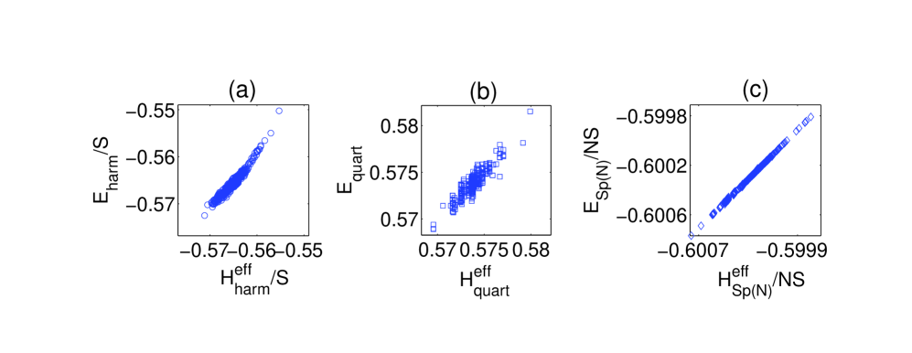
Figure 1: Numerical results for degeneracy-breaking energy versus effective Hamiltonian written in terms of loop; each point represents a different configuration of Ising spins $\{\eta_{i}\}$. (a) Harmonic spin waves (Sec. 2) (b). Quartic spin waves (Sec. 3); only $\pi$-flux states (harmonic ground states) are included. (c) Large-$N$/large-$S$ approximation (Sec. 4).

Most of the retraced path terms are in 1-to-1 correspondence with paths on the coordination-$4$ Bethe lattice. This gave a quite accurate approximation for the constant term $E_{0}$, as well as for the contributions from higher powers of $\boldsymbol{\mu}$ that resum to give each $K_{2l}$ coefficient in (2.2f). Then expanding (2.2e) up to the $l=30$ term [17] (i.e. loops of length $\leq$60), and extrapolating to $n=\infty$, we obtained the coefficients in (2.2f): $E_{0}=-0.5640NS$ , $K_{6}=0.0136S$, $K_{8}=-0.0033S$. To test (2.2f), we numerically computed the zero-point energy (2.1) for many collinear ground states. As confirmed by Fig. 1(a), ${\mathcal{H}^{\mathrm{eff}}}_{\mathrm{harm}}$ represents the energy well.

2.3 Gauge-like symmetry, ground state degeneracy, and discussion

The exact harmonic energy admits “gauge-like” transformations, relating one Ising configuration to another: $\eta^{\prime}_{i(\alpha,\beta)}=\tau_{\alpha}\tau_{\beta}\eta_{i(\alpha,\beta)}$ where $\tau_{\alpha}=\pm 1$ arbitrarily on every diamond site. In matrix notation, $\boldsymbol{\mu}^{\prime}=\boldsymbol{\tau}\boldsymbol{\mu}\boldsymbol{\tau}^{-1}$, where $\boldsymbol{\tau}={\rm diag}(\{\tau_{\alpha}\})$. Then $\boldsymbol{\mu}^{\prime}$ is similar to $\boldsymbol{\mu}$ and has the same eigenvalue spectrum, so $E_{\mathrm{harm}}(\{\eta_{i}\})=E_{\mathrm{harm}}(\{\eta^{\prime}_{i}\})$. These are not literally gauge transformations, since the classical ground-state condition must independently be satisfied: namely, $\sum_{i\in\alpha}\eta_{i}=0$ in every tetrahedron. Since $E_{\mathrm{harm}}$ is gaugelike invariant, its value can only depend on gaugelike invariant combinations of $\{\eta_{i}\}$, i.e. loop products, which explains why (2.2f) has exactly the form of a $Z_{2}$ (Ising) lattice gauge action.

It follows that the harmonic ground states are degenerate; as (2.2f) implies and the numerical calculation confirmed, they are all the (collinear) configurations in which the loop product is $\prod\eta_{i}=-1$ around every hexagon. We call these $\pi$-flux states in the language of Ref. [6]. The divergent modes of Sec. 2.1 provide a trick to construct and count gauge-like transformations and hence the ground state degeneracy. Namely, any gauge-like transformation can be factorized into two, involving the even and odd diamond lattice sites; these transformations in turn correspond one-to-one with a basis of divergent modes. In this fashion, an upper bound [17] on the ground state entropy was obtained, of order $L\ln L$. On the other hand, a lower bound of order $L$ is easily obtained by explicitly constructing a subfamily of $\pi$-flux states by stacking independent layers of thickness $a/4$ in (say) the $[001]$ cubic direction. Each layer is a set of chains running in the $[110]$ or $[1\bar{1}0]$ direction, with spins alternating both along and transverse to the chains, so there is a twofold choice for each layer [16].

Two important loose ends of our harmonic calculation are (i) it was not proven, but only checked numerically [5, 17], that collinear states are local minima of the harmonic zero-point energy (2.1) as a function of classical orientations; nor was it proven that they are the only stationary points. (ii). We do not yet understand the full set of harmonic ($\pi$-flux) ground states for the pyrochlore: only a special subset are given by the layer stacking construction [17].

The (harmonic-order) loop expansion is easily adapted to similar Heisenberg antiferromagnets that support collinear ground states, such as the checkerboard lattice [6]. More interesting are the kagomé or pyrochlore antiferromagnet at a large field “magnetization plateau” [11, 17]: in that case, the signs get reversed in (2.2f). (In the pyrochlore case, with $\uparrow\uparrow\uparrow\downarrow$ tetrahedra, ${\mathcal{H}^{\mathrm{eff}}}_{\mathrm{harm}}$ now favors a positive loop product $\Phi_{6}=+1$.) In each case, the ground state entropy again comes out $O(L)$.

Hassan and Moessner [25] got corresponding results for the ${\mathcal{H}^{\mathrm{eff}}}_{\mathrm{harm}}$ of kagomé antiferromagnets (including noncollinear states) in a (variable) field, uncovering further subtleties of the degeneracies. Also, Bergman et al [11] extended the derivation of  (2.2f) to their easy-axis limit.

3 Anharmonic spin-wave theory

At harmonic order, the pyrochlore antiferromagnet has wriggled loose from our efforts to pin it down to a unique ground state. Evidently, we must try again using the anharmonic terms. As in the kagomé case, brute-force perturbation theory – taking the expectation ${\langle}\mathcal{H}_{\mathrm{quart}}{\rangle}$ in the ground state of $\mathcal{H}_{\mathrm{harm}}$ – fails, since the harmonic fluctuations are divergent. Instead, we must construct a reasonable ground state by using the anharmonic terms self-consistently.

3.1 Self-consistent decoupling

The quartic term $\mathcal{H}_{\mathrm{quart}}$ can be decoupled in a standard fashion: in each quartic term, simply pair the operators and replace one of the pairs by its expectation, in every possible way. The result is a “mean-field” Hamiltonian – quadratic like $\mathcal{H}_{\mathrm{harm}}$, but now all eigenfrequencies are nonzero (except the Goldstone mode) and all divergent modes have been regularized. One can interpret its ground state wavefunction variationally as being the best harmonic-oscillator state for the actual Hamiltonian. The effective nearest-neighbor interactions are modified as

$$J_{ij}\to J_{ij}+\delta J_{ij},\quad\delta J_{ij}=-\frac{1}{S^{2}}\left[\frac{1}{2}\left(G_{ii}+G_{jj}\right)-\eta_{i}\eta_{j}G_{ij}\right].$$ (2.2a)

Here, $G_{ij}\equiv{\langle}\sigma^{x}_{i}\sigma^{x}_{j}{\rangle}\equiv{\langle}\sigma^{y}_{i}\sigma^{y}_{j}{\rangle}$ is the correlation function of fluctuations, which we can evaluate numerically. The anharmonic energy depends on a completely different set of modes than the harmonic energy did. In light of (2.2a), $E_{\mathrm{quart}}$ is dominated by the divergent (at harmonic order) modes introduced in Sec. 2.1; those are zero modes, which do not contribute $E_{\mathrm{harm}}$ at all (recall (2.1)). In principle, then, our recipe is to guess a regularized Hamiltonian, compute its correlations $\{G_{ij}\}$, and insert these in (2.2a) to get a new Hamiltanian; then, iterate until this converges.

3.2 Mean field Hamiltonian and self-consistency

We need to understand the $\{G_{ij}\}$ due to divergent modes. These modes simultaneously enjoy all properties of both ordinary and generic zero modes (since these branches are becoming linearly dependent). We use the fact that any ordinary mode  [17], satisfies

$$v^{(m)}(i)=\frac{1}{\sqrt{2}}\eta_{i}\sum_{\alpha:i\in\alpha}u^{(m)}_{\alpha},$$ (2.2b)

where $\{u^{(m)}_{\alpha}\}$ is the eigenvector of $\{\mu_{\alpha\beta}\}$ having the same eigenvalue $\omega_{m}$, and where the sum runs over both diamond sites linked through pyrochlore site $i$.

Note that as $S\to\infty$, $\mathcal{H}_{\mathrm{quart}}\ll\mathcal{H}_{\mathrm{harm}}$, so we approach a pure harmonic Hamiltonian. In this limit the modes are almost gaugelike-invariant (the regularization breaks the invariance). We may assume the lower-order term $E_{\mathrm{harm}}$ has been minimized, i.e. a $\pi$-flux state. Any such state is specially uniform in that all hexagons are the same, modulo the gauge-like symmetry, and hence all bonds and sites are equivalent, Thus, it turns out, the fluctuations of the diamond-site modes in (2.2b) have correlations with a simple form parametrized by constants ${g}_{1}$,${g}_{2}$, and ${g}_{3}$: ${\langle}u_{\alpha}^{2}{\rangle}={g}_{0}$ (the same on every site); ${\langle}u_{\alpha}u_{\gamma}{\rangle}=\eta_{\alpha\beta}\eta_{\beta\gamma}{g}_{2}$ for second neighbor $(\alpha,\gamma)$ on the diamond lattice, having $\beta$ as their common neighbor (here ${g}_{2}<0$); and (by bipartiteness) ${\langle}u_{\alpha}u_{\beta}{\rangle}=0$ for nearest neighbor $(\alpha,\beta)$. Inserting into (2.2b), we find the correlations are $G_{ii}={g}_{0}$ and $G_{ij}=\frac{1}{2}[\eta_{i}\eta_{j}{g}_{0}+{g}_{2}]$. Substituting this into (2.2a) finally gives

$$\delta J_{ij}=-\frac{1}{2S^{2}}\left({g}_{0}+\eta_{i}\eta_{j}|{g}_{2}|\right)\equiv-\delta J^{*}-\frac{\epsilon}{8}\eta_{i}\eta_{j}.$$ (2.2c)

The constant is absorbed in a re-renormalization to $J^{*}=\tilde{J}(1-\delta J^{*})$; the key (small) parameter is $\epsilon$, which breaks the gauge-like invariance and cuts off the divergences.

Thus, the mean-field Hamiltonian is well approximated by the simple form (2.2c), which in effect says “strengthen the satisfied bonds relative to the unsatisfied bonds.” That is also the simplest possible form of a variational Hamiltonian that is consistent with the local spin symmetries. In practice, we simply assumed (2.2c) and computed ${g}_{2}(\epsilon)$, so the problem reduces to one self-consistency condition, $\epsilon/8=|{g}_{2}(\epsilon)|/2S^{2}$. It turns out $G_{ij}\sim{g}_{2}\sim S\ln\epsilon$, hence $\epsilon\sim\ln{S}/S$ and finally $E_{\mathrm{quart}}\sim(\ln{S})^{2}$. (The log divergence is a consequence of the strongly anisotropic momentum dependence of the modes near the divergence lines in reciprocal space.)

3.3 Effective Hamiltonian, numerical results, and discussion

We calculated the quartic energy numerically for various periodic states, grouped in families within which the states are gaugelike equivalent. They had unit cells ranging from 4 to 32 sites, and five gauge families were represented, in particular the $\pi$-flux states (ground states of ${\mathcal{H}^{\mathrm{eff}}}_{\mathrm{harm}}$). When the result was fitted to an effective Hamiltonian, all but a few percent of the anharmonic energy is actually accounted by gauge-invariant terms, of the same form as (2.2f). The gauge-dependent energy differences between states are much smaller in the $\pi$-flux state, and larger in a gauge family where the gauge-invariant loops are most inhomogeneous. We searched for the optimum among (we believe) all possible $\pi$-flux states in the several unit cells we used (with $N_{s}$ up to $192$ sites).

We performed a numerical fit to an effective Hamiltonian of the form

$${\mathcal{H}^{\mathrm{eff}}}_{\mathrm{quart}}=C_{6}(S)\mathcal{P}_{6}+C_{8}(S)\mathcal{P}_{8}+C_{10}(S)\mathcal{P}_{10}\,,$$ (2.2d)

where $\mathcal{P}_{l}$ is equal to the number of loops of length $l$ composed solely of satisfied bonds (i.e. with alternating spins). Here $C_{6}(100)\approx-0.0621,C_{8}(100)/N_{s}\approx-0.0223.$ (These energies were fitted to $(\ln{S})^{2}$ dependence [18], as implied by the analytics; but our range of $S$ values is too small to distinguish from some other power of $\ln S$.) The scatter plot in Fig. 1(b) shows that the fit (2.2d) captures the leading order dependence on the Ising configuration that splits the harmonic-order degeneracy.

To explain (2.2d) analytically, note the quartic energy is proportional to the energy of (2.2c), evaluated as if it were harmonic. That can be handled by a small generalization of the loop expansion of Sec. 2. The leading state-dependent term turns out to be $\mathcal{P}_{6}$ (with $C_{6}\propto\epsilon^{2}$), confirming analytically a form we had originally conjectured empirically.

The highest and lowest energy states of (2.2d) have, respectively, the smallest and largest numbers of hexagons with spin pattern $\uparrow\downarrow\uparrow\downarrow\uparrow\downarrow$ [20]. The maximum fraction (1/3) of such alternating hexagons is found in a set of states constructed by layering two-dimensional slabs. Within our numerical accuracy, these are degenerate for any $S$. These stacked states have the same number of alternating loops of all lengths up to $16$ (we checked), indeed (we believe) up to $26$. We conjecture a tiny splitting of these states at that high order, maybe even smaller than the similar case of our large-$N$ calculation (see Sec. 4.3, below.)

We also calculated the anharmonic effective Hamiltonian for the (planar) checkerboard lattice, a tractable test-bed for pyrochlore calculations [3, 6, 26]. But, inescapably, two bonds of every “tetrahedron”, (appearing as diagonals of a square) have no symmetry reason to be degenerate with the other four bonds. So, in the anharmonic calculation, the diagonal bonds renormalize to be weaker than the rest, and a unique ordered state is trivially obtained.

Bergman et al [11] developed a quite different derivation of effective Hamiltonians – nicely complementary to ours – by expanding around the Ising limit. Their ${\mathcal{H}^{\mathrm{eff}}}$’s have a form quite like (2.2d) – i.e., the terms count the number of loops with different Ising configurations – and identifying the ground states is comparably difficult. It would have been valuable if we had generalized our anharmonic calculation to the magnetization-plateau case (see end of Sec. 2), to compare with the results of Ref. [11]. (The complication of this generalization is that (2.2c) will get a term with $\eta_{i}+\eta_{j}$, necessitating a second variational parameter in addition to $\epsilon$.)

One naively, but wrongly, expected a similar story for the Heisenberg quantum antiferromagnet on the pyrochlore lattice as on the (previously studied) kagomé lattice [22, 27]. There, spin wave fluctuations selected coplanar (not collinear) configurations as local minima; since all bond angles are $120^{\circ}$, all coplanar states were degenerate to harmonic order unlike our result in Sec. 2.3. Due to the non-collinearity, the counterpart of (2.2) had a term $\mathcal{H}_{\mathrm{cubic}}$, third order in $\{\sigma^{x/y}\}$, and $O(\mathcal{H}_{\mathrm{cubic}}^{2})$ contributed the same order as $O(\mathcal{H}_{\mathrm{quart}})$  [22, 27]. A consequence was distant-neighbor terms in the effective Hamiltonian [27] (which selected the unique “$\sqrt{3}\times\sqrt{3}$” state). A second consequence of non-collinearity was that all generic zero modes – an entire branch – were divergent, and hence in the kagomé case, the anharmonic energies (and squared spin fluctuations) both scaled as $O(S^{2/3})$, much larger than the $(\ln S)^{2}$ of the pyrochlore case.

4 Large-$N$ approach to large-$S$ limit

Besides the spin-wave expansion, there is another systematic approach to go beyond basic mean field theory: Schwinger bosons. Each (generalized) spin has Sp($N$) symmetry and is written as a bilinear in boson operators $\{b_{i\sigma m}\}$, where $\sigma=\uparrow,\downarrow$ and $m$ runs over $N$ flavors; the representation is labeled by $\kappa$ which generalizes $2S$. The physical case is SU($2$) $\cong$ Sp($1$), but the $N\to\infty$ limit can be solved exactly and is often successful as a mean-field theory or the starting point of a $1/N$ expansion; [28] this is popular as an analytic approach to $S=1/2$, in small $\kappa$ limit, since exotic disordered ground states can be represented as well as ordered ones. [28] In our work  [19], (with Prashant Sharma as the major collaborator, who initiated us into this approach) we instead pursued the large-$N$ approach for large $\kappa$. This gives an easier recipe for ground state selection than the spin-wave approach, since in large-$N$ the degeneracies are usually broken at the lowest order [28].

But which saddle point to expand around? In the pyrochlore antiferromagnet, there are exponentially many, corresponding to the same collinear states as in the spin-wave expansion and labeled by the same Ising variables $\{\eta_{i}\}$. Prior studies just investigated high symmetry states, or every state in a small finite system [28, 26]. We pursue instead the effective Hamiltonian approach.

4.1 Large-$N$ mean field theory

Exchange interactions are quadratic in “valence bond” operators $\hat{Q}_{ij}\equiv b^{\dagger}_{i\uparrow,m}b^{\dagger}_{j\downarrow,m}-b^{\dagger}_{i\downarrow,m}b^{\dagger}_{j\uparrow,m}$, and in the boson number operator ${\hat{N}^{\rm b}}_{i}\equiv\sum_{\sigma,m}b^{\dagger}_{i\sigma,m}b_{i\sigma,m}$. (Here $m\leq N$ is a flavor index in the large $N$ generalization, and $\sigma=\uparrow,\downarrow$.) For the physical $SU(2)$ spins, we have $\mathbf{S}_{i}\cdot\mathbf{S}_{j}\to{\hat{N}^{\rm b}}_{i}{\hat{N}^{\rm b}}_{j}-{\hat{Q}}^{\dagger}_{ij}{\hat{Q}}_{ij}$. A decoupling quite generally gives

$$\mathcal{H}_{Sp(N)}=\frac{1}{2}\sum_{\langle ij\rangle}\left(N|Q_{ij}|^{2}+Q_{ij}{\hat{Q}}_{ij}+H.c.\right)+\sum_{i}\lambda_{i}\left({\hat{N}^{\rm b}}_{i}-N\kappa\right)$$ (2.2a)

with the classical numbers $Q_{ij}\equiv{\langle}{\hat{Q}}_{ij}{\rangle}/N$. The Lagrange multipliers $\lambda_{i}$, which (it turns out) have the same value $\lambda=4\kappa$ on every site, enforce the physical constraint that the boson number is exactly $\kappa$ (the generalized spin length) at every site. We want the first nontrivial term in a $1/\kappa$ (semiclassical) expansion.

The desired ordered state is a condensation of bosons, ${\langle}b_{i\sigma,m}{\rangle}=\sqrt{N}\delta_{1,m}x_{i\sigma}$. The mean-field ground state energy, obtained via a Bogoliubov diagonalization, is $E_{Sp(N)}^{\mathrm{tot}}=E_{Sp(N)}^{\mathrm{class}}+E_{Sp(N)}$: the first is the same in every classical ground state. The quantum term is the bosons’ zero-point energy:

$$E_{Sp(N)}=(\{Q_{ij}\})\frac{N}{2}[\Tr{\sqrt{\lambda^{2}\underline{1}-\mathbf{Q}^{\dagger}\mathbf{Q}}}-N_{s}\lambda].$$ (2.2b)

In a collinear classical state, $Q_{ij}=\kappa(\eta_{i}-\eta_{j})/2$, i.e., $\pm\kappa$ for every satisfied bond but zero for unsatisfied bonds.

4.2 Loop expansion and effective Hamiltonian

We have manipulated $E_{Sp(N)}$ into the form of a trace of a matrix square root, as in (2.2e) for the harmonic spin wave energy – but this matrix $\mathbf{Q}$ connects pyrochlore sites $i$, whereas $\boldsymbol{\mu}$ in Sec. 2 connected diamond-lattice sites. A Taylor expansion of (2.2b) gives the desired effective Hamiltonian,

$$E_{Sp(N)}=-\frac{N}{2}\sum_{m=1}^{\infty}\frac{(2m+1)!!}{2^{m}\lambda^{2m-1}m!}\Tr\left(\mathbf{Q}^{\dagger}\mathbf{Q}\right)^{m}$$ (2.2c)

Evidently $\Tr[(\mathbf{Q}^{\dagger}\mathbf{Q}/\kappa^{2})^{m}]$ is just the number of closed paths of length $2m$ on the network of satisfied bonds; this network is bipartite, so every nonzero element of $\mathbf{Q}^{\dagger}\mathbf{Q}$ is $\kappa^{2}$. Those paths that eventually retrace every step can be put in 1-to-1 correspondence with paths on the Bethe lattice (more precisely, a “Husimi cactus” graph [19]). They contribute only a constant factor independent of $\{\eta_{i}\}$ as do paths decorated by additional loops that lie within one tetrahedron. The effective Hamiltonian is a real-space expansion in loops made of valence bonds:

$${\mathcal{H}^{\mathrm{eff}}}_{Sp(N)}=\frac{N\kappa}{2}\left({\tilde{C}}_{0}N_{s}+{\tilde{C}}_{6}\tilde{\mathcal{P}}_{6}+{\tilde{C}}_{8}\tilde{\mathcal{P}}_{8}+\cdots\right)$$ (2.2d)

where $\tilde{\mathcal{P}}_{2l}$ is the number of non-trivial loops of length $2l$ with alternating spins, on (now) the pyrochlore lattice. The coefficients $\{{\tilde{C}}_{2l}\}$ were given as a highly convergent infinite sum, hence could can be evaluated to any accuracy: we got ${\tilde{C}}_{6}=-3.482\times 10^{-3}$, ${\tilde{C}}_{8}=-3.44\times 10^{-4}$, and ${\tilde{C}}_{2l+2}/{\tilde{C}}_{2l}\approx 1/10$, so short loops dominate.

Our large-$N$ loop expansion can be extended to all non-collinear classical ground states [19, 20], with the form of (2.2d) but with generalized $\tilde{\mathcal{P}}_{2l}$. It can be applied the kagomé and checkerboard lattices, [19] giving the usual answers for their ground states [28, 26].

4.3 Numerical results and discussion

We calculated the self-consistent energy for many different collinear classical ground states, obtained by a random flipping algorithm described in Ref. [17]. Eq. (2.2d) is an excellent fit of the state-dependent energy even with just the $2l=6$ and $2l=8$ terms, as shown in Fig. 1(c). An independent numerical fit agreed to within 1% for ${\tilde{C}}_{6}$ and 10% for ${\tilde{C}}_{8}$ [19].

We performed classical Monte Carlo simulations of the Ising model with (2.2d) as its Hamiltonian to systematically search for the ground state, using large orthorhombic unit cells with $128$ to $3456$ sites. The optimum was found for a family of nearly degenerate states built as a stack of layers, so the entropy of this family is $O(L)$. (Each layer has thickness $3a/4$ and there are four choices per layer, but this is not the family found in Sec. 3.) These states are a subset of those with the maximum value $\tilde{\mathcal{P}}_{6}=N_{s}/3$ – i.e., one-third of all $N_{s}$ hexagons are $\uparrow\downarrow\uparrow\downarrow\uparrow\downarrow$ – and $\mathcal{P}_{8}=23N_{s}/6$. However, it turns out a tiny energy difference $\sim 10^{-7}$ per spin, corresponding to the $2l=16$ term in (2.2d), splits these states and selects a unique one.

Let us check our results against the spin-wave approach of Sec. 2. The harmonic term of the $1/S$ expansion must dominate at sufficiently large $S$, so the physical ($SU(2)$) semiclassical ground state must be a ground state of that term, namely a “$\pi$-flux” state. Yet the ground states of (2.2d) are not $\pi$-flux states, and therefore cannot possibly be the true ground state: the $1/N$ expansion has let us down. Nevertheless, if $E_{Sp(N)}$ values are compared within the “gauge” family of $\pi$-flux states, the ordering of these energies is similar to the quartic spin-wave result (Sec. 3).

5 Conclusion

The trick of writing the zero-point energy as the trace of a matrix, (Eqs. (2.2d) and (2.2b)) – and, for the spinwave expansions, transposing to the diamond lattice (Eqs. (2.2c)) and (2.2b)) – enabled an (uncontrolled) expansion giving the effective Hamiltonian in terms of Ising spins as a sum of over loops. In each case, there was a degenerate or nearly degenerate family of states with entropy of $O(L)$. The practical conclusion is clear, at least : beyond harmonic order, energy differences are ridiculously small and would not be observed in experiments.

Is it, then, possible to realize a disordered superposition of these states, once we add to our effective Hamiltonian the “off-diagonal” terms, representing the amplitudes for tunneling between collinear states? (Compare [13] for the kagomé case, and [11] for the pyrochlore.) Unfortunately, the $O(L)$ entropy of ground states implies that transition from one to another requires flipping $O(L^{2})$ spins, so the tunnel amplitude is exponentially small as $L\to\infty$. One also noticed that collinear selection (mentioned before Sec. 2.1) provides a different route than “spin ice” to realize an effective Ising model in a pyrochlore system; when these collinear states are allowed tunnelings (i.e. ring exchanges), won’t we realize the “$U(1)$ spin liquid” of  [29]? To stabilize a quantum superposition, the tunnel amplitude should be larger than the energy splittings among collinear states, but smaller than the energy favoring collinearity – yet in the pyrochlore, both energy scales are comparable (of harmonic order, i.e. relative order $1/S$). The kagomé lattice – or in $d=3$, the garnet lattice of corner-sharing triangles – is far more promising for disordered spin states, since its harmonic-order ground states have extensive entropy.

References

References

- [1] R. Moessner and A. P. Ramirez, Phys. Today 59, 24 (2006).
- [2] J. E. Greedan, J. Mater. Chem. 11, 37 (2001).
- [3] R. Moessner and J. T. Chalker, Phys. Rev. B 58, 12049 (1998).
- [4] B. Canals and C. Lacroix, Phys. Rev. Lett. 80, 2933 (1998); Phys. Rev. B 61, 1149 (2000).
- [5] H. Tsunetsugu and Y. Motome, Phys. Rev. B 68, 060405 (2003).
- [6] O. Tchernyshyov, J. Phys.: Condens. Matter 16, S709 (2004).
- [7] J. D. M. Champion, A. S. Wills, T. Fennell, S. T. Bramwell, J. S. Gardner, and M. A. Green, Phys. Rev. B 64, 140407 (2001).
- [8] S.-H. Lee, C. Broholm, T. H. Kim, W. Ratcliff, and S-W. Cheong, Phys. Rev. Lett. 84, 3718 (2000);
- [9] O. Tchernyshyov, Phys. Rev. Lett. 93, 157206 (2004).
- [10] L. Santos, M. A. Baranov, J. I. Cirac, H.-U. Everts, H. Fehrmann, and M. Lewenstein, Phys. Rev. Lett. 93, 030601 (2004).
- [11] D. L. Bergman, R. Shindou, G. A. Fiete, and L. Balents, Phys. Rev. Lett. 96, 097207 (2006); cond-mat/0607210,
- [12] C. L. Henley, Can. J. Phys. 79, 1307 (2001).
- [13] J. von Delft and C. L. Henley, Phys. Rev. B 48, 965 (1993).
- [14] O. Tchernyshyov, R. Moessner, and S. L. Sondhi, Europhys. Lett. 73, 278 (2006).
- [15] B. Douçot and P. Simon, J. Phys. A: Math. Gen. 31, 5855 (1998).
- [16] C. L. Henley, Phys. Rev. Lett. 96, 047201 (2006).
- [17] U. Hizi and C. L. Henley, Phys. Rev. B 73, 054403 (2006).
- [18] U. Hizi and C. L. Henley, preprint (2006) “Anharmonic ground state selection in the pyrochlore antiferromagnet”.
- [19] U. Hizi, P. Sharma, and C. L. Henley, Phys. Rev. Lett. 95, 167203 (2005).
- [20] U. Hizi, Ph.D. thesis, Cornell University (2006).
- [21] A.B. Harris, A. J. Berlinsky, and C. Bruder, J. Appl. Phys. 69, 5200 (1991).
- [22] A. V. Chubukov, Phys. Rev. Lett. 69, 832 (1992).
- [23] E. F. Shender, Sov. Phys. JETP, 56, 178 (1982).
- [24] C. L. Henley, Phys. Rev. Lett. 62, 2056 (1989).
- [25] S. R. Hassan and R. Moessner, Phys. Rev. B 73, 094443 (2006).
- [26] J.-S. Bernier, C.-H. Chung, Y. B. Kim, and S. Sachdev, Phys. Rev. B 69, 214427 (2004).
- [27] C. L. Henley and E. P. Chan, J. Magn. Magn. Mater. 140, 1693 (1995); E. P. Chan, Ph.D. thesis, Cornell University (1994).
- [28] S. Sachdev, Phys. Rev. B 45, 12377 (1992), and references therein.
- [29] M. Hermele, M. P. A. Fisher, and L. Balents, Phys. Rev. B 69, 064404 (2004).