Effects of short-range interactions on transport through quantum point contacts:
A numerical approach

Abstract

We study electronic transport through a quantum point contact, where the interaction between the electrons is approximated by a contact potential. Our numerical approach is based on the non-equilibrium Green function technique which is evaluated at Hartree-Fock level. We show that this approach allows us to reproduce relevant features of the so-called “0.7 anomaly” observed in the conductance at low temperatures, including the characteristic features in recent shot noise measurements. This is consistent with a spin-splitting interpretation of the process, and indicates that the “0.7 anomaly” should also be observable in transport experiments with ultracold fermionic atoms.

I Introduction

One of the most prominent quantum phenomena in mesoscopic physics is the effect of conductance quantization. The conductance of a quantum point contact measured as a function of an applied gate voltage exhibits plateaus at integer multiples of the conductance quantum, $G_{0}=2e^{2}/h$, where $-e$ is the electron charge and $h$ is Planck’s constant Wee88 ; Wha88 ; Khu88 . These steps are well understood in terms of non-interacting electrons Bee91 . But experimental conductance curves frequently show an additional plateau-like feature below the first conductance step at a value around $0.7\times G_{0}$. This so-called “0.7 anomaly” was first investigated experimentally by Thomas et al. Tho96 who particularly looked at the magnetic field- and temperature dependence of the additional plateau. They found that the 0.7-feature develops smoothly into the Zeeman spin-split plateau at $0.5\times G_{0}$ by applying a parallel in-plane magnetic field. That is why those authors related this anomaly to the spin degree of freedom of the electrons. They conjectured the presence of spin polarization in quasi one-dimensional junctions. In addition, Thomas and coworkers revealed that the 0.7 plateau becomes more pronounced if the temperature is increased.

Since those first measurements there has been much experimental Tho98 ; Kri00 ; Nut00 ; Rei01 ; Cro02 ; Rei02 ; Roc04 ; Rok06 ; Dic06 and theoretical Wan96 ; Bru01 ; Ber02 ; Mei02 ; Hir03 ; See03 ; Sta03 ; Ber05 ; Rei05 ; Rei06 ; Gol06 ; Rej06 ; Ber06 effort to explain the origin of this effect. However, a complete understanding is still missing. Experiments show a zero-bias peak in the differential conductance typical for the Kondo effect Cro02 . Furthermore, the temperature dependence can be characterized by a single parameter which was interpreted as the Kondo temperature. In a recent experiment Rok06 a static spin polarization was measured, which contradicts the Kondo interpretation. Shot noise measurements Roc04 ; Dic06 could show that two differently transmitting channels contribute to transport.

Theoretical studies of this phenomenon are, on the one hand, based on calculations using density functional theory (DFT), Ber06 ; Wan96 ; Ber02 ; Sta03 ; Ber05 . In an early publication Wang and Berggren showed how Coulomb interaction can split the energy levels of up- and down electrons in a quasi one-dimensional system Wan96 . They used DFT calculations with Hartree- and exchange potentials in local density approximation. Their findings were confirmed by more sophisticated calculations which include exchange-correlation potentials and take into account realistic gate potentials Ber02 ; Sta03 ; Ber05 . The observed difference of the up- and down energy levels gives rise to spin dependent transmissions which manifest themselves in a 0.7 feature in the total conductance. However, to our knowledge there are no DFT results showing the correct temperature dependence.

Besides DFT calculations, there are various theoretical models describing different aspects of the 0.7 anomaly. Some models are based on the presence of spin-splitting Bru01 ; Rei05 ; Rei06 , assuming a density dependent separation of the up- and down energy levels from the beginning. These models can qualitatively reproduce the correct magnetic field and temperature dependence of the 0.7 structure and are also suitable to describe shot noise Dic06 . In a complementary approach the 0.7 anomaly is related to the Kondo effect Mei02 ; Hir03 by treating the quantum point contact as an interacting two-level system for the different spins. Qualitatively, this approach also leads to the observed temperature and magnetic field behavior of the 0.7 feature Cro02 . Very recently, also shot noise was calculated within this model showing agreement with experimental data Gol06 . Furthermore, interaction with phonons is used to explain the unusual temperature dependence See03 .

In this work we present a comparatively simplified approach to the problem, which is based on the non-equilibrium Green function technique where the interaction is incorporated at the Hartree-Fock level. We shall, furthermore, approximate the screened Coulomb interaction between the electrons by a repulsive contact potential. The fact that we can, within this approach, reproduce all relevant features of the 0.7 anomaly at temperatures close to zero, including the recently observed modification of the shot noise factor Dic06 , supports arguments in favor of the spin-splitting mechanism Wan96 ; Ber02 ; Sta03 ; Ber05 ; Bru01 ; Rei05 ; Rei06 (in line with experimental evidence provided in Ref. Rok06 ) and indicates that the effect is rather robust with respect to the precise theoretical description of the process. The short-range potential is furthermore chosen with regard to possible future transport experiments of ultracold fermionic atoms which precisely interact via the contact potential that we are using.

This paper is organized as follows: in Section II we introduce our model and present the relevant expressions that are used to calculate the transport properties. We show our numerical results in Section III where we concentrate on the influence of the coupling constant and the magnetic field on the conductance. We discuss the zero field case and show results concerning shot noise and finite temperatures. In Section IV we summarize our results and discuss transport of fermionic atoms through a constriction. The Appendix consists of a part about determining the strength of the interaction constant and other model parameters in an ideal two-dimensional electron gas. Another part contains a detailed description of how to extend the recursive Green function algorithm to non-equilibrium processes.

II The Model

We describe a two-dimensional electron system with an additional in-plane confinement potential $V_{\rm conf}(x,y)$ that defines the geometry of the quantum point contact. The in-plane magnetic field $\vec{B}=(B,0,0)$ oriented towards the transport direction gives rise to a Zeeman term only. For moderate magnetic fields the orbital contribution vanishes with the choice $\vec{A}=(0,-Bz,0)$ for the vector potential and $z=0$ for the location of the two-dimensional electron gas (2DEG). Therefore, the non-interacting part of the Hamiltonian of the system can be written as

$$H_{0}^{\sigma}=\frac{p_{x}^{2}+p_{y}^{2}}{2m}+V_{\rm conf}(x,y)+g\mu_{B}B\sigma,$$ (1)

where $m$ is the effective mass and $\sigma=\pm 1/2$ is the spin quantum number. The spin-up and spin-down energy levels are separated by the Zeeman energy $E_{Z}=g\mu_{B}B$, where $g$ is the effective gyro-magnetic ratio and $\mu_{B}$ the Bohr magneton. Within our model the interaction of two particles located at $\vec{r}$ and $\vec{r}\,^{\prime}$ is described by

$$V_{\rm int}(\vec{r},\vec{r}\,^{\prime})=\gamma\,\delta(\vec{r}-\vec{r}\,^{\prime}),$$ (2)

with interaction strength $\gamma$. This choice of the interaction can be interpreted as a simple model for an efficiently screened Coulomb potential. For a homogeneous 2DEG the Thomas-Fermi screening length is of the order $\lambda_{s}\approx 5\;\rm nm$ and the width of a typical constriction is roughly $W\approx 20\;\rm nm$, see Appendix A. Therefore, we do not expect that our model gives an accurate description of the interaction. But it provides a transparent physical picture of the mechanism causing spin splitting. Moreover, our Hamiltonian is particularly devised to predict transport features of neutral fermionic atoms, as discussed in section IV. In that case it is a very good approximation to use delta-like interactions.

The coupling constant $\gamma$ can be estimated by calculating the total interaction energy for a screened Coulomb potential in Thomas-Fermi approximation, as done in Appendix A. We find that $\gamma\simeq 2\pi\times\hbar^{2}/(2m)$ gives a realistic order of magnitude for the interaction strength.

To calculate the transport properties of the system we use the Keldysh Green function approach Dat95 ; Ram86 . This approach is very general as it allows to treat interactions and to include finite temperatures and bias voltages. The physical properties are obtained from the retarded and lesser Green function, $G^{r}$ and $G^{<}$. The former can be used to calculate properties such as the conductance, see Eq. (8); from the latter we get the particle density, see Eq. (5). Within the Green function approach the interaction is treated in a self-consistent way and can be included via a proper self-energy. For our calculations we take into account the first order of the perturbation expansion. The corresponding retarded self-energy is usually written as a sum of the Hartree and Fock self-energies, $\Sigma^{\sigma}_{H}$ and $\Sigma^{\sigma}_{F}$, and has the form Dat95

$$\Sigma^{\sigma}_{H}(\vec{r},\vec{r}\,^{\prime}) = \frac{-\rm i}{2\pi}\;\delta(\vec{r}-\vec{r}\,^{\prime})\sum_{\tilde{\sigma}}\int\negthickspace{\rm d}\vec{r}\,^{\prime\prime}\negthickspace\int\negthickspace{\rm d}E\;V_{\rm int}(\vec{r},\vec{r}\,^{\prime\prime})\times$$ (3)

$$\times\,G^{<}_{\tilde{\sigma}}(\vec{r}\,^{\prime\prime}\negthickspace,\vec{r}\,^{\prime\prime}\negthickspace,E),$$

$$\Sigma^{\sigma}_{F}(\vec{r},\vec{r}\,^{\prime}) = \frac{\rm i}{2\pi}\int{\rm d}E\;V_{\rm int}(\vec{r},\vec{r}\,^{\prime})\;G^{<}_{\sigma}(\vec{r},\vec{r}\,^{\prime}\negthickspace,E).$$

In general, the Hartree self-energy is local, and it involves a sum over all spin directions, whereas the Fock self-energy is non-local and depends only on the lesser Green function of the same spin orientation. However, in our case of delta-interactions, Eq. (2), both the Hartree and the Fock contribution are local. $\Sigma^{\sigma}_{F}$ exactly compensates the $(\sigma=\tilde{\sigma})$-term of the spin sum in $\Sigma^{\sigma}_{H}$, and we easily obtain for the total interaction self-energy

$$\Sigma^{\sigma}_{\rm int}(\vec{r})=\Sigma^{\sigma}_{H}+\Sigma^{\sigma}_{F}=\gamma\;n_{-\sigma}(\vec{r}).$$ (4)

Here,

$$n_{\sigma}(\vec{r})=-\frac{\rm i}{2\pi}\int{\rm d}E\;G^{<}_{\sigma}(\vec{r},\vec{r},E)$$ (5)

is the density of electrons with spin $\sigma$.

The Hamilton operator of the interacting system, $\mathcal{H}^{\sigma}=H^{\sigma}_{0}+\Sigma^{\sigma}_{\rm int}(\vec{r})$, is a sum of the non-interacting Hamiltonian (1) and the interaction self-energy (4), which acts like an additional local potential. This potential is different for the different spin directions: a spin-up electron encounters a potential which is proportional to the density of spin-down electrons, and vice versa. Hence, there is a repulsive interaction only between particles with opposite spin directions. Therefore, any small imbalance between the density of up- and down electrons is increased by this kind of interaction.

To solve the transport problem we discretize the spatial coordinates. The derivatives in the Hamiltonian are then written as finite differences, and the Hamilton operator is represented by a block-diagonal matrix Fru04 . The diagonal matrix elements contain an on-site energy and all local potentials $\mathcal{H}^{\sigma}_{ii}=4\hbar^{2}/(2ma^{2})+V_{\rm conf}(\vec{r}_{i})+\Sigma_{\rm int}(\vec{r}_{i})+g\mu_{B}B\sigma$ (with $a$ the lattice constant). The off-diagonal matrix elements for neighboring sites $i$ and $j$ are $\mathcal{H}_{ij}=-\hbar^{2}/(2ma^{2})$ and zero otherwise. As shown in Fig. 1, the geometry of our system has the shape of a linear constriction with a hard-wall confinement potential $V_{\rm conf}(x,y)$ which is zero inside the scattering region, and infinite outside.

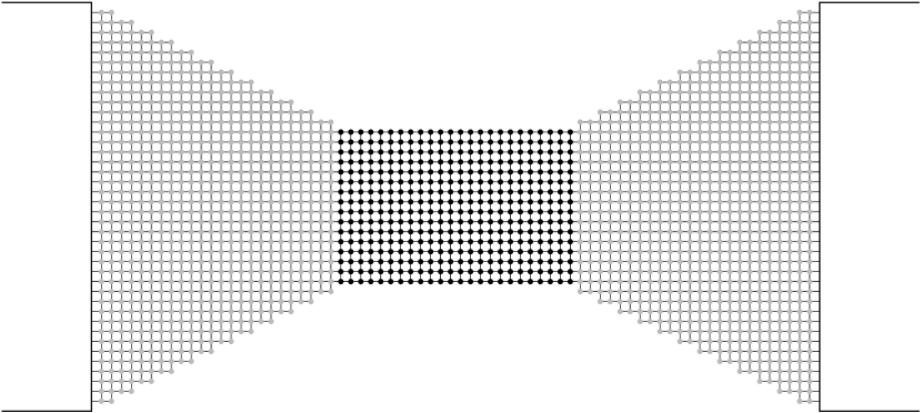
Figure 1: The geometry of the system. Each point corresponds to one site of the numerical grid; the grey points indicate the region where the interaction is gradually switched on and off. The leads are coupled to the left and to the right as indicated by the white bars.

Moreover, the system is coupled to semi-infinite leads that have the same width as the outer slices of the constriction. The leads are in thermal equilibrium characterized by the chemical potential $\mu$, and there is no effective electron-electron interaction in the leads. The interaction potential is gradually switched on/off in the narrowing region indicated by the grey points in Fig. 1. The coupling to the leads can be exactly taken into account by self-energies $\Sigma_{L}$ and $\Sigma_{R}$ for the left and right lead, respectively Dat95 ; Fer97 . With these ingredients it is possible to calculate the full retarded Green function by matrix inversion

$$G_{\sigma}^{r}(E)=\left[E-H^{\sigma}_{0}-\Sigma^{\sigma}_{\rm int}-\Sigma_{L}-\Sigma_{R}\right]^{-1},$$ (6)

where $H^{\sigma}_{0}$ is given in Eq. (1). The Green function is a matrix of dimension $2N\times 2N$, where $N$ is the number of lattice sites. Hence it would be very time consuming to invert the complete matrix in one step, as the computing time scales like $N^{3}$. However, it is possible to implement a recursive algorithm that calculates the Green function of single slices of the scattering region and couples the slices via a Dyson equation. The details of this algorithm are explained in Appendix B. The recursive scheme scales with the third power of the width and only linearly with the length of the system. Thereby it is much more efficient than a direct matrix inversion.

From the retarded Green function we get the lesser function using the kinetic equation

$$G^{<}_{\sigma}(E)=G_{\sigma}^{r}(E)\;\Sigma^{<}(E)\;G_{\sigma}^{a}(E),$$ (7)

where the advanced Green function is obtained by hermitian conjugation, $G_{\sigma}^{a}=[G_{\sigma}^{r}]^{\dagger}$. The lesser self-energy is $\Sigma^{<}(E)=-2{\rm i}\,f(E,\mu)\,{\rm Im}(\Sigma_{L}+\Sigma_{R})$, where $f(E,\mu)$ is the Fermi-Dirac function. This relation holds as the leads are assumed to be in thermal equilibrium. So the lesser self-energy can be interpreted as the in-scattering rate for particles with energy $E$ at a chemical potential $\mu$. The lesser Green function $G^{<}_{\sigma}(E)$ determines the particle density and hence the interaction self-energy, according to Eqs. (4) and (5). Thus, the interaction self-energy can be calculated from the retarded Green function, but in turn the retarded Green function depends on the interaction self-energy. Hence, Eqs. (4) and (6) have to be solved simultaneously.

The solution is carried out in an iterative way: we start with an initial guess for the interaction self-energy to calculate the retarded Green function with Eq. (6). From this we get the lesser Green function, Eq. (7), and combining Eqs. (4) and (5) we obtain a new value for the interaction self-energy. We continue with this scheme until we have reached convergence. As soon as we have found a self-consistent solution we can calculate the conductance of the system using the Landauer formula

$$G=\frac{2e^{2}}{h}{\rm Tr}\Bigl{\{}\Gamma_{L}G^{r}\;\Gamma_{R}G^{a}\Bigr{\}},$$ (8)

with $\Gamma_{L/R}={\rm i}\left(\Sigma_{L/R}-\Sigma_{L/R}^{\dagger}\right)$.

III Numerical Results

III.1 Dependence on the coupling strength

We first calculate the conductance of the previously described model for zero temperature. It is convenient to use as the energy unit $E_{1}=\hbar^{2}\pi^{2}/(2mW^{2})$, the energy of the first transverse mode in the narrow region of the scatterer of width $W$. To break the symmetry between electrons with different spins we apply a small magnetic field so that the Zeeman energy has a value $E_{Z}=g\mu_{B}B=0.0015\;E_{1}$. The case of zero magnetic field is discussed separately in section III.3.

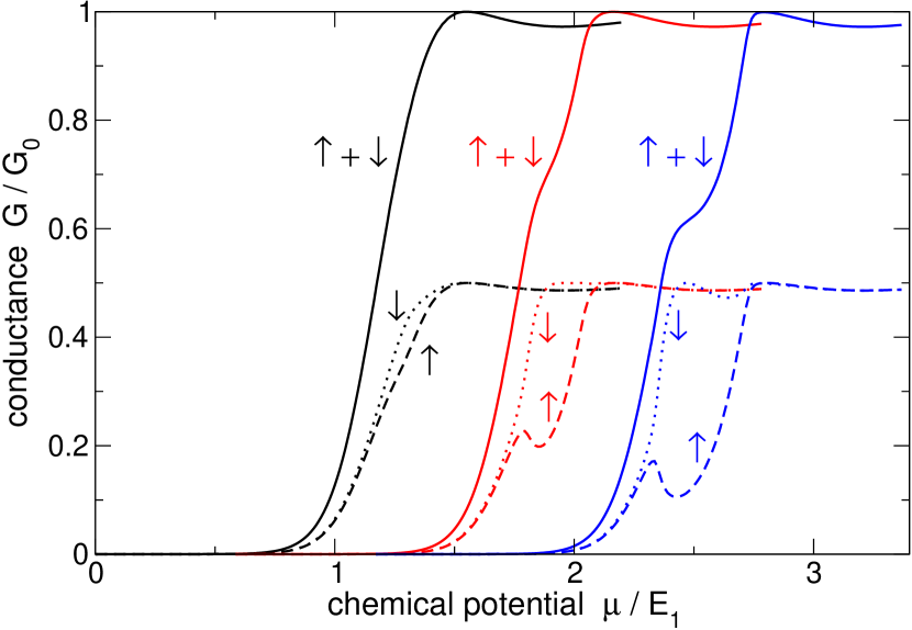
Figure 2: (Color online) Total conductance (solid line) and the up- (dashed) and down (dotted) contributions for different interaction constants $\gamma$. The coupling constant takes values $\gamma=3.7$ (black), $\gamma=4.1$ (red), and $\gamma=4.5$ (blue) from left to right in units of $\hbar^{2}/(2m)$. The curves for $\gamma\geq 4.1$ have been horizontally offset for clarity.

The conductance for different interaction strengths $\gamma$ is shown in Fig. 2. We find that for a small coupling constant $\gamma=3.7\times\hbar^{2}/(2m)$ the up- and down contribution $G_{\uparrow}$ and $G_{\downarrow}$ differ from each other. This difference is not due to the Zeeman shift, as the Zeeman energy is approximately two orders of magnitude lower. It is caused by the effective repulsive interaction between electrons with different spin orientations. If the interaction strength is increased the up- and down contributions split more and more. Additionally, a small shoulder develops in the curve for the total conductance at values between $0.6$ and $0.7$ of the conductance quantum. This is in agreement with experimental results for the 0.7 anomaly in Ref. Tho96 . For sufficiently high interaction constants the contribution of one spin component to the conductance drops down while increasing the chemical potential. These spin-resolved conductance curves coincide with results obtained from transmission across a saddle potential in the presence of a Gaussian spin-splitting Nut00 , and with corresponding DFT results Ber02 .

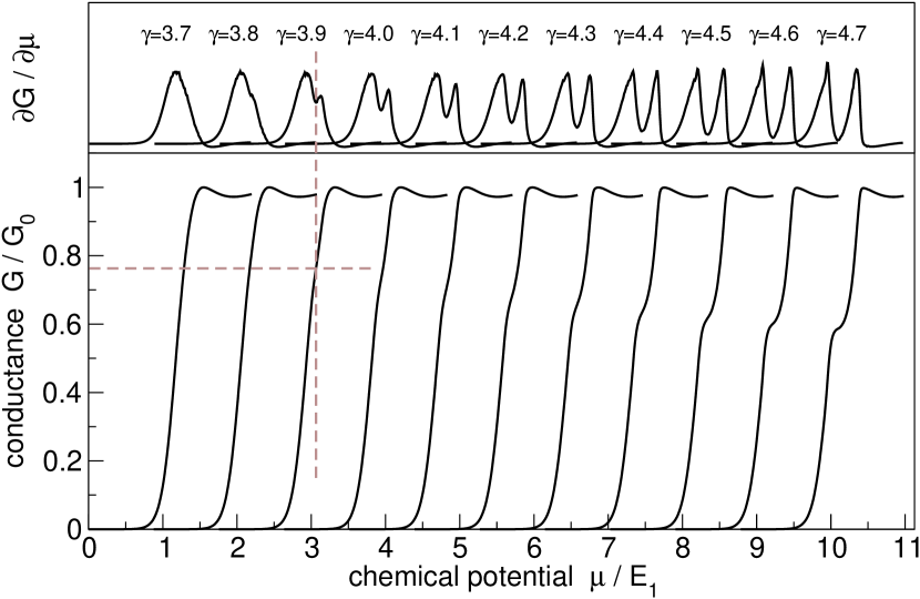
Figure 3: Lower panel: conductance curves for different values of the coupling constant ($\gamma$ is given in units of $\hbar^{2}/(2m)$). The derivative (in arbitrary units) of each curve is plotted straight above the particular graph. The dashed lines mark the conductance value of the “plateau” for the lowest value of $\gamma$, where a local minimum in $\partial G/\partial\mu$ is visible. The different curves are offset horizontally.

The curves in Fig. 2 already indicate that the spin-splitting has to be sufficiently strong in order to get a visible effect in the total conductance. This is in accordance with the experimental results in Ref. Rok06 where the authors measure spin resolved contributions to the total conductance of a point contact. They find that even in samples that are not exhibiting a 0.7 feature the spin-up and -down electrons contribute differently to the total conductance. Fig. 3 shows how the 0.7 plateau develops upon increasing the coupling strength $\gamma$. The lower panel shows the conductance curves and the upper panel the corresponding derivatives $\partial G/\partial\mu$. The derivatives change from a single peak to a double peak shape as the 0.7 plateau develops. The second peak in the derivative appears at a coupling constant $\gamma\approx 3.9\times\hbar^{2}/(2m)$; the corresponding value for the plateau is $G\approx 0.76\;G_{0}$. Increasing the interaction constant, the plateau gets more and more pronounced and eventually converges towards $G_{0}/2$. Hence, in our model the interaction parameter $\gamma$ governs the position and the width of the 0.7 plateau. The higher the conductance value at the plateau, the smaller is its width. There is no plateau above $0.76\;G_{0}$ in our model.

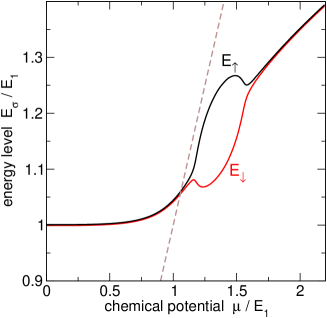
Figure 4: (Color online) Energy levels $E_{\uparrow}$ (black) and $E_{\downarrow}$ (red) for $\gamma=4.5\times\hbar^{2}/(2m)$ and $E_{Z}=0.0015\;E_{1}$. The dashed curve shows the chemical potential $\mu$.

To get information about the energy levels of the different spin orientations we calculate $E_{\sigma}=E_{1}^{\sigma}+\langle\Sigma^{\sigma}_{\rm int}\rangle$. The energy levels of non-interacting electrons $E_{1}^{\sigma}=E_{1}+g\mu_{B}B\sigma$ are shifted by the average interaction potential $\langle\Sigma^{\sigma}_{\rm int}\rangle$ felt by a particle with spin $\sigma$. The brackets $\langle\ldots\rangle$ denote a spatial average over the region with full electron-electron interaction (black points in Fig. 1). The resulting curves in Fig. 4 show that the energy levels $E_{\sigma}$ are located around $E_{1}$ for $\mu=0$. They are very weakly split by the Zeeman energy. With increasing $\mu$ the levels rise in energy as the constriction is populated with electrons and then start to split distinctly, as soon as the chemical potential is comparable with the energy levels $E_{\sigma}$. The reason is that due to the Zeeman splitting the down-level is populated already at a lower chemical potential causing an imbalance between the density of spin-up and spin-down carriers in the constriction. The repulsive interaction between opposite spins tends to increase any imbalance. A small excess of down electrons repels up electrons from the constriction, which results in a larger excess of down particles.

The spin-splitting vanishes when the chemical potential is well above both energy levels. In the range of the chemical potential where the up- and down energy levels are split, also the up- and down contribution to the conductance differs, as shown in Fig. 2. The obtained energy levels shown in Fig. 4 are in line with DFT results Ber02 .

Before comparing with the spin-splitting models Bru01 ; Rei05 we shall note that the quantities plotted in Fig. 4 are only estimations for the energy levels. Due to the geometry of our system the transverse modes are broadened with a width of the order of $E_{1}/2$, as can be seen in the conductance curves of Fig. 2. Therefore, our results seem to confirm the assumption of the spin-splitting models, that the energy levels start to split as soon as the chemical potential crosses the up- and down energy levels. Additionally, we observe a “pinning” of the upper energy level to the chemical potential within a substantial range of $\mu$, that means $E_{\uparrow}$ evolves parallel to the chemical potential $\mu$ right after the splitting. The presence of this level pinning is essential in the spin-splitting models in order to get a 0.7-plateau. In our calculations the plateau also appears in the range where level pinning is present.

III.2 Magnetic field dependence

The shape of the conductance curves is influenced by the magnetic field. Fig. 5 shows that the 0.7 plateau evolves from a small shoulder at $G\approx 0.65\;G_{0}$ to a wide plateau at $G=0.5\;G_{0}$ as the magnetic field is increased. This is in agreement with experiments Tho96 ; Rok06 . In the high-field limit Zeeman splitting is the dominant effect. The energy levels of the different spins are separated by the Zeeman energy which causes a plateau at $0.5\;G_{0}$ even in the case of non-interacting electrons. The reason is that spin-down electrons contribute to transport at chemical potentials $\mu\gtrsim E_{1}-g\mu_{B}B$, whereas for spin-up electrons $\mu\gtrsim E_{1}+g\mu_{B}B$ has to be fulfilled. For strong magnetic fields the effect of electron-electron interaction is only to broaden the Zeeman spin-split plateau at one half of the conductance quantum.

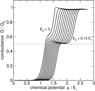
Figure 5: Conductance curves for $\gamma=4.5\times\hbar^{2}/(2m)$ and different magnetic fields. The corresponding Zeeman energies vary from $0$ to $0.14\;E_{1}$ in steps of $0.012\;E_{1}$ from left to right. The curves are horizontally offset.

For a more quantitative comparison between our results and experimental data it is useful to re-scale our quantities and give the magnetic fields in units of Tesla. Therefore, we have to associate an energy value with $E_{1}=\hbar^{2}\pi^{2}/(2mW^{2})$. If we insert the approximate width $W=\sqrt{2/(\pi n)}$ of a quantum point contact from Eq. (15) we get

$$B=\frac{1}{g\mu_{B}}E_{Z}\approx\frac{\hbar\pi^{3}n}{2ge}\frac{E_{Z}}{E_{1}}.$$ (9)

The maximum field applied in Fig. 5 then corresponds to $B\approx 5.8\,\rm T$ where we used $g=0.44$ for bulk GaAs and a density of $n=1.8\times 10^{11}\,\rm cm^{-2}$ Tho96 . This magnetic field value is lower than in experiments where fields of about $10\,\rm T$ are necessary to get a plateau at $0.5\;G_{0}$ Tho96 .

III.3 The zero-field case

For the previous calculations we always applied a finite magnetic field. Due to this field the energy levels of the electrons with different spins were separated so that the down state can be populated at smaller chemical potentials than the up state. That is the reason why up electrons are repelled from entering the constriction, as down electrons are already present at a lower chemical potential. So the repulsive interaction between particles with opposite spins leads to an enhancement of an initially small asymmetry between the density of up- and down electrons in the constriction.

However, in the case of zero magnetic field the Hamiltonian (1) together with the interaction self-energy (4) is strictly symmetric with respect to spin-up and spin-down. Therefore, the resulting conductance curves also have to show the same symmetry. The result for $B=0$ and $\gamma=4.5\times\hbar^{2}/(2m)$ is displayed as the dashed curves in Fig. 6. As expected the contributions of the up- and down electrons exactly coincide and the total conductance has no additional features below the first step.

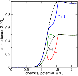
Figure 6: (Color online) Conductance in the zero-field case. The dashed lines are for $B=0$; there is no difference between the $\uparrow$ and $\downarrow$-contribution and the total conductance does not exhibit a 0.7 feature. The solid lines show the results for $B\to 0$ where the $\uparrow$ (red) and $\downarrow$ (green) contributions differ and the total conductance (bold blue line) has a shoulder at $G\approx 0.65\;G_{0}$.

We can investigate the stability of the symmetric solution by slightly disturbing the symmetry of the system. For each point calculated we start with a small magnetic field $E_{Z}^{0}=0.0015\;E_{1}$. During the first four steps of the self consistency loop we turn off the magnetic field according to $E_{Z}^{0}/s$ where $s$ is the number of the iteration step. After four steps we set the magnetic field exactly to zero and continue iterating until the results are converged. In that way we obtain an asymmetric solution for the spin-up and spin-down contributions. In contrast to the finite field results depicted in Fig. 2, here the splitting sets in abruptly at a chemical potential $\mu=1.20\;E_{1}$. In the range where $G_{\uparrow}$ and $G_{\downarrow}$ are different a shoulder appears in the total conductance $G$. Those points where the spin-splitting is absent coincide with the points for $B=0$. So the symmetric solution with $G_{\uparrow}=G_{\downarrow}$ is unstable and we find a 0.7 anomaly even in the case of zero magnetic field.

In our case the down-contribution to the conductance dominates when we apply a positive magnetic field. With a negative field the different spin directions would change their roles. In reality the asymmetry between spin-up and spin-down may be caused by residual magnetic fields or temporal current fluctuations. Also magnetic impurities, as well as nuclear spins and dynamic nuclear polarization might play a role in breaking the up- and down-symmetry. Our numerical results show that a very weak asymmetry is sufficient to get spin-splitting. We obtained spin-split results for Zeeman energies down to $E_{Z}=3\times 10^{-7}\;E_{1}$, corresponding to a magnetic field strength of about $B\approx 10^{-5}\,\rm T$.

III.4 Shot noise

In recent experiments shot noise was measured in quantum point contacts exhibiting a 0.7 anomaly Roc04 ; Dic06 . In the framework of Landauer-Büttiker theory the shot noise power $S$ in a two-terminal device is given by Bla00

$$S=\frac{2e^{2}}{h}\sum_{n,\sigma}\int{\rm d}E\;T_{n,\sigma}(E)\Big{(}1-T_{n,\sigma}(E)\Big{)}\left(f_{L}-f_{R}\right)^{2}.$$

Here, $f_{L/R}$ is the Fermi distribution function of the left/right contact. If the energy scale on which the transmission functions $T_{n,\sigma}(E)$ vary is large compared to temperature $k_{B}T$ and applied source-drain voltage $eV_{\rm sd}$, the transmissions can be treated as constants. Then the energy integral over the distribution functions can be performed, yielding

$$S=2\mathcal{N}\frac{2e^{2}}{h}\left[eV_{\rm sd}\coth\left(\frac{eV_{\rm sd}}{2k_{B}T}\right)-2k_{B}T\right],$$ (10)

with the noise factor defined as

$$\mathcal{N}=\frac{1}{2}\sum_{n,\sigma}T_{n,\sigma}(1-T_{n,\sigma}).$$ (11)

The noise factor of one single channel vanishes for zero or perfect transmission, and it is maximal for $T_{n,\sigma}=1/2$.

By simultaneous noise and conductance measurements it is possible to extract information about spin-resolved transmission coefficients $T_{\uparrow}$ and $T_{\downarrow}$. Whereas the conductance is proportional to the total transmission, $T_{\rm tot}=T_{\uparrow}+T_{\downarrow}$, the noise factor in the single mode case is $\mathcal{N}=\frac{1}{2}T_{\rm tot}(1-T_{\rm tot})+T_{\uparrow}T_{\downarrow}$. Only in the case of non-interacting particles where $T_{\uparrow}=T_{\downarrow}=T$ the noise factor reduces to $\mathcal{N}=T(1-T)$.

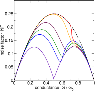
Figure 7: (Color online) Noise factor for $\gamma=4.0\times\hbar^{2}/(2m)$ and for different values of the magnetic field $E_{Z}/E_{1}=$ 0.0, 0.0007, 0.006, 0.012, 0.018, 0.23 from top to bottom. The dashed line indicates the result for non-interacting electrons.

The authors of Ref. Dic06 measured the shot noise power and fitted their experimental results with Eq. (10) using $\mathcal{N}$ as fitting parameter. They find a suppression of noise around the anomalous conductance plateau. That gives experimental evidence that near the 0.7 feature electrons are transported by two channels with different transmissions, as also stated in Roc04 . This agrees with our results for $G_{\uparrow}$ and $G_{\downarrow}$ displayed in Fig. 2. For conductance values between 0 and 1 the experimentalists find an asymmetric dome shape for the noise factor evolving into a symmetric double-dome structure by applying a magnetic field. They are also able to reproduce this behavior with Reilly’s phenomenological model Rei05 . In a recent publication the same noise characteristics was obtained using a Kondo model Gol06 .

The noise factor within our model is depicted in Fig. 7 for $\gamma=4.0\times\hbar^{2}/(2m)$ and for different magnetic fields. In agreement with the results in Ref. Dic06 we find an asymmetry of the noise factor with respect to $G=0.5\;G_{0}$. The shot noise is suppressed at conductance values around $0.7\;G_{0}$ which accounts for the differently transmitting channels in that range. The spin-down channel has almost perfect transparency and hence does not contribute to the noise factor whereas for $G\sim 0.3\;G_{0}$ both channels are equally transmitting and contribute equally to the noise factor.

By increasing the magnetic field a second maximum appears and the noise factor evolves towards a symmetric shape. In contrast to the model results in Dic06 where the maximum of the right dome is stationary it first rises slightly in our model and then drops down again for $E_{Z}/E_{1}>0.04$. However, for very strong magnetic fields, $E_{Z}/E_{1}=0.23$, ($B\approx 9.5\,\rm T$), the noise factor is symmetric with two maxima at $\mathcal{N}=1/8$. This accounts for spin resolved transmission of electrons due to the Zeeman splitting. The discontinuity of the lowest curve at $G\approx G_{0}/2$ is caused by the small oscillations of the conductance around $G=G_{0}$, see e.g. Fig. 2. In that regime one finds two different noise values for one conductance value.

III.5 Temperature dependence

The 0.7 anomaly is accompanied by a peculiar temperature dependence: within a certain range the 0.7 plateau gets more pronounced if the temperature is increased Tho96 ; Tho98 ; Kri00 ; Cro02 . This behavior can be reproduced by the spin-splitting models Bru01 ; Rei05 as well as by the Kondo model Mei02 and by interaction with phonons See03 . However, to our knowledge there are no DFT results exhibiting such a temperature behavior Ber02 .

If we include finite temperatures in our calculations we find a reduction of the spin-splitting as shown in Fig. 8. The difference between the transmission of up and down electrons is reduced with increasing temperature which makes the 0.7 plateau less pronounced. This result contradicts the experimental findings. As DFT calculations are also not able to capture this phenomenon it is possible that a mean-field description is not sufficient to explain the temperature dependence.

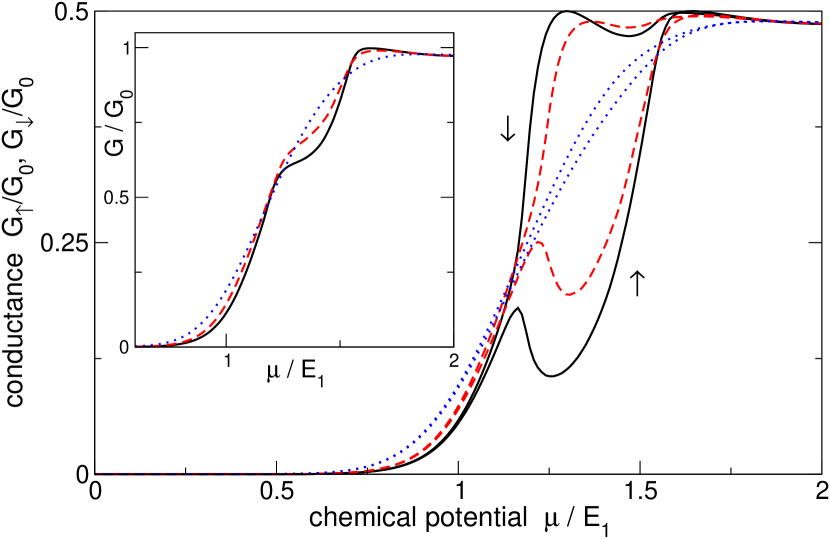
Figure 8: (Color online) The conductance contributions $G_{\uparrow}$ and $G_{\downarrow}$ for $\gamma=4.5\times\hbar^{2}/(2m)$ and for different temperatures $k_{B}T=0$ (solid black line), $k_{B}T=0.029\,E_{1}$ (dashed red line), and $k_{B}T=0.058\,E_{1}$ (dotted blue line). The inset shows the corresponding total conductance $G=G_{\uparrow}+G_{\downarrow}$.

In contrast to our approach the spin-splitting models qualitatively yield the correct temperature dependence Bru01 ; Rei05 . In the model approach, however, the temperature affects only the computation of the conductance whereas the spin-splitting is assumed to be temperature independent. In our calculation the temperature also enters in the computation of the density, Eq. (5), as $G^{<}(E)$ is truncated around the Fermi level plus several $k_{B}T$. Hence, the densities and thus the interaction potentials depend on the temperature which results in a temperature dependent spin-splitting. The spin-gap vanishes at temperatures $k_{B}T\gtrsim 0.08\;E_{1}$. Second, the spin-splitting models assume sharp energy levels with step-like transmission functions $T_{\sigma}(E)=\Theta(E-E_{\sigma})$, where $\Theta(x)$ is the Heaviside step-function. Finite temperatures lead to a smearing of the conductance and a 0.7 structure is found for temperatures smaller than the spin-gap, $k_{B}T<|E_{\uparrow}-E_{\downarrow}|$ Bru01 . In our model the energy levels exhibit a broadening due to the geometry of the system even at zero temperature, $k_{B}T=0$. The broadening is of the order $E_{1}/2$ (see Fig. 2), larger than the level splitting (see Fig. 4). Hence, allowing for finite temperatures the broadening is further enhanced which leads to a decrease of the 0.7 plateau.

IV Discussion and Outlook

IV.1 Electron transport

The presented model describes transport of locally interacting electrons. In Hartree-Fock approximation only electrons with different spins are interacting repulsively. This suggests a very intuitive physical picture: if the scattering region is predominantly occupied by one spin species, electrons with opposite spin are repelled from the constriction. So this kind of interaction favors an asymmetric population of the quantum point contact. Despite its simplicity the model is adequate to qualitatively explain different aspects of the 0.7 anomaly. We see how interaction can cause an asymmetry between the spin-up and spin-down transmission resulting in a shoulder in the total transmission. The magnetic field dependence of the 0.7 feature is well reproduced and we find an instability phenomenon in the zero field case leading to spontaneous spin polarization. Our model also accounts for shot noise suppression at the 0.7 plateau.

Going beyond Hartree-Fock one expects that spin-splitting is weakened or even vanishing in the strict one-dimensional case. However, it was shown by exact methods that Hubbard chain models can have a ferromagnetic ground state if one is not restricted to exactly one-dimensional systems Dau98 ; Kli06 , in accordance with the Lieb-Mattis theorem Lie62 . So in our system which is based on a two-dimensional description a spin polarized ground state is possible.

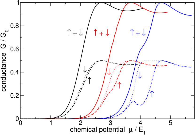
Figure 9: (Color online) Total conductance (solid line) and the up- (dashed) and down (dotted) contributions for different interaction constants $\gamma_{C}$ calculated with full Coulomb interaction. The dimensionless coupling constant takes values $\gamma_{C}=0.18$ (black), $\gamma_{C}=0.20$ (red), and $\gamma_{C}=0.22$ (blue) from left to right. The curves for $\gamma_{C}\geq 0.20$ have been horizontally offset for clarity.

Because the assumption of a delta-like interaction potential might be too crude for the junction in the 2DEG, we also performed calculations with Coulomb interaction and full exchange. For the conductance curves we found similar results as for delta interaction, as shown in Fig. 9 for different coupling strengths. The dimensionless coupling constant can be estimated as

$$\gamma_{C}=\frac{e^{2}}{4\pi\varepsilon_{0}\varepsilon}\frac{2ma^{2}}{\hbar^{2}}\frac{1}{a}\approx 0.20,$$ (12)

where $m=0.07\,m_{0}$, $\varepsilon=13$ and $a=1\,\rm nm$ was inserted. Replacing the Coulomb interaction by a Yukawa potential $V(r)\sim\exp(-r/\lambda)/r$ we find that the results evolve towards the curves for delta interaction with decreasing screening length $\lambda$. So the effect of spin-splitting remains robust even in the limit without screening. In the case of Coulomb interaction the diagonal part of the Fock self-energy also compensates the short-range contribution to the Hartree self-energy, Eq. (3). This leads to an effective short-range repulsion between different spins, similar to the case of delta-interaction. We therefore can conclude that the repulsive interaction between electrons with opposite spin causes spin-splitting even in the case of long-range Coulomb interaction.

Our approach cannot reproduce the experimentally observed temperature dependence of the plateau structure Tho96 , which is also the case for DFT calculations Wan96 ; Ber02 ; Sta03 ; Ber05 . This admits two possible interpretations: On the one hand, Kondo-type correlations could be responsible for the temperature-induced enhancement of the 0.7 feature. This mechanism was theoretically suggested in Ref. Mei02 and experimentally supported in Ref. Cro02 , but still awaits ultimate confirmation by ab initio calculations that are able to take into account such correlations and do not involve any tunable parameter. It was, on the other hand, suggested See03 that phonons could be at the origin of this effect.

IV.2 Transport of fermionic atoms

To discriminate between these two complementary interpretations, we propose to perform transport experiments with ultracold fermionic atoms, such as ⁶Li for instance, which can nowadays be routinely confined within magnetic or optical trapping potentials and cooled down to temperatures close to the BCS transition Zwi05 . In the context of interaction-induced modifications of the conductance, optical (rather than magnetic) techniques for the confinement of the atoms would be required in order to trap both spin species of the fermionic atom. A quasi two-dimensional configuration could, for instance, be realized by a rather strong one-dimensional optical lattice which creates a sequence of disk-like confinement geometries for the atoms, and a matter-wave guide with a constriction could be induced by additional laser beams that are focused onto the disk within which the atoms are confined.

According to Ref. Pet00 , the effective interaction constant $\gamma$ that characterizes the contact potential (2) would, in the case of two-dimensional ultracold fermions, be given by

$$\gamma\simeq\frac{4\pi\hbar^{2}}{m}\frac{1}{\sqrt{2\pi}\frac{a_{\perp}}{a_{s}}+\ln\left(\frac{\hbar\omega_{\perp}}{\pi E}\right)}\,.$$ (13)

Here, $m$ is the mass of the atom, $\omega_{\perp}$ denotes the frequency of the harmonic confinement in the transverse direction (i.e., along the “third” dimension), $a_{\perp}=\sqrt{\hbar/m\omega_{\perp}}$ is the corresponding oscillator length, $E$ denotes the total energy of the collision process between two atoms in the center-of-mass frame, and $a_{s}$ represents the $s$-wave scattering length between two atoms with opposite spin. Both length scales, $a_{s}$ and $a_{\perp}$, can be manipulated, via Feshbach tuning (see, e.g., Ref. Joc03 ) as well as through the intensity of the optical lattice. It would therefore be possible to realize configurations for which the effective interaction strength $\gamma$ is of the order of the values that were discussed in Section III.

To measure the atomic 0.7 anomaly, we propose to prepare the fermionic atoms in a large double-well trap that is optically created within the two-dimensional confinement geometry, and let them escape from one well to the other through a small “bottleneck” corresponding to the constriction of Fig. 1. Counting the number of atoms that are transported across the bottleneck within a finite time scale should give rise to a current of atoms close to the Fermi level. This current can be directly translated into an “atomic conductance” in a similar way as in Ref. Thy99 , which would also display a step-like behavior when the height of the constriction is lowered by optical techniques. Magnetic fields can again be used to break the symmetry between spin-up and spin-down fermions, and the temperature could possibly be controlled by letting the fermionic cloud interact with a gas or condensate of bosonic atoms (e.g., by preparing a mixture of ⁶Li and ⁷Li atoms). As phonons are clearly absent in this setup, any observed feature in the 0.7 anomaly that is not reproducible by mean-field approaches would necessarily be due to (Kondo-type) correlations.

In short summary, is should be possible to realize transport experiments with ultracold fermionic atoms where the 0.7 anomaly in the conductance would be observed. We expect that such experiments would provide new insight into the central mechanism that underlies this phenomenon.

Appendix A Estimation of the model parameters

The coupling constant $\gamma$ is the main parameter of our model. It has to be sufficiently high in order to get an observable effect of the electron-electron interaction. Here we want to estimate an upper limit of the interaction strength using an exponentially screened Coulomb potential.

In a homogeneous 2DEG the screening length $\lambda_{s}$ in Thomas-Fermi approximation is given by And82

$$\lambda_{s}=\frac{2\pi\varepsilon_{0}\varepsilon\hbar^{2}}{me^{2}},$$ (14)

where $\varepsilon$ is the average dielectric constant of the two materials on both sides of the 2DEG. For a GaAs/AlGaAs interface we find $\lambda_{s}\approx 5\,\rm nm$, where $m=0.07\,m_{0}$ and $\varepsilon=13$ was used. To compare the screening length with the width of the constriction, we have to estimate the typical dimensions of a point contact. The lithographic width is of the order of several hundred nanometers, but the electrons are confined by the electrostatic potential due to the gates. The effective width of the constriction is then controlled by the gate voltage. From experiments we know the typical density of carriers $n=1.8\times 10^{11}\,\rm cm^{-2}$ which is related to the chemical potential $\mu=\hbar^{2}\pi n/m$. When the first channel opens the effective width can be estimated by equating the chemical potential with the energy of the first sub-band $\hbar\omega/2$ for a parabolic confinement. The width of the confinement potential at this energy is $W=2\sqrt{\hbar/(m\omega)}$, which gives

$$W=\sqrt{\frac{2}{\pi n}}.$$ (15)

So we find that the effective width of a quantum point contact is of the order $W=20\,\rm nm$. Inside the constriction the density is expected to be lower than in the homogeneous 2DEG, so the effective width will be larger than the above estimated value.

For $\delta$-interaction the coupling constant is given by the spatial integral over the interaction Hamiltonian. So we calculate the corresponding quantity for a screened Coulomb potential

$$\gamma=\frac{e^{2}}{4\pi\varepsilon_{0}\varepsilon}\int{\rm d}^{2}r^{\prime}\frac{{\rm e}^{-|\vec{r}\,^{\prime}|/\lambda_{s}}}{|\vec{r}\,^{\prime}|}=\frac{e^{2}\lambda_{s}}{2\varepsilon_{0}\varepsilon}.$$ (16)

Inserting the screening length, Eq. (14), we find

$$\gamma=2\pi\frac{\hbar^{2}}{2m}.$$ (17)

This is just a rough estimation as several aspects are neglected. First, in Thomas-Fermi approximation the screening length in two dimensions is independent of the electron density. But beyond this approximation one finds an increasing screening length as the charge density goes to zero And82 . This reflects that screening is less efficient if the particle density is too small.

Second, screening in two dimensions is not as strong as in three-dimensional systems. The asymptotic behavior of the screened potential is not exponential, but it follows an $r^{-3}$ law And82 . However, the resulting coupling constant does not differ dramatically from the one obtained by exponential screening. Both facts would give rise to an even higher upper limit of the coupling strength.

Appendix B Recursive algorithm for non-equilibrium Green functions

The recursive Green function algorithm is widely used for calculating electronic properties of two- and three-dimensional systems. The basic idea is to build up the full Green function slice by slice instead of evaluating it in one step. Thus, the dimensions of the matrices that have to be inverted are strongly reduced. If the Green function $G_{0}$ of a semi-infinite region and an adjacent isolated slice is known, it is possible to calculate the Green function $G$ of the coupled system using Dyson’s equation

$$G=G_{0}+G_{0}VG.$$ (18)

(For this derivation we omit the spin index $\sigma$ and the superscript $r$ for the retarded functions). Here, $V$ denotes the hopping matrix between the two adjacent slices. The Green function of a semi-infinite lead can be calculated analytically Fer97 . So it is possible to start with an isolated lead and then add slice by slice until the opposite lead is reached. This is schematically shown in Fig. 10. After coupling that lead to the rest of the system one has obtained the Green function of the complete system at the surface of one lead. This Green function contains all information to calculate the current through the system. The above described procedure is explained for example in Refs. Fer97 ; Mac95 .

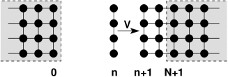
Figure 10: The Green function is constructed by coupling single slices starting from one of the leads (grey regions).

As we are interested also in the electronic density which is determined by the lesser function $G^{<}$, the above explained algorithm is not sufficient. Here we present an extension to the usual recursive Green function method which allows us to calculate the retarded Green function between the two leads as well as the lesser Green function (see also Ref. Lak96 ). The condition to apply this algorithm is that all relevant self-energies are diagonal so that the effective Hamiltonian that has to be inverted, Eq. (6), keeps its block-diagonal structure. This condition is fulfilled for the Hartree self-energy and also for the Fock self-energy in our case of delta interaction. In the general case of full Coulomb interaction the Fock self-energy is not diagonal, see Eq. (3), so the presented method can not be used.

We first show how to add one single slice to a semi-infinite region. In the following we use the notation $G^{S(n)}$ for the Green function of an isolated slice $n$, and $G^{R/L(n)}$ for the Green function of the right/left semi-infinite region starting at slice $n$. The full Green function of the complete (infinite) system is denoted by $G$ (without superscripts). In order to couple the Green function $G^{S(n)}$ of the isolated slice $n$ to the Green function $G^{R(n+1)}$ that covers all lattice sites to the right of $(n+1)$, we use the Dyson equation (18),

$$\left\langle n\left|G^{R(n)}\right|n\right\rangle = \left\langle n\left|\left(G^{S(n)}+G^{R(n+1)}\right)\right|n\right\rangle+$$

$$\left\langle n\left|\left(G^{S(n)}+G^{R(n+1)}\right)VG^{R(n)}\right|n\right\rangle.$$

As $G^{R(n+1)}$ has no matrix elements with slice $n$, the terms $\langle n|G^{R(n+1)}|n\rangle$ vanish and we get

$$\left\langle n\left|G^{R(n)}\right|n\right\rangle = \left\langle n\left|G^{S(n)}\right|n\right\rangle+$$

$$\sum_{a,b}\langle n|G^{S(n)}|a\rangle\langle a|V|b\rangle\langle b|G^{R(n)}|n\rangle.$$

Noting that $G^{S(n)}$ has only non-zero matrix elements with slice $n$ we get the constraint $a=n$. As the coupling matrix $V$ acts only between adjacent slices and has no overlap with other slices $b$ is restricted to the values $n\pm 1$. With $\langle n-1|G^{R(n)}|n-1\rangle=0$ we find

$$G^{R(n)}_{n,n}=G^{S(n)}_{n,n}+G^{S(n)}_{n,n}V_{n,n+1}G^{R(n)}_{n+1,n},$$ (19)

where $G_{n,m}=\langle n|G|m\rangle$ is the sub-matrix of $G$ related to the slices $n$ and $m$. The Green function $G^{R(n)}_{n+1,n}$ appearing in Eq. (19) can be calculated via the Dyson equation in a similar way, and we get

$$G^{R(n)}_{n+1,n}=G^{R(n+1)}_{n+1,n+1}V_{n+1,n}G^{R(n)}_{n,n}.$$

Inserting this result into Eq. (19) and solving for $G^{R(n)}_{n,n}$ we obtain

$$G^{R(n)}_{n,n}=\left[(E-H_{n,n})-V_{n,n+1}G^{R(n+1)}_{n+1,n+1}V_{n+1,n}\right]^{-1},$$ (20)

where we used $G^{S(n)}_{n,n}=(E-H_{n,n})^{-1}$. Therefore, Eq. (20) allows us to calculate the Green function covering all lattice sites to the right of slice $n$ from the Green function to the right of $(n+1)$. In that way we have added one slice. Iterating this scheme we can finally obtain the Green function $G^{R(1)}_{1,1}$ at the left end of the scattering region. Then one has to connect the Green functions of the two semi-infinite sections to get the full Green function $G_{1,1}$ (without superscript) at the left end of the scatterer. This we obtain by using the Dyson equation

$$\left\langle 1\left|G\right|1\right\rangle = \left\langle 1\left|\left(G^{L(0)}+G^{R(1)}\right)\right|1\right\rangle+$$

$$\left\langle 1\left|\left(G^{L(0)}+G^{R(1)}\right)VG\right|1\right\rangle,$$

and we find

$$G_{1,1}=\left[1-G^{R(1)}_{1,1}V_{1,0}G^{L(0)}_{0,0}V_{0,1}\right]^{-1}G^{R(1)}_{1,1}.$$ (21)

In this equation $G^{L(0)}_{0,0}$ is the surface Green function of the semi-infinite left lead. The Green function $G_{1,1}$ contains all information about the reflection coefficients at the left lead.

In an analog way we can start from the left lead and calculate all Green functions from left to right by

$$G^{L(n)}_{n,n}=\left[(E-H_{n,n})-V_{n,n-1}G^{L(n-1)}_{n-1,n-1}V_{n-1,n}\right]^{-1},$$ (22)

and finally obtain the full Green function at the right end of the scatterer,

$$G_{N,N}=\left[1-G^{L(N)}_{N,N}V_{N,N+1}G^{R(N+1)}_{N+1,N+1}V_{N+1,N}\right]^{-1}G^{L(N)}_{N,N}.$$ (23)

Here $G^{R(N+1)}_{N+1,N+1}$ is the surface Green function of the right lead.

Knowing the full Green functions at both ends of the scatterer, $G_{1,1}$ and $G_{N,N}$, we can now compute the full Green functions between the ends and any slice $n$ inside the scattering region. We use the Dyson equation

$$\left\langle n\left|G\right|1\right\rangle = \left\langle n\left|\left(G^{L(n-1)}+G^{R(n)}\right)\right|1\right\rangle+$$

$$\left\langle n\left|\left(G^{L(n-1)}+G^{R(n)}\right)VG\right|1\right\rangle$$

to obtain

$$G_{n,1}=G^{R(n)}_{n,n}V_{n,n-1}G_{n-1,1},$$ (24)

where the $G^{R(n)}_{n,n}$ are calculated from Eq. (20). Analogously one finds

$$G_{n,N}=G^{L(n)}_{n,n}V_{n,n+1}G_{n+1,N}$$ (25)

with the Green functions $G^{L(n)}_{n,n}$ from Eq. (22). The last two equations allow us to compute the Green functions $G_{n,1}$ and $G_{n,N}$ recursively by starting with the Green functions $G_{1,1}$ and $G_{N,N}$ at the ends of the scattering region.

Now it is possible to compute the diagonal elements of the lesser Green function which are needed to calculate the electron density, Eq. (5). A diagonal matrix element of $G^{<}$ reads according to Eq. (7)

$$\left[G^{<}\right]_{xx}=\sum_{i,j}[G]_{xi}\left[\Sigma^{<}\right]_{ij}[G]_{xj}^{*}$$ (26)

with $i,j\in\{n=1,n=N\}$. The self-energy $\Sigma^{<}$ is only non-zero at the ends of the scatterer where the lattice sites are coupled to the leads. So the indices $i$ and $j$ are from the first and last slice of the scattering region. Therefore, the Green functions calculated from Eqs. (24) and (25) enter here.

The complete recursive procedure can be summarized in the following steps:

• calculate and store all $G^{R(n)}_{n,n}$ from the lead Green function $G^{R(N+1)}_{N+1,N+1}$ by means of Eq. (20);

• calculate and store all $G^{L(n)}_{n,n}$ from the lead Green function $G^{L(0)}_{0,0}$ by means of Eq. (22);

• compute the full Green functions $G_{1,1}$ and $G_{N,N}$ at the left and right end of the scatterer using Eqs. (21) and (23);

• use Eqs. (24) and (25) to calculate and store all $G_{n,1}$ and $G_{n,N}$ from $G_{1,1}$ and $G_{N,N}$. One of those Green functions is $G_{N,1}$ which contains information about the transport properties;

• finally, one obtains the diagonal elements of $G^{<}$ from $G_{n,1}$ and $G_{n,N}$ by means of Eq. (26).
  

In total, one has to run four times through the entire system in order to be able to calculate $G^{<}$ as well as parts of $G^{r}$ which are needed for the reflection and transmission coefficients. If the calculation of $G^{<}$ is not necessary it is enough to pass the system twice to get all reflection and transmission coefficients. So the scheme reduces to the standard recursive algorithm Fer97 ; Mac95 . If one is only interested in the current, passing the scatterer once is sufficient. After computing $G_{1,1}$ with Eq. (21) the total reflection is known. Employing current conservation (unitarity) it is possible to get the total transmission and hence the current.

References

- (1) B. J. van Wees, H. van Houten, C. W. J. Beenakker, J. G. Williamson, L. P. Kouwenhoven, D. van der Marel, and C. T. Foxon, Phys. Rev. Lett. 60, 848 (1988)
- (2) D. A. Wharam, T. J. Thornton, R. Newbury, M. Pepper, H. Ahmed, J. E. F. Frost, D. G. Hasko, D. C. Peacock, D. A. Ritchie, and G. A. C. Jones, J. Phys. C 21, L209 (1988)
- (3) A. Khurana, Physics Today November 1988, p21 (1988)
- (4) for an overview see e.g. C. W. J. Beenakker, and H. van Houten, Sol. State Phys. 44, 1 (1991); cond-mat/0412664
- (5) K. J. Thomas, J. T. Nicholls, M. Y. Simmons, M. Pepper, D. R. Mace, D. A. Ritchie, Phys. Rev. Lett. 77, 135 (1996)
- (6) K. J. Thomas, J. T. Nicholls, N. J. Appleyard, M. Y. Simmons, M. Pepper, D. R. Mace, W. R. Tribe, and D. A. Ritchie, Phys. Rev. B 58, 4846 (1998)
- (7) A. Kristensen, H. Bruus, A. E. Hansen, J. B. Jensen, P. E. Lindelof, C. J. Marckmann, J. Nygård, C. B. Sørensen, F. Beuscher, A. Forchel, and M. Michel, Phys. Rev. B 62, 10950 (2000)
- (8) S. Nuttinck, K. Hashimoto, S. Miyashita, T. Saku, Y. Yamamoto, and Y. Hirayama, Jpn. J. Appl. Phys. 39, L655 (2000)
- (9) D. J. Reilly, G. R. Facer, A. S. Dzurak, B. E. Kane, R. G. Clark, P. J. Stiles, R. G. Clark, A. R. Hamilton, J. L. O’Brien, N. E. Lumpkin, L. N. Pfeiffer, and K. W. West, Phys. Rev. B 63, 121311(R) (2001)
- (10) S. M. Cronenwett, H. J. Lynch, D. Goldhaber-Gordon, L. P. Kouwenhoven, C. M. Marcus, K. Hirose, N. S. Wingreen, and V. Umansky, Phys. Rev. Lett. 88, 226805 (2002)
- (11) D. J. Reilly, T. M. Buehler, J. L. O’Brien, A. R. Hamilton, A. S. Dzurak, R. G. Clark, B. E. Kane, L. N. Pfeiffer, and K. W. West, Phys. Rev. Lett. 89, 246801 (2002)
- (12) L. P. Rokhinson, L. N. Pfeiffer, and K. W. West, Phys. Rev. Lett. 96, 156602 (2006)
- (13) P. Roche, J. Ségala, D. C. Glattli, J. T. Nicholls, M. Pepper, A. C. Graham, K. J. Thomas, M. Y. Simmons, and D. A. Ritchie, Phys. Rev. Lett. 93, 116602 (2004)
- (14) L. DiCarlo, Y. Zhang, D. T. McClure, D. J. Reilly, C. M. Marcus, L. N. Pfeiffer, and K. W. West, Phys. Rev. Lett. 97, 036810 (2006)
- (15) for a short recent review see K.-F. Berggren, Turk. J. Phys. 30, 197 (2006)
- (16) C.-K. Wang and K.-F. Berggren, Phys. Rev. B 54, R14257 (1996)
- (17) K.-F. Berggren and I. I. Yakimenko, Phys. Rev. B 66, 085323 (2002)
- (18) A. A. Starikov, I. I. Yakimenko, and K.-F. Berggren, Phys. Rev. B 67, 235319 (2003)
- (19) K.-F. Berggren, P. Jaksch, and I. Yakimenko, Phys. Rev. B 71, 115303 (2005)
- (20) H. Bruus, V. V. Cheianov, and K. Flensberg, Physica E 10, 97 (2001)
- (21) D. J. Reilly, Phys. Rev. B 72, 033309 (2005)
- (22) D. J. Reilly, Y. Zhang, and L. DiCarlo, Physica E 34, 27 (2006)
- (23) Y. Meir, K. Hirose, and N. S. Wingreen, Phys. Rev. Lett. 89, 196802 (2002)
- (24) K. Hirose, Y. Meir, and N. S. Wingreen, Phys. Rev. Lett. 90, 026804 (2003)
- (25) G. Seelig and K. A. Matveev, Phys. Rev. Lett. 90, 176804 (2003)
- (26) A. Golub, T. Aono, and Y. Meir, cond-mat/0605114 (2006)
- (27) T. Rejec and Y. Meir, Nature 442, 900 (2006)
- (28) S. Datta: Electronic Transport in Mesoscopic Systems (Cambridge University Press, 1995)
- (29) J. Rammer and H. Smith, Rev. Mod. Phys. 58, 323 (1986)
- (30) see for example: D. Frustaglia, M. Hentschel, and K. Richter, Phys. Rev. B 69, 155327 (2004)
- (31) D. K. Ferry and S. M. Goodnick: Transport in Nanostructures (Cambridge University Press, 1997)
- (32) Ya. M. Blanter and M. Büttiker, Phys. Rep. 336, 1 (2000)
- (33) S. Daul and R. M. Noack, Phys. Rev. B 58, 2635 (1998)
- (34) A. D. Klironomos, J. S. Meyer, and K. A. Matveev, Europhys. Lett. 74, 679 (2006)
- (35) E. Lieb and D. Mattis, Phys. Rev. 125, 164 (1962)
- (36) M. W. Zwierlein, J. R. Abo-Shaeer, A. Schirotzek, C. H. Schunck, and W. Ketterle, Nature 435, 1047 (2005).
- (37) D. S. Petrov, M. Holzmann, and G. V. Shlyapnikov, Phys. Rev. Lett. 84, 2551 (2000).
- (38) S. Jochim, M. Bartenstein, A. Altmeyer, G. Hendl, S. Riedl, C. Chin, J. Hecker Denschlag, and R. Grimm, Science 302, 2101 (2003).
- (39) J. H. Thywissen, R. M. Westervelt, and M. Prentiss, Phys. Rev. Lett. 83, 3762 (1999).
- (40) T. Ando, A. B. Fowler, and F. Stern, Rev. Mod. Phys. 54, 437 (1982); Note: the authors are using cgs-units.
- (41) M. Macucci, A. Galick, and U. Ravaioli, Phys. Rev. B 52, 5210 (1995)
- (42) R. Lake, G. Klimeck, R. C. Bowen, and D. Jovanovic, J. Appl. Phys. 81, 7845 (1996)